Bayesian Network Constraint-Based Structure Learning Algorithms: Parallel and Optimised Implementations in the bnlearn R Package

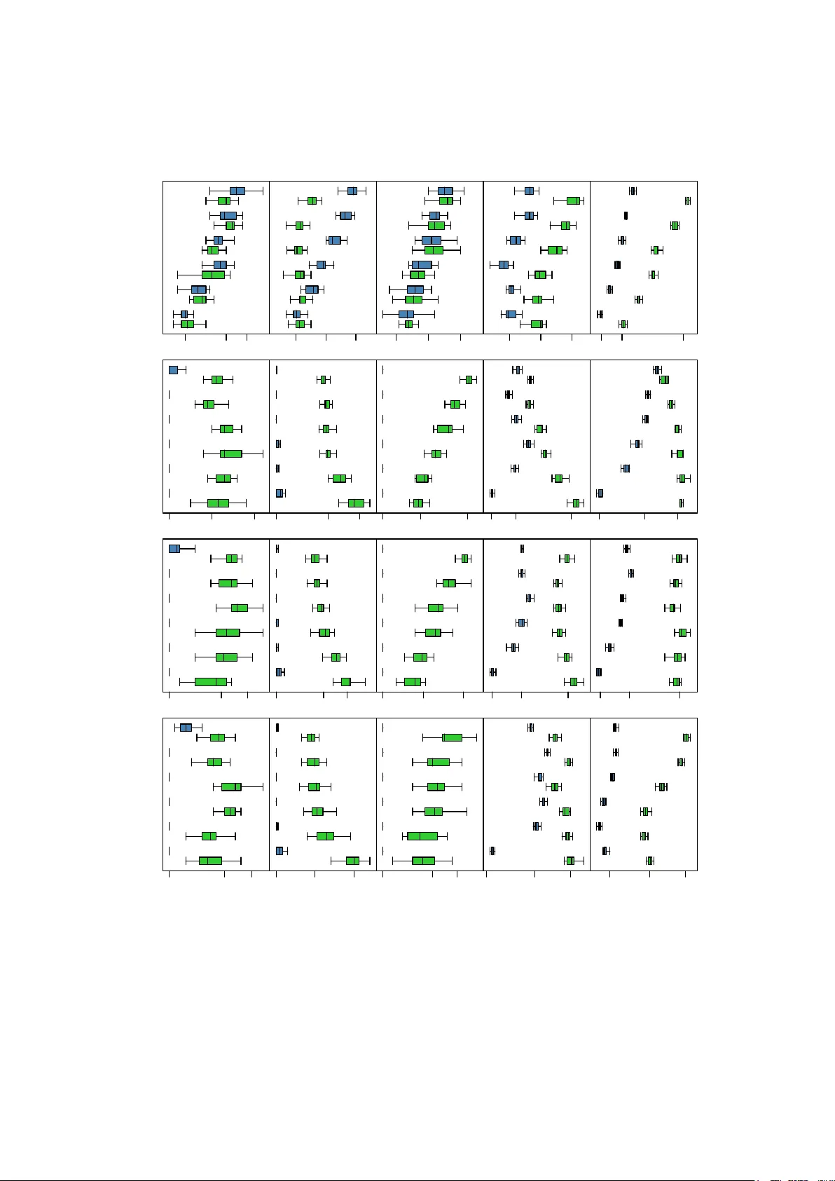
J S S Journal of Statistical Software MMMMMM YYYY, V olume VV, Issue II. http://www.jstatsoft.or g/ Ba y esian Net w ork Constrain t-Based Structure Learning Algorithms: P arallel and Optimised Implemen tations in the bnlearn R P ac k age Marco Scutari Univ ersit y of Oxford Abstract It is w ell known in the l iterature that the problem of l earning the structure of Ba y esian net works is v ery hard to tac kle: its computational complexit y is sup er-exponential in the n umber of nodes in the worst case and p olynomial in most real-world scenarios. Efficien t implemen tations of score-based structure learning b enefit from past and cur- ren t researc h in optimisation theory , which can b e adapted to the task b y using the net- w ork score as the ob jective function to maximise. This is not true for approaches based on conditional indep endence tests, called constrain t-based learning algorithms. The only optimisation in widespread use, backtrac king, leverages the symmetries implied by the definitions of neighbourho od and Marko v blank et. In this paper we illustrate how backtrac king is implemented in recent versions of the bnlearn R pack age, and how it degrades the stabilit y of Bay esian netw ork structure learn- ing for little gain in terms of sp eed. As an alternative, we describe a softw are architecture and framework that can b e used to parallelise constraint-based structure learning algo- rithms (also implemen ted in bnlearn ) and we demonstrate its p erformance using four reference netw orks and t wo real-world data sets from genetics and systems biology . W e sho w that on mo dern multi-core or multiprocessor hardw are parallel implementations are preferable ov er backtrac king, whic h w as dev elop ed when single-processor mac hines w ere the norm. Keywor ds : Bay esian net works, structure learning, parallel programming, R . 1. Bac kground and notations Ba yesian net w orks (BNs) are a class of gr aphic al mo dels ( P earl 1988 ; Koller and F riedman 2009 ) comp osed by a set of random v ariables X = { X i , i = 1 , . . . , m } and a dir e cte d acyclic gr aph (D AG), denoted G = ( V , A ) where V is the no de set and A is the ar c set . The 2 Ba yesian Netw ork Learning: P arallel and Optimised Implemen tations probabilit y distribution of X is called the glob al distribution of the data, while those associated with individual X i s are called lo c al distributions . Eac h no de in V is asso ciated with one v ariable, and they are referred to in terc hangeably . The directed arcs in A that connect them are denoted as “ → ” and represen t direct sto c hastic dep endencies; so if there is no arc connecting tw o no des, the corresponding v ariables are either marginally indep enden t or conditionally indep enden t given (a subset of ) the rest. As a result, eac h lo cal distribution dep ends only on a single no de X i and on its paren ts (i.e., the nodes X j , j 6 = i such that X j → X i , here denoted Π X i ): P ( X ) = m Y i =1 P ( X i | Π X i ) . (1) Common choices for the lo cal and global distributions are multinomial v ariables (discrete BNs, Heck erman, Geiger, and Chick ering 1995 ); univ ariate and multiv ariate normal v ariables (Gaussian BNs, Geiger and Hec k erman 1994 ); and, less frequently , a com bination of the t w o (conditional Gaussian (CG) BNs, Laurit zen and W ermuth 1989 ). In the first case, the param- eters of interest are the conditional probabilities asso ciated with each v ariable, represen ted as c onditional pr ob ability tables (CPTs); in the second, the parameters of intere st are the p artial c orr elation c o efficients b et w een eac h v ariable and its paren ts. As for CG BNs, the parameters of interest are again partial correlation co efficien ts, computed for each no de conditional on its contin uous paren ts for each configuration of the discrete paren ts. The key adv an tage of the decomposition in Equation ( 1 ) is to mak e lo c al c omputations p ossible for most tasks, using just a few v ariables at a time regardless of the magnitude of m . A relat ed quan tit y that works to the same effect is the Markov blanket of each no de X i , defined as the set B ( X i ) of nodes which graphicall y separates X i from all other nodes V \ { X i , B ( X i ) } ( Pearl 1988 , p. 97). In BNs such a set is uniquely ident ified by the paren ts ( Π X i ), the children (i.e., the no des X j , j 6 = i suc h that X i → X j ) and the sp ouses of X i (i.e., the nodes that share a c hild with X i ). By definition, X i is indep enden t of all other no des given B ( X i ), th us making them redundant for inference on X i . The task of fitting a BN is called le arning and is generally implemen ted in tw o steps. The first is called structur e le arning , and consists in finding the D AG that enco des the con- ditional indep endencies present in the data. This has b een ac hiev ed in the literature with c onstr aint-b ase d , sc or e-b ase d and hybrid algorithms; for an ov erview see Koller and F riedman ( 2009 ) and Scutari and Denis ( 2014 ). Constraint -based algorithms are based on the seminal w ork of Pearl on causal graphical mo dels and his Inductive Causation algorithm (IC, V erma and P earl 1991 ), whi ch provides a framework for learning the D AG of a BN using condi- tional indep endence tests under the assumption that graphical separation and probabilistic indep endence imply each other (the faithfulness assumption). T ests in common use are the m utual information test (for discrete BNs) and the exact Studen t’s t test for correlation (for GBNs). Score-based algorithms represen t an application of heuristic optimisation techniques: eac h candidate D AG is assigned a netw ork score reflecting its go odness of fit, whic h the algo- rithm then attempts to maximise. BIC and p osterior probabilities arising from v arious priors are t ypical c hoices. Hybrid algorithms use b oth conditional indep endence tests and netw ork scores, the former to reduce the space of candidate DA Gs and the latter to iden tify the op- timal DA G among them. Some examples are PC (named after its in v entors Peter Spirtes and Clark Glymour; Spirtes, Glymour, and Sc heines 2000 ), Gro w-Shrink (GS; Margaritis Journal of Statistical Softw are 3 2003 ), Incremental Asso ciation (IAMB; Tsamardinos, Alif eris, and Statnik ov 2003 ), In ter- lea ved IAMB (In ter-IAMB; Y aramak ala and Margaritis 2005 ), hill-clim bing and tabu search ( Russell and Norvig 2009 ), Max-Min Paren ts & Children (MMPC; Tsamardinos, Bro wn, and Aliferis 2006 ) and the Semi-In terlea ved HITON-PC (SI-HITON-PC, from the Greek “hiton” for “blank et” ; Aliferis, Statnik ov, Tsamardinos, Mani, and Xenofon 2010 ). These algorithms and more are implemented across several R pac k ages, such as bnlearn (all of the ab o v e except PC; Scutari 2010 ), deal (hill-climbing; Bøttcher and Dethlefsen 2003 ), catnet and m ugnet (sim ulated annealing; Balov and Salzman 2013 ; Balov 2013 ), p calg (PC and causal graphical mo del learning algorithms; Kalisc h, M ¨ ac hler, Colom b o, Maath uis, and B ¨ uhlmann 2012 ) and abn (hill clim bing and exact algorithms; Lewis 2013 ). F urther extensions to model dynamic data are implemen ted in eb dbNet ( Rau, Jaffr´ ezic, F oulley , and Do erge 2010 ), G1DBN ( L` ebre 2013 ) and AR TIV A ( L ` ebre, Becq, Dev aux, Lelandais, and Stumpf 2010 ) among others. The second step is called p ar ameter le arning and, as the name suggests, deals with the esti- mation of the parameters of the global distribution. Since the graph structure is known from the previous step, this can b e done efficiently by estimating the parameters of the lo cal dis- tributions. With the exception of bnlearn , which has a separate bn.fit function, R pack ages automatically execute this step along with structure learning. Most problems in BN theory ha ve a computational complexit y that, in the worst case, scales exp onen tially with the num b er of v ariables. F or instance, b oth structure learning ( Chic ker- ing 1996 ; Chic kerin g, Geiger, and Heck erman 1994 ) and inference ( Co op er 1990 ; Dagum and Lub y 1993 ) are NP-hard and hav e p olynomial complexit y ev en for sparse netw orks. This is esp ecially problematic in high-dimensional settings such as genetics and systems biology , in whic h BNs are used for the analysis of gene expressions ( F riedman 2004 ) and protein-protein in teractions ( Jansen, Y u, Green baum, Kluger, Krogan, Ch ung, Emi li, Sn yder, Greenblatt, and Gerstein 2003 ; Sac hs, P erez, P e’er, Lauffen burger, and Nolan 2005 ); for in tegrating het- erogeneous ge netic data ( Chang and M cGeachie 2011 ); and to determine disease susceptibilit y to anemia ( Sebastiani, Ramoni, Nolan, Baldwin, and Steinberg 2005 ) and hypertension ( Mal- o vini, Nuzzo, F errazzi, Puca, and Bellazzi 2009 ). Ev en though algorithms in recen t literature are designed taking scalability in to accoun t, it is often impractical to learn BNs from data containing more than few hundr eds of v ariables without restrictive assumptions on either the structure of the DA G or the nature of the lo cal distributions. Tw o wa ys to address this problem are: 1. optimisations: reducing the num ber of conditional indep endence tests and netw ork scores computed from the data, either b y skipping redundant ones or b y limiting local computations to a few v ariables; 2. p ar al lel implementations: splitting learning across m ultiple cores and processors to mak e b etter use of mo dern mu lti-core and m ultipro cessor hardware. As far as score-based learning algorithms are concerned, b oth p ossibilities ha v e b een explored and a wide range of solutions prop osed, from efficien t cac hing using decomposable scores ( Daly and Shen 2007 ), to parallel meta-heuristics ( Raub er and R ¨ unger 2010 ) and in teger programming ( Cussens 2011 ). The same cannot b e said of constrain t-based algorithms; ev en recen t ones suc h as SI-HITON-PC, while efficient , are still implemented with basic bac ktrac k- ing as the only optimisation. W e will examine them and their implementations in Section 2 , arguing that bac ktrac king pro vides only mo dest sp eed gains and increases the v ariability of 4 Ba yesian Netw ork Learning: P arallel and Optimised Implemen tations the learned DA Gs. As an alternative, in Section 3 we describe a softw are archi tecture and framew ork that can b e used to create parallel i mplementations of con straint-based al gorithms that scale well on large data sets and do not suffer from this problem. In b oth sections we will fo cus on the bnlearn pack age b ecause it provides the widest choice of algorithms and implemen tations among those of interest for this pap er. 2. Constrain t-based structure learning and bac ktrac king All constraint-bas ed structure learning algorithms share a common three-phase structure in- herited from the IC algorithm through PC and GS; it is illustrated in Algorithm 1 . The first, optional, phase consists in learning the Marko v blanket of each no de to reduce the num b er of candidate D AGs early on. An y algorithm for learning Marko v blankets can b e plugged in step 1 and extended into a full BN structure learning algorithm, as originally suggested in Margaritis ( 2003 ) for GS. Once all Mark o v blank ets hav e b een learned, they are chec ked for consistency (step 2 ) using their symmetry; b y definition X i ∈ B ( X j ) ⇔ X j ∈ B ( X i ). Asym- metries are corrected by treating them as false p ositiv es and removing the offending no des from each other’s Mark o v blankets. The second phase learns the skeleton of the DA G, that is, it identifies whic h arcs are presen t in the D AG mo dulo their direction. This is equiv alen t to learning the neighb ours N ( X i ) of eac h no de: its paren ts and children . As illustrated in step 3 , the absence of a set of no des S X i X j that separates a particular pair X i , X j implies that either X i → X j or X j → X i . Separating sets are considered in order of increasing size to k eep computations as lo cal as p ossible. F urthermore, if B ( X i ) and B ( X j ) are a v ailable from steps 1 and 2 the searc h space can be greatly reduced b ecause N ( X i ) ⊆ B ( X i ). On the one hand, if X j / ∈ B ( X i ) b y definition X i is separated from X j b y S X i X j = B ( X i ). On the other hand, if X j ∈ B ( X i ) most candidate sets can b e disregarded b ecause we kno w that S X i X j ⊆ B ( X i ) \ X j and S X i X j ⊆ B ( X j ) \ X i ; b oth sets are t ypically muc h smaller than V . With the exception of the PC algorithm, whic h is structured exactly as describ ed in step 3 , constraint-based algorithms learn the skeleton b y learning each N ( X i ) and then enforcing symmetry (step 4 ). Finally , in the third phase arc directions are established as in Meek ( 1995 ). It is imp ortan t to note that, for some arcs, b oth directions are equiv alent in the sense that they identify equiv- alen t decomp ositions of the global distribution. Therefore, some arcs will be left undirected and the algorithm will return a c omplete d p artial ly dir e cte d acyclic gr aph identifying an e quiv- alenc e class containing multipl e DA Gs. Suc h a class is uniquely identified by the skeleton learned in steps 3 and 4 , and by the v-structur es V l of the form X i → X k ← X j , X i / ∈ N ( X j ) learned in step 5 ( Chick ering 1995 ). Additional arc directions are inferred indirectly in step 6 b y ruling out those that w ould in tro duce additional v-structures (which would hav e been iden tified in step 5 ) or cycles (whic h are not allo wed in D A Gs). Ev en in such a general form, we can see that Algorithm 1 p erforms many c hecks for graphical separation that are redundan t giv en the symmetry of the B ( X i ) and the N ( X i ). In tuitiv ely , once w e ha v e concluded that X j / ∈ B ( X i ) there is no need to chec k whether X i ∈ B ( X j ) in step 1 ; and similar considerations can b e made for neigh b ours in step 3 . In practice, this translates to redundant indep endence tests computed on the data. Therefore, up to version 3.4 bnlearn implemen ted b acktr acking b y assuming X 1 , . . . , X m w ere pro cessed sequen tially and enforcing symmetry by construction (e.g., if i < j then X j / ∈ B ( X i ) ⇒ X i / ∈ B ( X j ) and Journal of Statistical Softw are 5 Algorithm 1 A template for constrain t-based structure learning algorithms Input: a data set con taining the v ariables X i , i = 1 , . . . , m . Output: a completed partially directed acyclic graph. Phase 1: learning Marko v blankets (optional). 1. F or each v ariable X i , learn its Mark o v blanket B ( X i ). 2. Check whether the Marko v blankets B ( X i ) are symmetric, e.g., X i ∈ B ( X j ) ⇔ X j ∈ B ( X i ). Assume that no des for whom symmetry do es not hold are false p ositiv es and drop them from eac h other’s Marko v blankets . Phase 2: learning neighbours. 3. F or each v ariable X i , learn the set N ( X i ) of its neigh b ours (i.e., the parents and the c hildren of X i ). Equiv alen tly , for each pair X i , X j , i 6 = j searc h for a set S X i X j ⊂ V (including S X i X j = ∅ ) such that X i and X j are indep enden t giv en S X i X j and X i , X j / ∈ S X i X j . If there is no suc h a set, place an undirected arc b et ween X i and X j ( X i − X j ). If B ( X i ) and B ( X j ) are av ailable from p oin ts 1 and 2 , the search for S X i X j can b e limited to the smallest of B ( X i ) \ X j and B ( X j ) \ X i . 4. Check whether the N ( X i ) are symmetric, and correct asymmetries as in step 2 . Phase 3: learning arc directions. 5. F or each pair of non-adjacen t v ariables X i and X j with a common neighbour X k , chec k whether X k ∈ S X i X j . If not, set the direction of the arcs X i − X k and X k − X j to X i → X k and X k ← X j to obtain a v-structure V l = { X i → X k ← X j } . 6. Set the direction of arcs that are still undirected b y applying the follo wing t wo rules recursiv ely: (a) If X i is adjacent to X j and there is a strictly directed path from X i to X j (a path leading from X i to X j con taining no undirected arcs) the n set th e direction of X i − X j to X i → X j . (b) If X i and X j are not adjacen t but X i → X k and X k − X j , then change the latter to X k → X j . X j ∈ B ( X i ) ⇒ X i ∈ B ( X j )). While this app roach on av erage reduces the n um b er of tests by a factor of 2, it also in tro duces a false p ositiv e or a false negativ e in the learning pro cess for ev ery t yp e I or type I I error in the independence tests. As long as BN learning was only feasible for simple data sets (due to limitations in computational pow er and algorithm efficiency), and the fo cus w as on probabilistic mo delling, the ov erall error rate w as still acceptable; but the increasing prev alence of causal mo delling on “small n , large p ” data sets in many fields requires a b etter approac h. One such is described in Tsamardinos et al. ( 2006 , p. 46) and implemen ted in bnlearn from versi on 3.5. It mo difies steps 1 and 3 as follows: • If X j / ∈ B ( X i ) , i < j , then do not consider X i for inclusion in B ( X j ); and if X j / ∈ N ( X i ), 6 Ba yesian Netw ork Learning: P arallel and Optimised Implemen tations then do not consider X i for inclusion in N ( X i ). • If X j ∈ B ( X i ) , then consider X i for inclusion in B ( X j ) by initialising B ( X j ) = { X i } ; and if X j ∈ N ( X i ) then initialise N ( X j ) = { X i } . Note that in b oth cases X i can be discarded in the process of learning B ( X j ) and N ( X j ). Ev en in this form, bac ktrac king has the undesirable effect of mak ing structure learning depend on the order the v ariables are stored in the data set, whic h has b een shown to increase errors in the PC algorithm ( Colombo and Maathuis 2013 ). In addition, bac ktrac king provides only a mo dest sp eed increase compared to a parallel implementation of steps 1 - 4 ; w e will compare the resp ectiv e running times in Section 3 . How ever, it is easy to implement side-by-side with the original versions of constrain t-based structure learning algorithms. Such algorithms are t ypically describ ed only at the no de level, that is, they define how each B ( X i ) and N ( X i ) is learned and then they combine them as describ ed in Algorithm 1 . bnlearn exp orts t wo functions that giv e access to the corresponding back ends: learn.mb to learn a single B ( X i ) and learn.nbr to learn a single N ( X i ). The old approac h to backtrac king essentially whitelisted all no des suc h that X j ∈ B ( X i ) and blacklisted all no des suc h that X j / ∈ B ( X i ) for each X i . R> library(bnlearn) R> data(learning.test) R> learn.nbr(x = learning.test, method = "si.hiton.p c", node = "D", + whitelist = c("A", "C"), blacklist = "B") F or example, in the co de ab o v e we learn N ( D ) and, assuming we already learned N ( A ), N ( B ) and N ( C ), we whitelist and blacklist A , B and C dep ending on whether D was one of their neigh b ours or not. The remaining no des in the BN are neither whitelisted nor blacklisted and are then tested for conditional indep endence. By con trast, the current approach initialises N ( D ) as { A , C } but do es not whitelist those no des. R> learn.nbr(x = learning.test, method = "si.hiton.p c", node = "D", + blacklist = "B", start = c("A", "C")) As a result, both A and C can b e remo ved from N ( D ) by the algorithm. The v anilla, non- optimised equiv alent for the same learning algorithm w ould b e R> learn.nbr(x = learning.test, method = "si.hiton.p c", node = "D") whic h do es not include an y information from N ( A ), N ( B ) or N ( C ). The syn tax for learn.mb is identical, and will b e omitted for brevit y . The only other R pac k age implemen ting general constrain t-based structure learning, p calg , implemen ts the PC algorithm as a monolithic function and do es not export the back ends whic h are used to learn the presence of an arc b et w een a pair of nodes. F urthermore, as we noted abov e, PC is implemen ted differen tly from other constrain t-based algorithms and is usually mo dified with different optimisations than bac ktrac king; see, for instance, the interlea ving describ ed in Colombo and Maath uis ( 2013 ). In the remainder of this section we will fo cus on the effects of bac ktracking on learning the sk eleton of the DA G, b ecause steps 1 - 4 comprise the v ast ma jority of the o ver all conditional indep endence tests and thus control most of the v ariabilit y of the DA G. T o inv estigate it, we used bnlearn and 5 reference BNs of v arious size and complexit y from http://www.bnlearn. com/bnrepository : Journal of Statistical Softw are 7 • ALARM ( Beinlic h, Suermondt, Chav ez, and Co op er 1989 ), with 37 no des, 46 arcs and p = 509 parameters. A BN designed b y medical exp erts to provid e an alarm message system for in tensive care unit patie nts based on th e outpu t a n um b er of vital signs monitoring devices. • HEP AR I I ( Onisko 2003 ), with 70 nodes, 123 arcs and p = 1453 parameters. A BN mo del for the diagnosis of liv er disorders from related clinical conditions (e.g., gallstones) and relev ant biomark ers (e.g., bilirubin, hepatocellular mark ers). • ANDES ( Conati, Gertner, V anLehn, and Druzdzel 1997 ), with 223 no des, 338 arcs and p = 1157 parameters. An intelligen t tutoring system based on a studen t mo del for the field of classical Newtonian ph ysics, dev elop ed at the Univ ersity of Pittsburgh and at the United States Nav al Academy . It handles long-term kno wledge assessment, plan recognition, and prediction of studen ts’ actions during problem solving exercises. • LINK ( Jensen and Kong 1999 ), with 724 no des, 1125 arcs and p = 14211 parameters. Dev elop ed in the context of link age analysis in large p edigrees, it mo dels the link age and the distance betw een a causal gene and a genetic mark er. • MUNIN ( Andreassen, Jensen, Andersen, F alck, Kjærulff, W oldb y e, Sørensen, Rosen- falc k, and Jensen. 1989 ), with 1041 no des, 1397 arcs with p = 80592 parameters. A BN designed b y exp erts to in terpret results from electromy ographic examinations and diagnose a large set of common diseases from ph ysical conditions such as atroph y and activ e nerve fibres. Sim ulations w ere performed on a cluster of 7 dual AMD Opt eron 6136, eac h with 16 cores and 78GB of RAM, with R 3.1.0 and bnlearn 3.5. F or each BN, w e considered 6 different sample sizes ( n = 0 . 1 p, 0 . 2 p, 0 . 5 p, p, 2 p, 5 p ), chosen as m ultiples of p to facilitate comparisons b et w een net work s of suc h differen t complexit y; and 4 different constrain t-based structure learning algorithms (GS, In ter-IAMB, MMPC, SI-HITON-PC). Since all reference BNs are discrete, w e used the asymptotic χ 2 m utual information test with α = 0 . 01. F or eac h combination of BN, sample size and algorithm we repeated the follo wing simulation 20 times. First, we loaded the BN from the RDA file do wnloaded from the rep ository ( alarm.rda b elo w) and generated a sample of the appropriate size with rbn . R> load("alarm.rda") R> sim = rbn(bn, n = round(0.1 * nparams(bn))) F rom that sample, w e learned the sk eleton of the D A G wit h ( optimiz ed = TRUE ) and without bac ktrac king ( optimized = FALSE ). R> skel.orig = skeleton(si.hiton.pc(sim, test = "mi", alpha = 0.01, + optimized = FALSE)) R> skel.back = skeleton(si.hiton.pc(sim, test = "mi", alpha = 0.01, + optimized = TRUE)) Subsequen tly , we rev ersed the order of the columns in the data to inv estigate whether this results in a differen t skeleton. 8 Ba yesian Netw ork Learning: P arallel and Optimised Implemen tations Hamming distance n/p ALARM ANDES HEP AR II LINK MUNIN SI−HIT ON−PC MMPC Inter−IAMB GS 0.1 0.2 0.5 1.0 2.0 5.0 0 10 15 0 20 40 0 10 15 0 120 210 150 250 340 0.1 0.2 0.5 1.0 2.0 5.0 0 10 15 0 40 60 0 15 30 20 120 280 120 200 340 0.1 0.2 0.5 1.0 2.0 5.0 0 10 20 0 50 80 0 20 45 20 120 350 120 260 360 0.1 0.2 0.5 1.0 2.0 5.0 10 20 25 80 110 140 10 20 30 150 200 250 100 150 300 Figure 1: Hamming distance b et w een sk eletons learned for the ALARM, ANDES, HEP AR I I, LINK and MUNIN reference BNs b efore and after reversing the ordering of the v ariables, for v arious n/p ratios and algorithms. Blue b o xplots corresp ond to structure learning without bac ktrac king, green b o xplots to learning with bac ktrac king. Journal of Statistical Softw are 9 R> revsim = sim[, rev(seq(ncol(sim)))] After learning the skeleton with ( rskel.back ) and without backtrac king ( rskel.orig ) from revsim , we compared the output with that from sim using Hamming distance ( Jungnick el 2008 ). R> hamming(skel.orig, rskel.orig) [1] 0 R> hamming(skel.back, rskel.back) [1] 10 Ideally , skel.orig and rskel.orig should be iden tical and therefore their Hamming distance should be zero. This ma y not be the case for BNs with deterministic 0-1 nodes, whose structure is unlik ely to b e learned correctly b y an y of the considered algorithms; or when conditional indep endence tests are biased and hav e lo w pow er b ecause of small sample sizes. The difference b et ween the Hamming distance of skel.orig and rskel.orig and that of skel.back and rskel.back gives an indication of the dependence on the ordering of the v ariables introduced by backtrac king. It is imp ortan t to note that different algorithms will also learn the structure of the reference BNs with v arying degrees of accuracy , as describ ed in the original pap ers and in Aliferis et al. ( 2010 ). Ho w ever, in this paper w e choose to fo cus on the effect of backtrac king (and later of parallelisation) as an algorithm-independent optimisation technique. Therefore, we compare skel.orig with rskel.orig and skel.back with rskel.back instead of comparing all of them to the true skeleton of each reference BN. The result s of this simulation are sho wn in Figure 1 . With the exception of ALARM, ANDES, HEP AR II for the GS algorithm, the Hamming distance b et w een the learned BNs is alwa ys greater when backtrac king is used. In other w ords, hamming(skel.back, rskel.back) is greater than hamming(skel.orig, rskel.orig) for all BNs, algorithms and sample sizes. In fact , Hamming distance does not app ear to con verge to zero as sample size increases; on the con trary , large samples make ev en w eak dep endencies detectable and thus increase the c hances of getting differen t sk eletons. This trend is consisten tly more marked when using backtrac king, as is the range of observ ed Hamming distances in eac h configuration of BN, sample size and learning algorithm. The com bination of this tw o facts suggests that bac ktrac king do es indeed mak e learning dep enden t on the order in which the v ariables are considered; and that it increases the v ariabilit y of the learned structure. 3. A framew ork for parallel constrain t-based learning Constrain t-based algorithms as described in Algorithm 1 displa y c o arse-gr aine d p ar al lelism : differen t parts need to b e synchronised only three times, in steps 2 , 4 and 6 . Steps 1 , 3 and 5 are emb arr assingly p ar al lel , b ecause each B ( X i ), each N ( X i ) and each V l can b e learned indep enden tly from the others. In practice, this means changing step 1 from R> sapply(names(learni ng.test), + function(node) { + learn.mb(learning.test, node = node, method = "si.hiton.pc") + }) 10 Ba yesian Netw ork Learning: P arallel and Optimised Implemen tations dir ection pr opagation (step 6) step 1 step 2 step 3 step 4 step 5 Figure 2: Softw are architecture for parallel constraint-based structure learning; parallel im- plemen tation of Algorithm 1 in bnlearn . to R> library(parallel) R> cl = makeCluste r(2) R> clusterEvalQ(cl, library(bnlearn)) R> parSapply(cl, names(learning.test), + function(node) { + learn.mb(learning.test, node = node, method = "si.hiton.pc") + }) using the functionality pro vided by the parallel pack age ( R Core T eam 2014 ). Step 3 can be mo dified in the same w ay , just calling learn.nbr instead of learn.mb . Step 6 on the other hand is inher ently se quential b ecause of its iterativ e formulation. Parallelising Algorithm 1 on a step-b y-step basis is therefore very conv enien t. As shown in Figure 2 , the implemen tation still follows the same steps; it p erforms exactly the same conditional indep endence tests, thus resulting in the same BN; and it can scale efficien tly b ecause computationally inte nsive steps can b e partitioned in as many as parts as there are v ariables. Splitting the tests in large batc hes corresp onding to the B ( X i ), N ( X i ) and V l also reduces the amount of information exc hanged by differen t parts of the implemen tation, reducing o v erhead. Similar c hanges could in principle be applied to the PC algorithm; differen t pairs of no des can b e analysed in parallel and arcs merged into the N ( X i ) at the end of step 3 . Ho wev er, as was the case for backtrac king, the monolithic implementati on in pcalg w ould require a complete refactoring b eforehand. 3.1. Simulations on the reference BNs Journal of Statistical Softw are 11 All constrain t-based learning algorithms in bnlearn ha ve suc h a parallel implemen tation made a v ailable transparently to the user, who only needs to initialise a cluster ob ject using parallel . The master R pro cess controls the learning pro cess and distributes the B ( X i ), N ( X i ) and V l to the sla ve pro cesses, executing only steps 2 , 4 and 6 itself. Consider, for example, the In ter-IAMB algorithm and the data set generated from the ALARM reference BN shipp ed with bnlearn . R> data("alarm") R> library("parallel") R> cl = makeCluste r(2) R> res = inter.iam b(alarm, cluster = cl) R> unlist(clusterEvalQ (cl, test.counter())) [1] 3637 3743 R> stopCluster(cl) After generating a cluster cl with 2 sla v e processes with makeCluster , we passed it to inter.iamb via the cluster argumen t. As we can see from the output of clusterEvalQ , the first sla ve pro cess p erformed 3637 (49 . 3%) conditional tests, and the second 3743 (50 . 7%). The difference in the num b er of tests b et ween the t w o sla ves is due to the top ology of the BN: the B ( X i ) and N ( X i ) ha v e different sizes and therefore require different n umbers of tests to learn. This in turn also affects the num b er of tests required to learn the v-structures V l . Increasing the num b er of slav e pro cesses reduces the num b er of tests p erformed by eac h of them, further increasing the o veral l p erformance of the algorithm. R> cl = makeCluste r(3) R> res = inter.iam b(alarm, cluster = cl) R> unlist(clusterEvalQ (cl, test.counter())) [1] 2218 2479 2683 R> stopCluster(cl) R> cl = makeCluste r(4) R> res = inter.iam b(alarm, cluster = cl) R> unlist(clusterEvalQ (cl, test.counter())) [1] 1737 1900 1719 2024 R> stopCluster(cl) The raw and normalised running times of the algorithms used in Section 2 are rep orted in Figure 3 for clusters of 1, 2, 3, 4, 6 and 8 slav es; v alues are av eraged o ver 10 runs for each configuration using generated data sets of size 20000. Only the results for LINK and MUNIN are shown, as they are the largest reference BNs considered in this paper. F or ALARM, HEP AR I I and ANDES, and for smaller sample sizes, running times are to o short to mak e parallel learning meaningful for at least MMPC and SI-HITON-PC. It is clear from the figure that the gains in running time fol low the law of diminishing r eturns : adding more slav es pro duces smaller and smaller impro vemen ts. F urthermore, tests are never split uniformly among the slav e processes and therefore sla ves that ha v e few er tests to p erform are left waiting for others to complete (see, for instance, the R co de snippets ab ov e). Even so, the parallel implemen tations in bnlearn scale efficiently up to 8 slav es. In the absence of any ov erhead we w ould exp ect the a v erage normalised running time to b e appro ximately 1 / 8 = 0 . 125; observed 12 Ba yesian Netw ork Learning: P arallel and Optimised Implemen tations MUNIN and LINK Reference Netw orks number of slav es normalised r unning time LINK MUNIN SI−HIT ON−PC MMPC Inter−IAMB GS 1 0.538 0.192 1 2 3 4 6 8 04:59 02:41 00:57 OPTIMISED: 05:16 1 0.506 0.172 1 2 3 4 6 8 16:54 08:33 02:54 OPTIMISED: 16:40 1 0.51 0.181 1 2 3 4 6 8 04:38 02:21 00:50 OPTIMISED: 02:57 1 0.496 0.165 1 2 3 4 6 8 14:23 07:08 02:22 OPTIMISED: 06:49 1 0.498 0.15 1 2 3 4 6 8 36:48 18:20 05:31 OPTIMISED: 29:31 1 0.496 0.166 1 2 3 4 6 8 30:52 15:18 05:08 OPTIMISED: 23:19 1 0.512 0.157 1 2 3 4 6 8 28:38 14:39 04:29 OPTIMISED: 27:48 1 0.572 0.191 1 2 3 4 6 8 25:59 14:51 04:57 OPTIMISED: 22:54 Figure 3: Normalised running times for learning the skeletons of the MUNIN and LINK reference BNs with the GS, In ter-IAMB, MM PC and SI-HITON-PC algorithms. Raw running times are rep orted for backtrac king and for parallel learning with 1, 2 and 8 sla v e pro cesses. Journal of Statistical Softw are 13 Lung Adenocarcinoma number of slav es normalised r unning time 1 0.521 0.377 0.279 0.076 1 2 3 4 6 8 10 12 14 16 18 20 19:53:41 10:21:25 07:30:16 05:32:52 01:37:05 OPTIMISED: 09:33:54 WTCCC Heterogeneous Mice P opulation number of slav es normalised r unning time 1.000 0.537 0.410 0.300 0.062 1 2 3 4 6 8 10 12 14 16 18 20 08:09:53 04:22:54 03:20:42 02:27:03 00:34:05 OPTIMISED: 04:38:14 Figure 4: Running times for learning the sk eletons underlying the lung adenocarcinoma ( Beer et al. 2002 ) and mice ( V aldar et al. 2006 ) data sets with SI-HITON-PC. Ra w running times are rep orted for backtrac king and for parallel learning with 1, 2, 3, 4 and 20 slav e pro cesses. 14 Ba yesian Netw ork Learning: P arallel and Optimised Implemen tations v alues are in the range [0 . 157 , 0 . 191]. The difference, whi ch is in the range [0 . 032 , 0 . 066], can be attributed to a combinati on of communication and sync hronisation costs as discussed ab o v e. Optimised learning is at b est comp etitiv e with 2 sla v es (MMPC, MUNIN), and at worst may actually degrade p erformance (LINK, SI-HITON-PC). 3.2. Simulations on the real-w orld data T o provide a more realistic benchmarking on large-scale bi ological data, w e applied SI-HITON- PC on the lung adeno carcinoma gene expression data (86 observ ations, 7131 v ariables repre- sen ting expression levels ) from Beer et al. ( 2002 ); and on the W ellcome T rust Case Con trol Consortium (WTCCC) heterogeneous mice sequence data (1940 observ ations, 4053 v ariables represen ting allele c ounts) from V aldar et al. ( 2006 ). The former is a landmark study in predicting patien t surviv al after an early-stage lung adeno carcinoma diagnosis. Building a gene netw ork from such data to explore interactions and the presence of regulator genes is a common task in systems biology literature, hence the interest in b enc hmarking BN struc- ture learning. The latter is a reference data set pro duced b y WTCCC to study genome-wide high-resolution mapping of quantitativ e trait lo ci using mice as animal mo dels for human diseases. In this context BNs ha ve b een used to in v estigate dependence patterns betw een single nucleot ide p olymorphisms ( Morota, V alen te, Rosa, W eigel, and Gianola 2012 ). Both data sets are publicly av ailable and hav e b een prepro cessed to remo ve highly correlated v ariables ( COR > 0 . 95) and to impute missing v alues with the impute pack age ( Hastie, Tib- shirani, Narasimhan, and Chu 2013 ). The adeno carcinoma data set has a sample size whic h is extremely small compared to the num b er of v ariables, which is common in systems biology . On the other hand, the mice data has a sample size th at is typical of large genome-wide asso ciation studies. W e ran SI-HITON-PC using 1, 2, 3, 4, 6, 8, 10, 12, 14, 16, 18 and 20 sla ves, av eraging o ver 5 runs in each case; the other algorithms we considered in Section 2 did not scale well enough to handle either data set. V ariables were treated as contin uous, and indep endence was tested using the Studen t’s t test for correlation with α = 0 . 01. As w e can see in Figure 4 , we observ e a low o verhead ev en for 20 sla ve processes, with normalised running times of 0 . 062 (mice) and 0 . 076 (adeno carcinoma) which are v ery close to the theoretical 1 / 20 = 0 . 05. Similar considerations can b e made across the whole range of 2 to 20 slav es, with a measured o verhead b etw een 0 . 02 and 0 . 08. Surprisingly , o v erhead seems to decrease in absolute terms with the n umber of slav es, from 0 . 04 (adeno carcinoma) and 0 . 08 (mice) for 3 slav es to 0 . 012 (adenocarcinoma) and 0 . 026 (mice) for 20 sla ves . Ho we ver, clusters with 2 slav es hav e a smaller ov erhead (0 . 021 and 0 . 037) than those with 3 or 4 slav es. W e note that o v erhead is comparable to that of the referenc e BNs in Section 2 , suggesting that it do es not strongly dep end on the size of the BN; and that the widely differen t sample sizes of the t w o data sets also seem to ha ve little effect. Again, the running time of the optimised implemen tation is comparable with that of 2 sla ves. 4. Discussion and conclusions In this pap er w e describ ed a soft ware arch itecture and framew ork to create parallel imple- men tations of constrain t-based structure learning algorithms for BNs and its implemen tation in bnlear n . Since all these algorithms trace their ro ots to the IC algorithm from V erma and Pearl ( 1991 ), they share a common lay out and can be parallelised in the same w ay . In Journal of Statistical Softw are 15 particular, several steps are embarrassingly parallel and can b e trivially split in indep enden t parts to b e executed simultaneously . This is imp ortan t for tw o reasons. Firstly , it limits the amoun t of ov erhead in the parallel computations due to the need of k eeping different parts of the algorithms in sync. As w e hav e seen in Section 3 , this allo ws the parallel implemen- tations to scale efficiently in the num ber of slav e pro cesses. Secondly , it implies that the parallel implementation of eac h algorithm p erforms the same conditional indep endence tests as the original. This is in cont rast with backtrac king, which is the only widespread wa y of impro ving the sequential performance of constrain t-based algorithms. Differen t approac hes to bac ktrac king ha ve different sp eed-qualit y tradeoffs, which motiv ated the adoption of that curren tly implemen ted in bnlearn . The simulations in Section 2 suggest that backtrac king can increase the v ariabilit y of the D AGs learned from the data. A t the same time, speed gains are comp etitiv e at most with the parallel implemen tation with 2 slav e pro cesses. Since most computers in recen t times come with at least 2 cores, it is possible to outperform bac ktrac king ev en on commodity hardw are while retaining the lo w er v ariability of the non-optimised imple- men tations. F urthermore, ev en for the largest n um b er of p ro cesses considered in this paper (8 for the reference BNs, 20 for the real-world data), the o verhead in troduced by comm unication and synchr onisation b et ween the sla v es is low; the highest observ ed v alue is 0 . 08. This sug- gests that the prop osed softw are architecture as implemented in bnlearn and parallel scales efficien tly for the range of sample sizes and num b er v ariables considered in Section 3 . Finally , it is imp ortan t to note that these considerations arise from b oth discrete and Gaussian BNs and a v ariet y of constrain t-based structure learning algorithms. As for future research, there are sev eral p ossible wa ys in which the curren t implemen tation ma y be studied and impro ved. First of all, o verhead might b e reduced b y replacing parSapply with a function that allo cates the B ( X i ) and N ( X i ) dynamically to the slav es as they b ecome idle. Assuming the underlying BN is sparse, which is often formalised with a b ound on the size of the B ( X i ), this is likely to pro vide little practical b enefit as the ov erhead is already low compared to the gains pro vided b y parallelism. How ev er, there are some sp ecific settings suc h as gene regulatory netw orks (e.g., Babu and T eichmann 2002 ) in whic h this assumption is kno wn not to hold; impro vemen ts may then be substan tial. Suc h a setup could b e based either on the mcparallel and mccollect functions in the parallel pac k age, which unfortunately are not a v ailable on Windows, or b y av oiding parallel entirely to use the Rmpi pac k age directly ( Y u 2002 ). Synchronisation in steps 2 and 4 is required to obtain a consistent BN and th us precludes the use of partial up date tec hniques such as that described in Ahm ed, Aly , Gonzalez, Nara yanam urthy , and Smola ( 2012 ). It would also b e interesting to consider ho w the o v erhead scales in the sample size and in the complexit y of the BN. On av erage, the num ber of conditional indep endence tests required b y constraint-based algorithms scales quadratically in the num b er of v ariables; and the tests themselv es are t ypically linear in complexit y in the sample size. Increasing or decreasing the latter should hav e little impact on the o v erhead of parallel learning, b ecause data need to b e copied only once to the slav es and that copy could b e av oided altogether b y using a shared-memory architecture. The results in Section 3.2 suggest this is indeed the case, and the worst-case ov erhead is also similar to that of reference BNs in Section 3.1 . No lo c king or synchronisati on is needed since the data are never mo dified by the algorithms. On the other hand, the num b er of v ariables in the BN can affect ov erhead in v arious wa ys. If the BN is small, differences in the learning times of the B ( X i ) and N ( X i ) are more likely to leav e sla ve processes idle ev en with the dynamic allo cation scheme describ ed ab o ve. How ever, if 16 Ba yesian Netw ork Learning: P arallel and Optimised Implemen tations the BN is large the size of the B ( X i ) and N ( X i ) ma y v ary dramatically thus introducing significan t ov erhead. In b oth cases the n umber of v ariables can only b e used a rough pro xy for the complexity of the BN, whic h dep ends mainly on its topology; and imp osing sparsit y assumptions on the structure of the BN can b e used as a to ol to control ov erhead by keeping the B ( X i ) and N ( X i ) small and of comparable size. References Ahmed A, Aly M, Gonzalez J, Naray anam urth y SM, Smola AJ (2012). “Scalable Inference in Laten t V ariable Mo dels.” In Pr o c e e ddings of the 5th ACM International Confer enc e on Web Se ar ch and Data Mining , pp. 123–132. ACM . Aliferis CF, Statnik ov A, Tsamardinos I, Mani S, Xenofon XD (2010). “Lo cal Causal and Mark ov Blanket Induction for Causal Discov ery and F eature Selection for Classification P art I: Algorithms and Empirical Ev aluation.” Journal of Machine L e arning R ese ar ch , 11 , 171–234. Andreassen S, Jensen FV, Andersen SK, F alck B, Kjærulff U, W oldb y e M, Sørensen AR, Rosenfalc k A, Jensen F (1989). “MUNIN - an Exp ert EMG Assistant.” In Computer-A ide d Ele ctr omyo gr aphy and Exp ert Systems . Elsevier. Babu MM, T eichmann SA (2002). “Evolution of T ranscription F actors and the Gene Regula- tory Netw ork in Escheric hia Coli.” Nucleic A cids R ese ar ch , 31 (4), 1234–1244. Balo v N (2013). mugnet: Mixtur e of Gaussian Bayesian Network Mo del . R pack age version 1.01.3. Balo v N, Salzman P (2013). c atnet: Cate goric al Bayesian Network Infer enc e . R pac k age v ersion 1.14.2. Beer DG, Kardia SLR, Huang CC, Giordano TJ, Levin AM , Misek DE, Lin L, Chen G, Gharib TG, Th omas DG, Lizyness ML, Kuick R, Hay asak a S, T a ylor JMG, Iannettoni MD, Orringer MB, Hanash S (2002). “Gene-expression Profiles Predict Surviv al of Patien ts with Lung Adeno carcinoma.” Natur e Me dicine , 8 , 816–824. Beinlic h IA, Suermondt HJ, Cha v ez RM, Co oper GF (1989). “The ALARM Monitoring System: A Case Study with Two Probabilistic Inference T echniques for Belief Netw orks.” In J Hun ter, J Co okson, J Wy att (eds.), Pr o c e e dings of the 2nd Eur op e an Confer enc e on A rtificial Intel ligenc e in Me dicine (AIME) , pp. 247–256. Springer-V erlag. Bøttc her SG, Dethlefsen C (2003). “deal: A Pac k age for Learning Ba y esian Netw orks.” Journal of Statistic al Softwar e , 8 (20), 1–40. Chang HH, McGeachie M (2011). “Phenotype Prediction b y Int egrative Netw ork Analysis of SNP and Gene Expression Microarra ys.” In Pr o c e e dings of the 33r d A nnual International Confer enc e of the IEEE Engine ering in Me dicine and Biolo gy So ciety (EMBC) , pp. 6849– 6852. IEEE Press, New Y ork. Journal of Statistical Softw are 17 Chic ker ing DM (1995) . “A T ransformational Characterization of Equiv alen t Bay esian Net work Structures.” In Pr o c e e dings of the 11th Confer enc e on Unc ertainty in Artificial Intel ligenc e (UAI95) , pp. 87–98. Chic ker ing DM (1996). “Learning Bay esian Net works is NP-Complete.” In D Fisher, H Lenz (eds.), L e arning fr om Data: Artificial Intel ligenc e and Statistics V , pp. 121–130. Springer- V erlag. Chic ker ing DM, Geiger D, Heck erman D (1994). “Learning Bay esian Netw orks is NP-Hard.” T e chnic al r ep ort , Microsoft Researc h, Redmond, W ashington. Av ailable as T ec hnical Rep ort MSR-TR-94-17. Colom b o D, Maathuis MH (2013). “Order-indep enden t Constraint -based Causal Structure Learning.” ArXiv pr eprint . URL . Conati C, Gertner AS, V anLehn K, Druzdzel MJ (1997). “On-line Student Mo deling for Coac hed Problem Solving Using Ba yesian Netw orks.” In A Jameson, C, C T asso (eds.), In Pr o c e e dings of the 6th International Confer enc e on User Mo deling , pp. 231–242. Springer- V erlag. Co oper GF (1990). “The Computational Complexit y of Probabilistic Inference Using Ba y esian Belief Netw orks.” Artificial Infel ligenc e , 42 (2–3), 393–405. Cussens J (2011). “Bay esian Net work Learning with Cutting Planes.” In F G Cozman, A Pfeffer (eds.), Pr o c e e dings of the 27th Confer enc e on Unc ertainty in A rtificial Intel ligenc e (UAI 2011) , pp. 153–160. A UAI Press. Dagum P , Luby M ( 1993). “Approximatin g probabilistic inference in Ba y esian b elief net w orks is NP-Hard.” A rtificial Intel ligenc e , 60 (1), 141–153. Daly R, Shen Q (2007). “Methods to Accelerate the Learning of Ba yesian Net work Structures.” In Pr o c e e dings of the 2007 UK Workshop on Computational Intel ligenc e . Imp erial College, London. F riedman N (2004). “Inferring Cellular Netw orks Using Probabilistic Graphical Mo dels.” Scienc e , 303 (5659), 799–805. Geiger D, Heck erman D (1994). “Learning Gaussian Netw orks.” T e chnic al r ep ort , Microsoft Researc h, Redmond, W ashington. Av ailable as T echnical Rep ort MSR-TR-94-10. Hastie T, Tibshirani R, Narasimhan B, Chu G (2013). impute : Imputation for Micr o arr ay Data . R pack age v ersion 1.36.0. Hec kerman D, Geiger D, Chic kering DM (1995). “Learning Bay esian Netw orks: The Com bi- nation of Knowledge and Statistical Data.” Machine L e arning , 20 (3), 197–243. Av ailable as T ec hnical Rep ort MSR-TR-94-09. Jansen R, Y u H, Greenbaum D, Kluger Y, Krogan NJ, Chung S, Emili A, Snyder M, Green- blatt JF, Gerstein M (2003). “A Ba y esian Net w orks Approac h for Predicting Protein- Protein Inter actions from Genomic Data.” Scienc e , 302 (5644), 449–453. 18 Ba yesian Netw ork Learning: P arallel and Optimised Implemen tations Jensen CS, Kong A (1999). “Blo c king Gibbs Sampling for Link age Anal ysis in Large P edigrees with Many Lo ops.” The A meric an Journal of Human Genetics , 65 (3), 885–901. Jungnic k el D (2008). Gr aphs, Networks and Algorithms . 3rd edition. Springer-V erlag. Kalisc h M, M ¨ ac hler M, Colombo D, Maathuis MH, B ¨ uhlmann P (2012). “Causal Inference Using Graphical Models with the R P ac k age p calg.” Journal of Statistic al Softwar e , 47 (11), 1–26. Koller D, F riedman N (2009). Pr ob abilistic Gr aphic al Mo dels: Principles and T e chniques . MIT Press. Lauritzen SL, W ermuth N (1989). “Graphical Mo dels for Asso ciations b et wee n V ariables, some of which are Qualitativ e and some Quantitativ e.” The Annals of Statistics , 17 (1), 31–57. L ` ebre S (2013). G1DBN: A Package Performing Dynamic Bayesian Network Infer enc e . R pac k age v ersion 3.1.1. L ` ebre S, Becq J, Dev aux F, Lelandais G, Stumpf M (2010). “Statistical Inference of the Time-V arying Structure of Gene-Regulation Netw orks.” BMC Systems Biolo gy , 4 (130), 1–16. Lewis F (2013). abn: Data Mo del ling with A dditive Bayesian Networks . R pack age v ersion 0.83. Malo vini A, Nuzzo A, F errazzi F, Puca A, Bellazzi R (2009). “Phenot yp e F orecasting with SNPs Data Through Gene-Based Bay esian Net work s.” BMC Bioinformatics , 10 (Suppl 2), S7. Margaritis D (2003). L e arning Bayesian Network Mo del Structur e fr om Data . Ph.D. thesis, Sc ho ol of Computer Science, Carnegie-Mellon Universit y , Pittsburgh, P A. Av ailable as T echnical Report CMU-CS-03-153. Meek C (1995). “Causal Inference and Causal Explanation with Backgrou nd Knowledge. ” In P Besnard, S Hanks (eds.), Pr o c e e dings of the 11th Confer enc e on Unc ertainty in Artificial Intel ligenc e (UAI 2011) , pp. 403–410. Morgan Kaufmann. Morota G, V alen te BD, Rosa GJM, W eigel KA, Gian ola D (2012). “An Assessment of Link age Disequilibrium in Holstein Cattle Using a Ba yesi an Netw ork.” Journal of Anima l Br e e ding and Genetics , 129 (6), 474–487. Onisk o A (2003). Pr ob abilistic Causal Mo dels in Me dicine: Applic ation to Diagnosis of Liver Disor ders . Ph.D. thesis, Institute of Bio cybernetics and Biomedical Engineering, Polish Academ y of Science, W arsaw. P earl J (1988). Pr ob abilistic R e asoning in Intel ligent Systems: Networks of Plausible Infer- enc e . Morgan Kaufmann. R Core T eam (2014). R : A L anguage and Envir onment for Statistic al Computing . R F ounda- tion for Statistical Computing, Vienna, Austria. URL http://www.R- project.org/ . Journal of Statistical Softw are 19 Rau A, Jaffr ´ ezic F, F oulley JL, Do erge R (2010). “An empirical Bay esian method for es- timating biological netw orks from temp oral microarra y data.” Statistic al Applic ations in Genetics and Mole cular Biolo gy , 9 (1). Raub er T, R ¨ unger G (2010). Par al lel Pr o gr amming F or Multic or e and Cluster Systems . Springer-V erlag. Russell SJ, Norvig P ( 2009). Artificial Intel ligenc e: A Mo dern Appr o ach . 3rd edition. Prentice Hall. Sac hs K, Perez O, P e’er D, Lauffenb urger DA, Nolan GP (2005). “Causal Protein-Signaling Net works Derived from Multiparameter Single-Cell Data.” Scienc e , 308 (5721), 523–529. Scutari M (2010). “Learning Ba y esian Netw orks with the bnlearn R P ack age.” Journal of Statistic al Softwar e , 35 (3), 1–22. Scutari M, Denis JB (2014). Bayesian Networks with Examples in R . Chapman & Hall. Sebastiani P , Ramoni MF, Nolan V, Baldwin CT, Stein b erg M (2005). “Genetic Dissection and Prognostic Mo deling of Ov ert Stroke in Sickle Cell Anemia.” Natur e Genetics. , 37 (4), 435–440. Spirtes P , Glymour C, Scheines R (2000). Causation, Pr e diction, and Se ar ch . MIT Press. Tsamardinos I, Aliferis CF, Statnik ov A (2003). “Algorithms for Large Scale Marko v Blanket Disco ve ry.” In I Russell, SM Haller (eds.), Pr o c e e dings of the 16th International Florida A rtificial Intel ligenc e R ese ar ch So ciety Confer enc e , pp. 376–381. AAAI Press. Tsamardinos I, Brown LE, Aliferis CF (2006). “The Max-Min Hill-Climbing Ba y esian Netw ork Structure Learning Algorithm.” Machine L e arning , 65 (1), 31–78. V aldar W, Solb erg LC, Gauguier D, Burnett S, Klenerman P , Co okson WO, T aylor MS, Ra wlins JN, Mott R, Flin t J (2006). “Genome-Wide Genetic Association of Complex T raits in Heterogeneous Sto c k Mice.” Natur e Genetics , 8 , 879–887. V erma TS, Pearl J (1991). “Equiv alence and Synthesis of Causal Mo dels.” Unc ertainty in A rtificial Intel ligenc e , 6 , 255–268. Y aramak ala S, Margaritis D (2005). “Sp eculativ e Marko v Blanket Discov ery for Optimal F eature Selection.” In ICDM ’05: Pr o c e e dings of the Fifth IEEE International Confer enc e on Data Mining , pp. 809–812. IEEE Computer So ciet y . Y u H (2002). “Rmpi: P arallel Statistical Computing in R.” R News , 2 (2), 10–14. 20 Ba yesian Netw ork Learning: P arallel and Optimised Implemen tations Affiliation: Marco Scutari Departmen t of Statistics Univ ersit y of Oxford 1 South Parks Road O X1 3TG Oxford, United Kingdom E-mail: scutari@stats.ox.ac.uk URL: http://www.bnlearn.com/about Journal of Statistical Software http://www.jstatsoft.or g/ published by the American Statistical Asso ciation http://www.amstat.org/ V olume VV, Issue I I Submitte d: yyyy-mm-dd MMMMMM YYYY A c c epte d: yyyy-mm-dd