Combining policy gradient and Q-learning

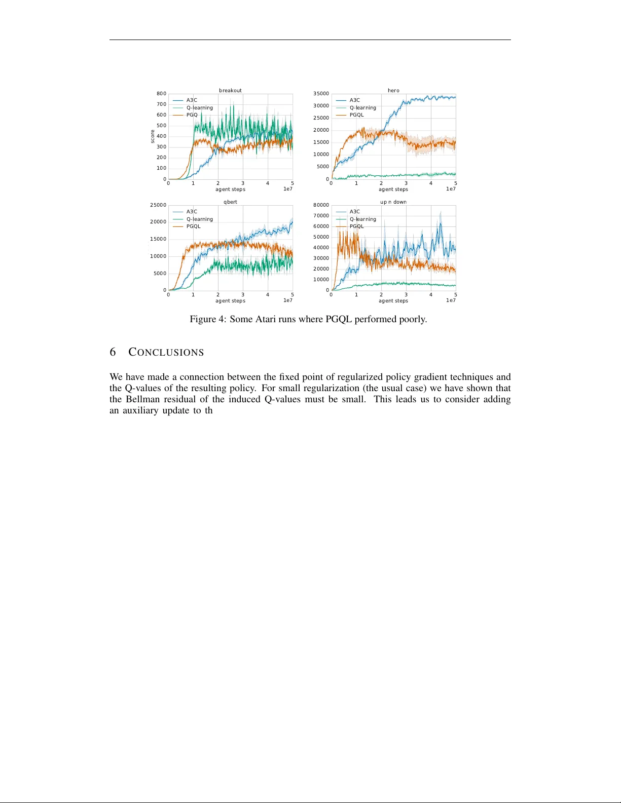
Published as a conference paper at ICLR 2017 C O M B I N I N G P O L I C Y G R A D I E N T A N D Q - L E A R N I N G Brendan O’Donoghue, R ´ emi Munos, Koray Ka vukcuoglu & V olodymyr Mnih Deepmind { bodonoghue,munos,korayk,vmnih } @google.com A B S T R AC T Policy gradient is an ef ficient technique for impro ving a polic y in a reinforcement learning setting. Howe v er , vanilla online variants are on-policy only and not able to take adv antage of of f-policy data. In this paper we describe a new technique that combines policy gradient with off-polic y Q-learning, drawing experience from a replay buf fer . This is motiv ated by making a connection between the fixed points of the regularized policy gradient algorithm and the Q-v alues. This connection allows us to estimate the Q-v alues from the action preferences of the policy , to which we apply Q-learning updates. W e refer to the new technique as ‘PGQL ’, for policy gradient and Q-learning. W e also establish an equi valenc y between action-value fitting techniques and actor-critic algorithms, sho wing that regular - ized policy gradient techniques can be interpreted as advantage function learning algorithms. W e conclude with some numerical examples that demonstrate im- prov ed data efficiency and stability of PGQL. In particular, we tested PGQL on the full suite of Atari games and achieved performance exceeding that of both asynchronous advantage actor -critic (A3C) and Q-learning. 1 I N T RO D U C T I O N In reinforcement learning an agent explores an en vironment and through the use of a reward signal learns to optimize its behavior to maximize the expected long-term return. Reinforcement learning has seen success in se veral areas including robotics (Lin, 1993; Le vine et al., 2015), computer games (Mnih et al., 2013; 2015), online advertising (Pednault et al., 2002), board games (T esauro, 1995; Silver et al., 2016), and many others. For an introduction to reinforcement learning we refer to the classic text by Sutton & Barto (1998). In this paper we consider model-free reinforcement learning, where the state-transition function is not kno wn or learned. There are many dif ferent algorithms for model-free reinforcement learning, but most fall into one of two families: action-value fitting and policy gradient techniques. Action-value techniques in v olve fitting a function, called the Q-values, that captures the expected return for taking a particular action at a particular state, and then follo wing a particular polic y there- after . T wo alternativ es we discuss in this paper are SARSA (Rummery & Niranjan, 1994) and Q-learning (W atkins, 1989), although there are many others. SARSA is an on-policy algorithm whereby the action-value function is fit to the current policy , which is then refined by being mostly greedy with respect to those action-values. On the other hand, Q-learning attempts to find the Q- values associated with the optimal policy directly and does not fit to the policy that was used to generate the data. Q-learning is an of f-policy algorithm that can use data generated by another agent or from a replay b uf fer of old experience. Under certain conditions both SARSA and Q-learning can be sho wn to conv erge to the optimal Q-values, from which we can derive the optimal policy (Sutton, 1988; Bertsekas & Tsitsiklis, 1996). In polic y gradient techniques the policy is represented explicitly and we improve the policy by updating the parameters in the direction of the gradient of the performance (Sutton et al., 1999; Silver et al., 2014; Kakade, 2001). Online policy gradient typically requires an estimate of the action-value function of the current policy . For this reason they are often referred to as actor-critic methods, where the actor refers to the policy and the critic to the estimate of the action-v alue function (K onda & Tsitsiklis, 2003). V anilla actor -critic methods are on-policy only , although some attempts hav e been made to extend them to of f-polic y data (Degris et al., 2012; Le vine & K oltun, 2013). 1 Published as a conference paper at ICLR 2017 In this paper we deriv e a link between the Q-values induced by a policy and the policy itself when the policy is the fix ed point of a regularized policy gradient algorithm (where the gradient van- ishes). This connection allo ws us to derive an estimate of the Q-values from the current policy , which we can refine using off-polic y data and Q-learning. W e show in the tabular setting that when the regularization penalty is small (the usual case) the resulting policy is close to the policy that would be found without the addition of the Q-learning update. Separately , we sho w that re gularized actor-critic methods can be interpreted as action-value fitting methods, where the Q-v alues hav e been parameterized in a particular way . W e conclude with some numerical examples that provide empirical evidence of impro ved data ef ficiency and stability of PGQL. 1 . 1 P R I O R W O R K Here we highlight various axes along which our work can be compared to others. In this paper we use entropy regularization to ensure e xploration in the policy , which is a common practice in policy gradient (W illiams & Peng, 1991; Mnih et al., 2016). An alternati ve is to use KL-di ver gence instead of entrop y as a re gularizer , or as a constraint on ho w much de viation is permitted from a prior policy (Bagnell & Schneider, 2003; Peters et al., 2010; Schulman et al., 2015; Fox et al., 2015). Natural policy gradient can also be interpreted as putting a constraint on the KL-di ver gence at each step of the policy improvement (Amari, 1998; Kakade, 2001; Pascanu & Bengio, 2013). In Sallans & Hinton (2004) the authors use a Boltzmann exploration policy over estimated Q-values which they update using TD-learning. In Heess et al. (2012) this was extended to use an actor-critic algorithm instead of TD-learning, howe ver the two updates were not combined as we have done in this paper . In Azar et al. (2012) the authors de velop an algorithm called dynamic policy programming, whereby they apply a Bellman-like update to the action-preferences of a policy , which is similar in spirit to the update we describe here. In Norouzi et al. (2016) the authors augment a maximum likelihood objectiv e with a reward in a supervised learning setting, and develop a connection that resembles the one we develop here between the policy and the Q-values. Other works hav e attempted to com- bine on and off-polic y learning, primarily using action-value fitting methods (W ang et al., 2013; Hausknecht & Stone, 2016; Lehnert & Precup, 2015), with varying degrees of success. In this paper we establish a connection between actor-critic algorithms and action-value learning algorithms. In particular we show that TD-actor -critic (K onda & Tsitsiklis, 2003) is equi valent to expected-SARSA (Sutton & Barto, 1998, Exercise 6.10) with Boltzmann exploration where the Q-values are decom- posed into advantage function and value function. The algorithm we develop extends actor-critic with a Q-learning style update that, due to the decomposition of the Q-values, resembles the update of the dueling architecture (W ang et al., 2016). Recently , the field of deep reinforcement learning, i.e. , the use of deep neural networks to represent action-values or a policy , has seen a lot of success (Mnih et al., 2015; 2016; Silver et al., 2016; Riedmiller, 2005; Lillicrap et al., 2015; V an Hasselt et al., 2016). In the examples section we use a neural network with PGQL to play the Atari games suite. 2 R E I N F O R C E M E N T L E A R N I N G W e consider the infinite horizon, discounted, finite state and action space Markov decision process, with state space S , action space A and rewards at each time period denoted by r t ∈ R . A policy π : S × A → R + is a mapping from state-action pair to the probability of taking that action at that state, so it must satisfy P a ∈A π ( s, a ) = 1 for all states s ∈ S . Any policy π induces a probability distrib ution ov er visited states, d π : S → R + (which may depend on the initial state), so the probability of seeing state-action pair ( s, a ) ∈ S × A is d π ( s ) π ( s, a ) . In reinforcement learning an ‘agent’ interacts with an en vironment o ver a number of times steps. At each time step t the agent recei ves a state s t and a re ward r t and selects an action a t from the polic y π t , at which point the agent moves to the ne xt state s t +1 ∼ P ( · , s t , a t ) , where P ( s 0 , s, a ) is the probability of transitioning from state s to state s 0 after taking action a . This continues until the agent encounters a terminal state (after which the process is typically restarted). The goal of the agent is to find a policy π that maximizes the expected total discounted return J ( π ) = E ( P ∞ t =0 γ t r t | π ) , where the e xpectation is with respect to the initial state distribution, the state-transition probabilities, and the policy , and where γ ∈ (0 , 1) is the discount factor that, loosely speaking, controls how much the agent prioritizes long-term versus short-term rew ards. Since the agent starts with no knowledge 2 Published as a conference paper at ICLR 2017 of the environment it must continually explore the state space and so will typically use a stochastic policy . Action-values. The action-v alue, or Q-value, of a particular state under policy π is the ex- pected total discounted return from taking that action at that state and following π thereafter , i.e. , Q π ( s, a ) = E ( P ∞ t =0 γ t r t | s 0 = s, a 0 = a, π ) . The v alue of state s under policy π is denoted by V π ( s ) = E ( P ∞ t =0 γ t r t | s 0 = s, π ) , which is the expected total discounted return of policy π from state s . The optimal action-value function is denoted Q ? and satisfies Q ? ( s, a ) = max π Q π ( s, a ) for each ( s, a ) . The policy that achie ves the maximum is the optimal policy π ? , with value function V ? . The advantage function is the difference between the action-value and the v alue function, i.e. , A π ( s, a ) = Q π ( s, a ) − V π ( s ) , and represents the additional expected reward of taking action a ov er the average performance of the policy from state s . Since V π ( s ) = P a π ( s, a ) Q π ( s, a ) we have the identity P a π ( s, a ) A π ( s, a ) = 0 , which simply states that the policy π has no advantage over itself. Bellman equation. The Bellman operator T π (Bellman, 1957) for policy π is defined as T π Q ( s, a ) = E s 0 ,r,b ( r ( s, a ) + γ Q ( s 0 , b )) , where the expectation is over next state s 0 ∼ P ( · , s, a ) , the reward r ( s, a ) , and the action b from policy π s 0 . The Q-value function for policy π is the fixed point of the Bellman operator for π , i.e. , T π Q π = Q π . The optimal Bellman operator T ? is defined as T ? Q ( s, a ) = E s 0 ,r ( r ( s, a ) + γ max b Q ( s 0 , b )) , where the expectation is over the next state s 0 ∼ P ( · , s, a ) , and the re ward r ( s, a ) . The optimal Q-value function is the fixed point of the optimal Bellman equation, i.e. , T ? Q ? = Q ? . Both the π -Bellman operator and the optimal Bellman operator are γ -contraction mappings in the sup-norm, i.e. , kT Q 1 − T Q 2 k ∞ ≤ γ k Q 1 − Q 2 k ∞ , for any Q 1 , Q 2 ∈ R S ×A . From this fact one can show that the fixed point of each operator is unique, and that v alue iteration conv er ges, i.e. , ( T π ) k Q → Q π and ( T ? ) k Q → Q ? from any initial Q . (Bertsekas, 2005). 2 . 1 A C T I O N - V A L U E L E A R N I N G In value based reinforcement learning we approximate the Q-values using a function approximator . W e then update the parameters so that the Q-values are as close to the fixed point of a Bellman equation as possible. If we denote by Q ( s, a ; θ ) the approximate Q-values parameterized by θ , then Q-learning updates the Q-values along direction E s,a ( T ? Q ( s, a ; θ ) − Q ( s, a ; θ )) ∇ θ Q ( s, a ; θ ) and SARSA updates the Q-v alues along direction E s,a ( T π Q ( s, a ; θ ) − Q ( s, a ; θ )) ∇ θ Q ( s, a ; θ ) . In the online setting the Bellman operator is approximated by sampling and bootstrapping, whereby the Q-values at an y state are updated using the Q-values from the next visited state. Exploration is achie ved by not always taking the action with the highest Q-value at each time step. One common technique called ‘epsilon greedy’ is to sample a random action with probability  > 0 , where  starts high and decreases ov er time. Another popular technique is ‘Boltzmann explo- ration’, where the policy is given by the softmax over the Q-values with a temperature T , i.e. , π ( s, a ) = exp( Q ( s, a ) /T ) / P b exp( Q ( s, b ) /T ) , where it is common to decrease the temperature ov er time. 2 . 2 P O L I C Y G R A D I E N T Alternativ ely , we can parameterize the policy directly and attempt to improve it via gradient ascent on the performance J . The policy gradient theorem (Sutton et al., 1999) states that the gradient of J with respect to the parameters of the policy is giv en by ∇ θ J ( π ) = E s,a Q π ( s, a ) ∇ θ log π ( s, a ) , (1) where the expectation is over ( s, a ) with probability d π ( s ) π ( s, a ) . In the original deriv ation of the policy gradient theorem the expectation is over the discounted distrib ution of states, i.e. , over d π ,s 0 γ ( s ) = P ∞ t =0 γ t P r { s t = s | s 0 , π } . Howe ver , the gradient update in that case will assign a low 3 Published as a conference paper at ICLR 2017 weight to states that take a long time to reach and can therefore hav e poor empirical performance. In practice the non-discounted distribution of states is frequently used instead. In certain cases this is equiv alent to maximizing the average ( i.e. , non-discounted) polic y performance, e ven when Q π uses a discount factor (Thomas, 2014). Throughout this paper we will use the non-discounted distribution of states. In the online case it is common to add an entropy regularizer to the gradient in order to prevent the policy becoming deterministic. This ensures that the agent will explore continually . In that case the (batch) update becomes ∆ θ ∝ E s,a Q π ( s, a ) ∇ θ log π ( s, a ) + α E s ∇ θ H π ( s ) , (2) where H π ( s ) = − P a π ( s, a ) log π ( s, a ) denotes the entropy of policy π , and α > 0 is the reg- ularization penalty parameter . Throughout this paper we will make use of entropy regularization, howe ver many of the results are true for other choices of regularizers with only minor modification, e.g . , KL-diver gence. Note that equation (2) requires exact knowledge of the Q-v alues. In practice they can be estimated, e.g. , by the sum of discounted re wards along an observed trajectory (Williams, 1992), and the policy gradient will still perform well (K onda & Tsitsiklis, 2003). 3 R E G U L A R I Z E D P O L I C Y G R A D I E N T A L G O R I T H M In this section we derive a relationship between the policy and the Q-values when using a regularized policy gradient algorithm. This allows us to transform a polic y into an estimate of the Q-v alues. W e then show that for small regularization the Q-v alues induced by the policy at the fixed point of the algorithm hav e a small Bellman error in the tabular case. 3 . 1 T A B U L A R C A S E Consider the fixed points of the entropy regularized policy gradient update (2). Let us define f ( θ ) = E s,a Q π ( s, a ) ∇ θ log π ( s, a ) + α E s ∇ θ H ( π s ) , and g s ( π ) = P a π ( s, a ) for each s . A fixed point is one where we can no longer update θ in the direction of f ( θ ) without violating one of the constraints g s ( π ) = 1 , i.e. , where f ( θ ) is in the span of the v ectors {∇ θ g s ( π ) } . In other words, any fixed point must satisfy f ( θ ) = P s λ s ∇ θ g s ( π ) , where for each s the Lagrange multiplier λ s ∈ R ensures that g s ( π ) = 1 . Substituting in terms to this equation we obtain E s,a ( Q π ( s, a ) − α log π ( s, a ) − c s ) ∇ θ log π ( s, a ) = 0 , (3) where we have absorbed all constants into c ∈ R |S | . Any solution π to this equation is strictly positiv e element-wise since it must lie in the domain of the entropy function. In the tabular case π is represented by a single number for each state and action pair and the gradient of the policy with respect to the parameters is the indicator function, i.e. , ∇ θ ( t,b ) π ( s, a ) = 1 ( t,b )=( s,a ) . From this we obtain Q π ( s, a ) − α log π ( s, a ) − c s = 0 for each s (assuming that the measure d π ( s ) > 0 ). Multiplying by π ( a, s ) and summing ov er a ∈ A we get c s = αH π ( s ) + V π ( s ) . Substituting c into equation (3) we hav e the follo wing formulation for the policy: π ( s, a ) = exp( A π ( s, a ) /α − H π ( s )) , (4) for all s ∈ S and a ∈ A . In other words, the policy at the fixed point is a softmax over the advantage function induced by that policy , where the regularization parameter α can be interpreted as the temperature. Therefore, we can use the policy to deriv e an estimate of the Q-v alues, ˜ Q π ( s, a ) = ˜ A π ( s, a ) + V π ( s ) = α (log π ( s, a ) + H π ( s )) + V π ( s ) . (5) W ith this we can re write the gradient update (2) as ∆ θ ∝ E s,a ( Q π ( s, a ) − ˜ Q π ( s, a )) ∇ θ log π ( s, a ) , (6) since the update is unchanged by per-state constant offsets. When the policy is parameterized as a softmax, i.e. , π ( s, a ) = exp( W ( s, a )) / P b exp W ( s, b ) , the quantity W is sometimes referred to as the action-preferences of the policy (Sutton & Barto, 1998, Chapter 6.6). Equation (4) states that the action preferences are equal to the Q-values scaled by 1 /α , up to an additi ve per -state constant. 4 Published as a conference paper at ICLR 2017 3 . 2 G E N E R A L C A S E Consider the following optimization problem: minimize E s,a ( q ( s, a ) − α log π ( s, a )) 2 subject to P a π ( s, a ) = 1 , s ∈ S (7) ov er variable θ which parameterizes π , where we consider both the measure in the expectation and the values q ( s, a ) to be independent of θ . The optimality condition for this problem is E s,a ( q ( s, a ) − α log π ( s, a ) + c s ) ∇ θ log π ( s, a ) = 0 , where c ∈ R |S | is the Lagrange multiplier associated with the constraint that the policy sum to one at each state. Comparing this to equation (3), we see that if q = Q π and the measure in the e xpectation is the same then they describe the same set of fixed points. This suggests an interpretation of the fixed points of the regularized policy gradient as a regression of the log-policy onto the Q-v alues. In the general case of using an approximation architecture we can interpret equation (3) as indicating that the error between Q π and ˜ Q π is orthogonal to ∇ θ i log π for each i , and so cannot be reduced further by changing the parameters, at least locally . In this case equation (4) is unlikely to hold at a solution to (3), howev er with a good approximation architecture it may hold approximately , so that the we can deriv e an estimate of the Q-values from the policy using equation (5). W e will use this estimate of the Q-values in the ne xt section. 3 . 3 C O N N E C T I O N T O A C T I O N - V A L U E M E T H O D S The previous section made a connection between regularized policy gradient and a regression onto the Q-values at the fixed point. In this section we go one step further, showing that actor -critic methods can be interpreted as action-value fitting methods, where the exact method depends on the choice of critic. Actor -critic methods. Consider an agent using an actor -critic method to learn both a policy π and a value function V . At any iteration k , the value function V k has parameters w k , and the policy is of the form π k ( s, a ) = exp( W k ( s, a ) /α ) / X b exp( W k ( s, b ) /α ) , (8) where W k is parameterized by θ k and α > 0 is the entropy regularization penalty . In this case ∇ θ log π k ( s, a ) = (1 /α )( ∇ θ W k ( s, a ) − P b π ( s, b ) ∇ θ W k ( s, b )) . Using equation (6) the parame- ters are updated as ∆ θ ∝ E s,a δ ac ( ∇ θ W k ( s, a ) − X b π k ( s, b ) ∇ θ W k ( s, b )) , ∆ w ∝ E s,a δ ac ∇ w V k ( s ) (9) where δ ac is the critic minus baseline term, which depends on the variant of actor-critic being used (see the remark below). Action-value methods. Compare this to the case where an agent is learning Q-values with a du- eling architecture (W ang et al., 2016), which at iteration k is giv en by Q k ( s, a ) = Y k ( s, a ) − X b µ ( s, b ) Y k ( s, b ) + V k ( s ) , where µ is a probability distribution, Y k is parameterized by θ k , V k is parameterized by w k , and the exploration polic y is Boltzmann with temperature α , i.e. , π k ( s, a ) = exp( Y k ( s, a ) /α ) / X b exp( Y k ( s, b ) /α ) . (10) In action value fitting methods at each iteration the parameters are updated to reduce some error , where the update is giv en by ∆ θ ∝ E s,a δ av ( ∇ θ Y k ( s, a ) − X b µ ( s, b ) ∇ θ Y k ( s, b )) , ∆ w ∝ E s,a δ av ∇ w V k ( s ) (11) where δ av is the action-value err or term and depends on which algorithm is being used (see the remark below). 5 Published as a conference paper at ICLR 2017 Equivalence. The two policies (8) and (10) are identical if W k = Y k for all k . Since X 0 and Y 0 can be initialized and parameterized in the same way , and assuming the two value function estimates are initialized and parameterized in the same way , all that remains is to sho w that the updates in equations (11) and (9) are identical. Comparing the two, and assuming that δ ac = δ av (see remark), we see that the only difference is that the measure is not fixed in (9), but is equal to the current policy and therefore changes after each update. Replacing µ in (11) with π k makes the updates identical, in which case W k = Y k at all iterations and the two policies (8) and (10) are always the same. In other words, the slightly modified action-value method is equiv alent to an actor-critic policy gradient method, and vice-versa (modulo using the non-discounted distribu- tion of states, as discussed in § 2.2). In particular, regularized policy gradient methods can be inter- preted as adv antage function learning techniques (Baird III, 1993), since at the optimum the quantity W ( s, a ) − P b π ( s, b ) W ( s, b ) = α (log π ( s, a ) + H π ( s )) will be equal to the advantage function values in the tab ular case. Remark. In SARSA (Rummery & Niranjan, 1994) we set δ av = r ( s, a ) + γ Q ( s 0 , b ) − Q ( s, a ) , where b is the action selected at state s 0 , which would be equiv alent to using a bootstrap critic in equation (6) where Q π ( s, a ) = r ( s, a ) + γ ˜ Q ( s 0 , b ) . In expected-SARSA (Sutton & Barto, 1998, Exercise 6.10), (V an Seijen et al., 2009)) we take the expectation o ver the Q-values at the next state, so δ av = r ( s, a ) + γ V ( s 0 ) − Q ( s, a ) . This is equi valent to TD-actor-critic (K onda & Tsitsiklis, 2003) where we use the value function to provide the critic, which is giv en by Q π = r ( s, a ) + γ V ( s 0 ) . In Q-learning (W atkins, 1989) δ av = r ( s, a ) + γ max b Q ( s 0 , b ) − Q ( s, a ) , which would be equiv alent to using an optimizing critic that bootstraps using the max Q-v alue at the next state, i.e. , Q π ( s, a ) = r ( s, a ) + γ max b ˜ Q π ( s 0 , b ) . In REINFORCE the critic is the Monte Carlo return from that state on, i.e. , Q π ( s, a ) = ( P ∞ t =0 γ t r t | s 0 = s, a 0 = a ) . If the return trace is truncated and a bootstrap is performed after n -steps, this is equi v alent to n -step SARSA or n -step Q-learning, depending on the form of the bootstrap (Peng & W illiams, 1996). 3 . 4 B E L L M A N R E S I D U A L In this section we show that kT ? Q π α − Q π α k → 0 with decreasing regularization penalty α , where π α is the policy defined by (4) and Q π α is the corresponding Q-value function, both of which are functions of α . W e shall show that it conv erges to zero by bounding the sequence below by zero and above with a sequence that conv erges to zero. First, we have that T ? Q π α ≥ T π α Q π α = Q π α , since T ? is greedy with respect to the Q-v alues. So T ? Q π α − Q π α ≥ 0 . Now , to bound from above we need the fact that π α ( s, a ) = exp( Q π α ( s, a ) /α ) / P b exp( Q π α ( s, b ) /α ) ≤ exp(( Q π α ( s, a ) − max c Q π α ( s, c )) /α ) . Using this we have 0 ≤ T ? Q π α ( s, a ) − Q π α ( s, a ) = T ? Q π α ( s, a ) − T π α Q π α ( s, a ) = E s 0 (max c Q π α ( s 0 , c ) − P b π α ( s 0 , b ) Q π α ( s 0 , b )) = E s 0 P b π α ( s 0 , b )(max c Q π α ( s 0 , c ) − Q π α ( s 0 , b )) ≤ E s 0 P b exp(( Q π α ( s 0 , b ) − Q π α ( s 0 , b ? )) /α )(max c Q π α ( s 0 , c ) − Q π α ( s 0 , b )) = E s 0 P b f α (max c Q π α ( s 0 , c ) − Q π α ( s 0 , b )) , where we define f α ( x ) = x exp( − x/α ) . T o conclude our proof we use the fact that f α ( x ) ≤ sup x f α ( x ) = f α ( α ) = α e − 1 , which yields 0 ≤ T ? Q π α ( s, a ) − Q π α ( s, a ) ≤ |A| α e − 1 for all ( s, a ) , and so the Bellman residual conv erges to zero with decreasing α . In other words, for small enough α (which is the regime we are interested in) the Q-values induced by the policy (4) will hav e a small Bellman residual. Moreov er , this implies that lim α → 0 Q π α = Q ? , as one might expect. 4 P G Q L In this section we introduce the main contrib ution of the paper , which is a technique to combine pol- icy gradient with Q-learning. W e call our technique ‘PGQL ’, for policy gradient and Q-learning. In the pre vious section we showed that the Bellman residual is small at the fixed point of a re gularized 6 Published as a conference paper at ICLR 2017 policy gradient algorithm when the regularization penalty is sufficiently small. This suggests adding an auxiliary update where we explicitly attempt to reduce the Bellman residual as estimated from the policy , i.e. , a hybrid between policy gradient and Q-learning. W e first present the technique in a batch update setting, with a perfect knowledge of Q π ( i.e. , a perfect critic). Later we discuss the practical implementation of the technique in a reinforcement learning setting with function approximation, where the agent generates experience from interacting with the en vironment and needs to estimate a critic simultaneously with the policy . 4 . 1 P G Q L U P D A T E Define the estimate of Q using the policy as ˜ Q π ( s, a ) = α (log π ( s, a ) + H π ( s )) + V ( s ) , (12) where V has parameters w and is not necessarily V π as it was in equation (5). In (2) it was unneces- sary to estimate the constant since the update was in variant to constant offsets, although in practice it is often estimated for use in a variance reduction technique (W illiams, 1992; Sutton et al., 1999). Since we kno w that at the fix ed point the Bellman residual will be small for small α , we can consider updating the parameters to reduce the Bellman residual in a fashion similar to Q-learning, i.e . , ∆ θ ∝ E s,a ( T ? ˜ Q π ( s, a ) − ˜ Q π ( s, a )) ∇ θ log π ( s, a ) , ∆ w ∝ E s,a ( T ? ˜ Q π ( s, a ) − ˜ Q π ( s, a )) ∇ w V ( s ) . (13) This is Q-learning applied to a particular form of the Q-v alues, and can also be interpreted as an actor-critic algorithm with an optimizing (and therefore biased) critic. The full scheme simply combines two updates to the policy , the regularized policy gradient update (2) and the Q-learning update (13). Assuming we hav e an architecture that provides a policy π , a value function estimate V , and an action-value critic Q π , then the parameter updates can be written as (suppressing the ( s, a ) notation) ∆ θ ∝ (1 − η ) E s,a ( Q π − ˜ Q π ) ∇ θ log π + η E s,a ( T ? ˜ Q π − ˜ Q π ) ∇ θ log π , ∆ w ∝ (1 − η ) E s,a ( Q π − ˜ Q π ) ∇ w V + η E s,a ( T ? ˜ Q π − ˜ Q π ) ∇ w V , (14) here η ∈ [0 , 1] is a weighting parameter that controls ho w much of each update we apply . In the case where η = 0 the above scheme reduces to entropy regularized policy gradient. If η = 1 then it becomes a v ariant of (batch) Q-learning with an architecture similar to the dueling architecture (W ang et al., 2016). Intermediate values of η produce a hybrid between the two. Examining the update we see that two error terms are trading of f. The first term encourages consistency with critic, and the second term encourages optimality ov er time. Howe ver , since we know that under standard policy gradient the Bellman residual will be small, then it follows that adding a term that reduces that error should not make much difference at the fixed point. That is, the updates should be complementary , pointing in the same general direction, at least far aw ay from a fixed point. This update can also be interpreted as an actor-critic update where the critic is given by a weighted combination of a standard critic and an optimizing critic. Y et another interpretation of the update is a combination of expected-SARSA and Q-learning, where the Q-values are parameterized as the sum of an advantage function and a v alue function. 4 . 2 P R A C T I C A L I M P L E M E N TA T I O N The updates presented in (14) are batch updates, with an exact critic Q π . In practice we want to run this scheme online, with an estimate of the critic, where we don’t necessarily apply the policy gradient update at the same time or from same data source as the Q-learning update. Our proposal scheme is as follows. One or more agents interact with an environment, encountering states and re wards and performing on-policy updates of (shared) parameters using an actor-critic algorithm where both the policy and the critic are being updated online. Each time an agent receiv es new data from the en vironment it writes it to a shared replay memory buf fer . Periodically a separate learner process samples from the replay buffer and performs a step of Q-learning on the parameters of the policy using (13). This scheme has sev eral advantages. The critic can accumulate the Monte 7 Published as a conference paper at ICLR 2017 S T (a) Grid world. 0 200 400 600 800 1000 1200 1400 agent steps 0.0 0.1 0.2 0.3 0.4 0.5 0.6 expected discounted return from start Actor-critic Q-learning PGQL (b) Performance versus agent steps in grid world. Figure 1: Grid world experiment. Carlo return ov er many time periods, allowing us to spread the influence of a re ward receiv ed in the future backw ards in time. Furthermore, the replay buf fer can be used to store and replay ‘important’ past e xperiences by prioritizing those samples (Schaul et al., 2015). The use of the replay b uf fer can help to reduce problems associated with correlated training data, as generated by an agent explor - ing an environment where the states are likely to be similar from one time step to the next. Also the use of replay can act as a kind of regularizer , pre venting the policy from moving too far from satisfying the Bellman equation, thereby improving stability , in a similar sense to that of a policy ‘trust-region’ (Schulman et al., 2015). Moreov er , by batching up replay samples to update the net- work we can lev erage GPUs to perform the updates quickly , this is in comparison to pure policy gradient techniques which are generally implemented on CPU (Mnih et al., 2016). Since we perform Q-learning using samples from a replay buf fer that were generated by a old polic y we are performing (slightly) off-polic y learning. Ho wev er , Q-learning is known to con ver ge to the optimal Q-values in the off-polic y tabular case (under certain conditions) (Sutton & Barto, 1998), and has sho wn good performance of f-policy in the function approximation case (Mnih et al., 2013). 4 . 3 M O D I FI E D FI X E D P O I N T The PGQL updates in equation (14) hav e modified the fixed point of the algorithm, so the analysis of § 3 is no longer v alid. Considering the tabular case once again, it is still the case that the policy π ∝ exp( ˜ Q π /α ) as before, where ˜ Q π is defined by (12), howe ver where previously the fixed point satisfied ˜ Q π = Q π , with Q π corresponding to the Q-values induced by π , no w we hav e ˜ Q π = (1 − η ) Q π + η T ? ˜ Q π , (15) Or equiv alently , if η < 1 , we have ˜ Q π = (1 − η ) P ∞ k =0 η k ( T ? ) k Q π . In the appendix we show that k ˜ Q π − Q π k → 0 and that kT ? Q π − Q π k → 0 with decreasing α in the tabular case. That is, for small α the induced Q-v alues and the Q-values estimated from the policy are close, and we still have the guarantee that in the limit the Q-values are optimal. In other words, we hav e not perturbed the policy v ery much by the addition of the auxiliary update. 5 N U M E R I C A L E X P E R I M E N T S 5 . 1 G R I D W O R L D In this section we discuss the results of running PGQL on a toy 4 by 6 grid world, as sho wn in Figure 1a. The agent always begins in the square marked ‘S’ and the episode continues until it reaches the square marked ‘T’, upon which it receiv es a reward of 1 . All other times it receiv es no reward. For this experiment we chose re gularization parameter α = 0 . 001 and discount factor γ = 0 . 95 . Figure 1b sho ws the performance traces of three different agents learning in the grid world, running from the same initial random seed. The lines sho w the true expected performance of the policy 8 Published as a conference paper at ICLR 2017 Figure 2: PGQL network augmentation. from the start state, as calculated by value iteration after each update. The blue-line is standard TD-actor-critic (K onda & Tsitsiklis, 2003), where we maintain an estimate of the v alue function and use that to generate an estimate of the Q-values for use as the critic. The green line is Q-learning where at each step an update is performed using data drawn from a replay b uf fer of prior experience and where the Q-v alues are parameterized as in equation (12). The polic y is a softmax over the Q-value estimates with temperature α . The red line is PGQL, which at each step first performs the TD-actor-critic update, then performs the Q-learning update as in (14). The grid world was totally deterministic, so the step size could be large and was chosen to be 1 . A step-size any larger than this made the pure actor-critic agent fail to learn, b ut both PGQL and Q-learning could handle some increase in the step-size, possibly due to the stabilizing ef fect of using replay . It is clear that PGQL outperforms the other two. At any point along the x-axis the agents have seen the same amount of data, which would indicate that PGQL is more data efficient than either of the vanilla methods since it has the highest performance at practically e very point. 5 . 2 A TA R I W e tested our algorithm on the full suite of Atari benchmarks (Bellemare et al., 2012), using a neural network to parameterize the policy . In figure 2 we show how a policy network can be augmented with a parameterless additional layer which outputs the Q-v alue estimate. W ith the exception of the extra layer, the architecture and parameters were chosen to exactly match the asynchronous advantage actor-critic (A3C) algorithm presented in Mnih et al. (2016), which in turn reused many of the settings from Mnih et al. (2015). Specifically we used the exact same learning rate, number of workers, entropy penalty , bootstrap horizon, and network architecture. This allows a f air comparison between A3C and PGQL, since the only dif ference is the addition of the Q-learning step. Our technique augmented A3C with the following change: After each actor-learner has accumulated the gradient for the policy update, it performs a single step of Q-learning from replay data as described in equation (13), where the minibatch size was 32 and the Q-learning learning rate was chosen to be 0 . 5 times the actor-critic learning rate (we mention learning rate ratios rather than choice of η in (14) because the updates happen at different frequencies and from different data sources). Each actor-learner thread maintained a replay buffer of the last 100 k transitions seen by that thread. W e ran the learning for 50 million agent steps ( 200 million Atari frames), as in (Mnih et al., 2016). In the results we compare against both A3C and a variant of asynchronous deep Q-learning. The changes we made to Q-learning are to make it similar to our method, with some tuning of the hyper - parameters for performance. W e use the exact same network, the exploration policy is a softmax ov er the Q-v alues with a temperature of 0 . 1 , and the Q-v alues are parameterized as in equation (12) ( i.e. , similar to the dueling architecture (W ang et al., 2016)), where α = 0 . 1 . The Q-value updates are performed every 4 steps with a minibatch of 32 (roughly 5 times more frequently than PGQL). For each method, all games used identical hyper -parameters. The results across all games are giv en in table 3 in the appendix. All scores ha ve been normal- ized by subtracting the average score achiev ed by an agent that takes actions uniformly at random. 9 Published as a conference paper at ICLR 2017 Each game was tested 5 times per method with the same hyper-parameters but with different ran- dom seeds. The scores presented correspond to the best score obtained by any run from a random start ev aluation condition (Mnih et al., 2016). Overall, PGQL performed best in 34 games, A3C performed best in 7 games, and Q-learning was best in 10 games. In 6 games two or more methods tied. In tables 1 and 2 we giv e the mean and median normalized scores as percentage of an expert human normalized score across all games for each tested algorithm from random and human-start conditions respectively . In a human-start condition the agent takes over control of the game from randomly selected human-play starting points, which generally leads to lower performance since the agent may not have found itself in that state during training. In both cases, PGQL has both the highest mean and median, and the median score exceeds 100%, the human performance threshold. It is worth noting that PGQL was the worst performer in only one game, in cases where it was not the outright winner it was generally somewhere in between the performance of the other two algorithms. Figure 3 shows some sample traces of games where PGQL was the best performer . In these cases PGQL has far better data efficiency than the other methods. In figure 4 we show some of the games where PGQL under-performed. In practically every case where PGQL did not perform well it had better data efficiency early on in the learning, but performance saturated or collapsed. W e hypothesize that in these cases the policy has reached a local optimum, or over -fit to the early data, and might perform better were the hyper-parameters to be tuned. A3C Q-learning PGQL Mean 636.8 756.3 877.2 Median 107.3 58.9 145.6 T able 1: Mean and median normalized scores for the Atari suite from random starts, as a percentage of human normalized score. A3C Q-learning PGQL Mean 266.6 246.6 416.7 Median 58.3 30.5 103.3 T able 2: Mean and median normalized scores for the Atari suite from human starts, as a percentage of human normalized score. 0 1 2 3 4 5 agent steps 1e7 0 2000 4000 6000 8000 10000 12000 score assault A3C Q-learning PGQL 0 1 2 3 4 5 agent steps 1e7 0 2000 4000 6000 8000 10000 12000 14000 16000 score battle zone A3C Q-learning PGQL 0 1 2 3 4 5 agent steps 1e7 0 2000 4000 6000 8000 10000 12000 score chopper command A3C Q-learning PGQL 0 1 2 3 4 5 agent steps 1e7 0 20000 40000 60000 80000 100000 score yars revenge A3C Q-learning PGQL Figure 3: Some Atari runs where PGQL performed well. 10 Published as a conference paper at ICLR 2017 0 1 2 3 4 5 agent steps 1e7 0 100 200 300 400 500 600 700 800 score breakout A3C Q-learning PGQ 0 1 2 3 4 5 agent steps 1e7 0 5000 10000 15000 20000 25000 30000 35000 score hero A3C Q-learning PGQL 0 1 2 3 4 5 agent steps 1e7 0 5000 10000 15000 20000 25000 score qbert A3C Q-learning PGQL 0 1 2 3 4 5 agent steps 1e7 0 10000 20000 30000 40000 50000 60000 70000 80000 score up n down A3C Q-learning PGQL Figure 4: Some Atari runs where PGQL performed poorly . 6 C O N C L U S I O N S W e have made a connection between the fixed point of regularized policy gradient techniques and the Q-values of the resulting policy . For small regularization (the usual case) we have shown that the Bellman residual of the induced Q-values must be small. This leads us to consider adding an auxiliary update to the policy gradient which is related to the Bellman residual e valuated on a transformation of the policy . This update can be performed off-polic y , using stored experience. W e call the resulting method ‘PGQL ’, for policy gradient and Q-learning. Empirically , we observe better data efficienc y and stability of PGQL when compared to actor-critic or Q-learning alone. W e verified the performance of PGQL on a suite of Atari g ames, where we parameterize the polic y using a neural network, and achie ved performance e xceeding that of both A3C and Q-learning. 7 A C K N O W L E D G M E N T S W e thank Joseph Modayil for many comments and suggestions on the paper , and Hubert Soyer for help with performance e valuation. W e would also like to thank the anonymous revie wers for their constructiv e feedback. 11 Published as a conference paper at ICLR 2017 R E F E R E N C E S Shun-Ichi Amari. Natural gradient works ef ficiently in learning. Neural computation , 10(2):251– 276, 1998. Mohammad Gheshlaghi Azar , V icenc ¸ G ´ omez, and Hilbert J Kappen. Dynamic polic y programming. Journal of Mac hine Learning Resear c h , 13(Nov):3207–3245, 2012. J Andrew Bagnell and Jef f Schneider . Cov ariant policy search. In IJCAI , 2003. Leemon C Baird III. Advantage updating. T echnical Report WL-TR-93-1146, Wright-Patterson Air Force Base Ohio: Wright Laboratory , 1993. Marc G Bellemare, Y av ar Naddaf, Joel V eness, and Michael Bowling. The arcade learning en vi- ronment: An ev aluation platform for general agents. Journal of Artificial Intelligence Researc h , 2012. Richard Bellman. Dynamic pr ogramming . Princeton Uni versity Press, 1957. Dimitri P Bertsekas. Dynamic pr ogramming and optimal contr ol , v olume 1. Athena Scientific, 2005. Dimitri P . Bertsekas and John N. Tsitsiklis. Neur o-Dynamic Pr ogr amming . Athena Scientific, 1996. Thomas Degris, Martha White, and Richard S Sutton. Off-policy actor -critic. 2012. Roy Fox, Ari Pakman, and Naftali T ishby . T aming the noise in reinforcement learning via soft updates. arXi v preprint arXi v:1207.4708, 2015. Matthew Hausknecht and Peter Stone. On-policy vs. off-polic y updates for deep reinforcement learning. Deep Reinforcement Learning: Frontiers and Challenges, IJ CAI 2016 W orkshop, 2016. Nicolas Heess, David Silver , and Y ee Whye T eh. Actor-critic reinforcement learning with energy- based policies. In JMLR: W orkshop and Confer ence Pr oceedings 24 , pp. 43–57, 2012. Sham Kakade. A natural policy gradient. In Advances in Neural Information Pr ocessing Systems , volume 14, pp. 1531–1538, 2001. V ijay R Konda and John N Tsitsiklis. On actor-critic algorithms. SIAM Journal on Contr ol and Optimization , 42(4):1143–1166, 2003. Lucas Lehnert and Doina Precup. Policy gradient methods for off-policy control. arXiv preprint arXiv:1512.04105, 2015. Serge y Levine and Vladlen K oltun. Guided policy search. In Pr oceedings of the 30th International Confer ence on Machine Learning (ICML) , pp. 1–9, 2013. Serge y Le vine, Chelsea Finn, T revor Darrell, and Pieter Abbeel. End-to-end training of deep visuo- motor policies. arXi v preprint arXi v:1504.00702, 2015. T imothy P Lillicrap, Jonathan J Hunt, Alexander Pritzel, Nicolas Heess, T om Erez, Y uval T assa, David Silver , and Daan W ierstra. Continuous control with deep reinforcement learning. arXiv preprint arXiv:1509.02971, 2015. Long-Ji Lin. Reinforcement learning for robots using neural networks. T echnical report, DTIC Document, 1993. V olodymyr Mnih, K oray Kavukcuoglu, David Silver , Alex Graves, Ioannis Antonoglou, Daan W ier- stra, and Martin Riedmiller . Playing atari with deep reinforcement learning. In NIPS Deep Learn- ing W orkshop . 2013. V olodymyr Mnih, K oray Kavukcuoglu, David Silver , Andrei A. Rusu, Joel V eness, Marc G. Bellemare, Alex Grav es, Martin Riedmiller , Andreas K. Fidjeland, Georg Ostrovski, Stig Pe- tersen, Charles Beattie, Amir Sadik, Ioannis Antonoglou, Helen King, Dharshan Kumaran, Daan W ierstra, Shane Legg, and Demis Hassabis. Human-le vel control through deep reinforcement learning. Natur e , 518(7540):529–533, 02 2015. URL http://dx.doi.org/10.1038/ nature14236 . 12 Published as a conference paper at ICLR 2017 V olodymyr Mnih, Adria Puigdomenech Badia, Mehdi Mirza, Alex Graves, T imothy P Lillicrap, Tim Harley , Da vid Silver , and Koray Kavukcuoglu. Asynchronous methods for deep reinforcement learning. arXiv pr eprint arXiv:1602.01783 , 2016. Mohammad Norouzi, Samy Bengio, Zhifeng Chen, Navdeep Jaitly , Mike Schuster, Y onghui W u, and Dale Schuurmans. Re ward augmented maximum likelihood for neural structured prediction. arXiv preprint arXi v:1609.00150, 2016. Razvan Pascanu and Y oshua Bengio. Revisiting natural gradient for deep networks. arXiv preprint arXiv:1301.3584, 2013. Edwin Pednault, Naoki Abe, and Bianca Zadrozny . Sequential cost-sensitive decision making with reinforcement learning. In Pr oceedings of the eighth ACM SIGKDD international confer ence on Knowledge discovery and data mining , pp. 259–268. A CM, 2002. Jing Peng and Ronald J Williams. Incremental multi-step Q-learning. Machine Learning , 22(1-3): 283–290, 1996. Jan Peters, Katharina M ¨ ulling, and Y asemin Altun. Relative entropy policy search. In AAAI . Atlanta, 2010. Martin Riedmiller . Neural fitted Q iteration–first experiences with a data efficient neural reinforce- ment learning method. In Machine Learning: ECML 2005 , pp. 317–328. Springer Berlin Heidel- berg, 2005. Gavin A Rummery and Mahesan Niranjan. On-line Q-learning using connectionist systems. 1994. Brian Sallans and Geoffre y E Hinton. Reinforcement learning with factored states and actions. Journal of Mac hine Learning Resear c h , 5(Aug):1063–1088, 2004. T om Schaul, John Quan, Ioannis Antonoglou, and David Silver . Prioritized experience replay . arXiv preprint arXiv:1511.05952, 2015. John Schulman, Sergey Levine, Pieter Abbeel, Michael Jordan, and Philipp Moritz. Trust region policy optimization. In Pr oceedings of The 32nd International Confer ence on Machine Learning , pp. 1889–1897, 2015. David Silver , Guy Lev er , Nicolas Heess, Thomas Degris, Daan W ierstra, and Martin Riedmiller . Deterministic polic y gradient algorithms. In Pr oceedings of the 31st International Confer ence on Machine Learning (ICML) , pp. 387–395, 2014. David Silver , Aja Huang, Chris J Maddison, Arthur Guez, Laurent Sifre, George V an Den Driessche, Julian Schrittwieser , Ioannis Antonoglou, V eda Panneershelvam, Marc Lanctot, et al. Mastering the game of go with deep neural networks and tree search. Nature , 529(7587):484–489, 2016. R. Sutton and A. Barto. Reinfor cement Learning: an Intr oduction . MIT Press, 1998. Richard S Sutton. Learning to predict by the methods of temporal dif ferences. Machine learning , 3 (1):9–44, 1988. Richard S Sutton, David A McAllester, Satinder P Singh, Y ishay Mansour , et al. Policy gradient methods for reinforcement learning with function approximation. In Advances in Neural Infor- mation Pr ocessing Systems , v olume 99, pp. 1057–1063, 1999. Gerald T esauro. T emporal difference learning and TD-Gammon. Communications of the ACM , 38 (3):58–68, 1995. Philip Thomas. Bias in natural actor -critic algorithms. In Proceedings of The 31st International Confer ence on Machine Learning , pp. 441–448, 2014. Hado V an Hasselt, Arthur Guez, and David Silver . Deep reinforcement learning with double Q- learning. In Pr oceedings of the Thirtieth AAAI Conference on Artificial Intelligence (AAAI-16) , pp. 2094–2100, 2016. 13 Published as a conference paper at ICLR 2017 Harm V an Seijen, Hado V an Hasselt, Shimon Whiteson, and Marco W iering. A theoretical and em- pirical analysis of expected sarsa. In 2009 IEEE Symposium on Adaptive Dynamic Pr ogramming and Reinfor cement Learning , pp. 177–184. IEEE, 2009. Y in-Hao W ang, Tzuu-Hseng S Li, and Chih-Jui Lin. Backward q-learning: The combination of sarsa algorithm and q-learning. Engineering Applications of Artificial Intelligence , 26(9):2184–2193, 2013. Ziyu W ang, T om Schaul, Matteo Hessel, Hado van Hasselt, Marc Lanctot, and Nando de Freitas. Dueling network architectures for deep reinforcement learning. In Pr oceedings of the 33r d Inter- national Confer ence on Machine Learning (ICML) , pp. 1995–2003, 2016. Christopher John Cornish Hellaby W atkins. Learning fr om delayed r ewar ds . PhD thesis, Uni versity of Cambridge England, 1989. Ronald J W illiams. Simple statistical gradient-following algorithms for connectionist reinforcement learning. Machine learning , 8(3-4):229–256, 1992. Ronald J W illiams and Jing Peng. Function optimization using connectionist reinforcement learning algorithms. Connection Science , 3(3):241–268, 1991. A P G Q L B E L L M A N R E S I D U A L Here we demonstrate that in the tabular case the Bellman residual of the induced Q-values for the PGQL updates of (14) con ver ges to zero as the temperature α decreases, which is the same guarantee as vanilla regularized policy gradient (2). W e will use the notation that π α is the policy at the fixed point of PGQL updates (14) for some α , i.e. , π α ∝ exp( ˜ Q π α ) , with induced Q-value function Q π α . First, note that we can apply the same argument as in § 3.4 to show that lim α → 0 kT ? ˜ Q π α − T π α ˜ Q π α k = 0 (the only dif ference is that we lack the property that ˜ Q π α is the fixed point of T π α ). Secondly , from equation (15) we can write ˜ Q π α − Q π α = η ( T ? ˜ Q π α − Q π α ) . Combining these two facts we ha ve k ˜ Q π α − Q π α k = η kT ? ˜ Q π α − Q π α k = η kT ? ˜ Q π α − T π α ˜ Q π α + T π α ˜ Q π α − Q π α k ≤ η ( kT ? ˜ Q π α − T π α ˜ Q π α k + kT π α ˜ Q π α − T π α Q π α k ) ≤ η ( kT ? ˜ Q π α − T π α ˜ Q π α k + γ k ˜ Q π α − Q π α k ) ≤ η / (1 − η γ ) kT ? ˜ Q π α − T π α ˜ Q π α k , and so k ˜ Q π α − Q π α k → 0 as α → 0 . Using this fact we ha ve kT ? ˜ Q π α − ˜ Q π α k = kT ? ˜ Q π α − T π α ˜ Q π α + T π α ˜ Q π α − Q π α + Q π α − ˜ Q π α k ≤ kT ? ˜ Q π α − T π α ˜ Q π α k + kT π α ˜ Q π α − T π α Q π α k + k Q π α − ˜ Q π α k ≤ kT ? ˜ Q π α − T π α ˜ Q π α k + (1 + γ ) k ˜ Q π α − Q π α k < 3 / (1 − η γ ) kT ? ˜ Q π α − T π α ˜ Q π α k , which therefore also con ver ges to zero in the limit. Finally we obtain kT ? Q π α − Q π α k = kT ? Q π α − T ? ˜ Q π α + T ? ˜ Q π α − ˜ Q π α + ˜ Q π α − Q π α k ≤ kT ? Q π α − T ? ˜ Q π α k + kT ? ˜ Q π α − ˜ Q π α k + k ˜ Q π α − Q π α k ≤ (1 + γ ) k ˜ Q π α − Q π α k + kT ? ˜ Q π α − ˜ Q π α k , which combined with the two pre vious results implies that lim α → 0 kT ? Q π α − Q π α k = 0 , as before. 14 Published as a conference paper at ICLR 2017 B A TA R I S C O R E S Game A3C Q-learning PGQL alien 38.43 25.53 46.70 amidar 68.69 12.29 71.00 assault 854.64 1695.21 2802.87 asterix 191.69 98.53 3790.08 asteroids 24.37 5.32 50.23 atlantis 15496.01 13635.88 16217.49 bank heist 210.28 91.80 212.15 battle zone 21.63 2.89 52.00 beam rider 59.55 79.94 155.71 berzerk 79.38 55.55 92.85 bowling 2.70 -7.09 3.85 boxing 510.30 299.49 902.77 breakout 2341.13 3291.22 2959.16 centipede 50.22 105.98 73.88 chopper command 61.13 19.18 162.93 crazy climber 510.25 189.01 476.11 defender 475.93 58.94 911.13 demon attack 4027.57 3449.27 3994.49 double dunk 1250.00 91.35 1375.00 enduro 9.94 9.94 9.94 fishing derby 140.84 -14.48 145.57 freeway -0.26 -0.13 -0.13 frostbite 5.85 10.71 5.71 gopher 429.76 9131.97 2060.41 gravitar 0.71 1.35 1.74 hero 145.71 15.47 92.88 ice hockey 62.25 21.57 76.96 jamesbond 133.90 110.97 142.08 kangaroo -0.94 -0.94 -0.75 krull 736.30 3586.30 557.44 kung fu master 182.34 260.14 254.42 montezuma rev enge -0.49 1.80 -0.48 ms pacman 17.91 10.71 25.76 name this game 102.01 113.89 188.90 phoenix 447.05 812.99 1507.07 pitfall 5.48 5.49 5.49 pong 116.37 24.96 116.37 priv ate eye -0.88 0.03 -0.04 qbert 186.91 159.71 136.17 riv erraid 107.25 65.01 128.63 road runner 603.11 179.69 519.51 robotank 15.71 134.87 71.50 seaquest 3.81 3.71 5.88 skiing 54.27 54.10 54.16 solaris 27.05 34.61 28.66 space in vaders 188.65 146.39 608.44 star gunner 756.60 205.70 977.99 surround 28.29 -1.51 78.15 tennis 145.58 -15.35 145.58 time pilot 270.74 91.59 438.50 tutankham 224.76 110.11 239.58 up n down 1637.01 148.10 1484.43 venture -1.76 -1.76 -1.76 video pinball 3007.37 4325.02 4743.68 wizard of wor 150.52 88.07 325.39 yars rev enge 81.54 23.39 252.83 zaxxon 4.01 44.11 224.89 T able 3: Normalized scores for the Atari suite from random starts, as a percentage of human nor- malized score. 15