Fast k-Nearest Neighbour Search via Dynamic Continuous Indexing

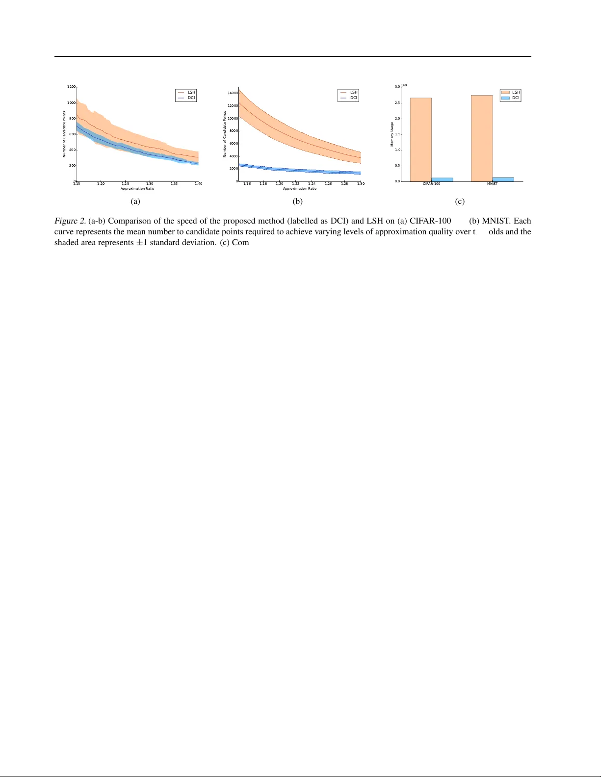
F ast k -Near est Neighbour Search via Dynamic Continuous Indexing Ke Li K E . L I @ E E C S . B E R K E L E Y . E D U Jitendra Malik M A L I K @ E E C S . B E R K E L E Y . E D U Univ ersity of California, Berkele y , CA 94720, United States Abstract Existing methods for retrie ving k -nearest neigh- bours suffer from the curse of dimensionality . W e argue this is caused in part by inherent de- ficiencies of space partitioning, which is the un- derlying strate gy used by most existing methods. W e de vise a ne w strate gy that a voids partitioning the vector space and present a nov el randomized algorithm that runs in time linear in dimensional- ity of the space and sub-linear in the intrinsic di- mensionality and the size of the dataset and tak es space constant in dimensionality of the space and linear in the size of the dataset. The proposed algorithm allo ws fine-grained control o ver accu- racy and speed on a per-query basis, automati- cally adapts to variations in data density , supports dynamic updates to the dataset and is easy-to- implement. W e show appealing theoretical prop- erties and demonstrate empirically that the pro- posed algorithm outperforms locality-sensiti vity hashing (LSH) in terms of approximation quality , speed and space efficienc y . 1. Introduction The k -nearest neighbour method is commonly used both as a classifier and as subroutines in more complex algorithms in a wide range domains, including machine learning, com- puter vision, graphics and robotics. Consequently , finding a fast algorithm for retrieving nearest neighbours has been a subject of sustained interest among the artificial intelli- gence and the theoretical computer science communities alike. W ork over the past several decades has produced a rich collection of algorithms; howe ver , they suffer from one key shortcoming: as the ambient or intrinsic dimen- Pr oceedings of the 33 rd International Conference on Machine Learning , New Y ork, NY , USA, 2016. JMLR: W&CP v olume 48. Copyright 2016 by the author(s). sionality 1 increases, the running time and/or space com- plexity grows rapidly; this phenomenon is often kno wn as the curse of dimensionality . Finding a solution to this prob- lem has pro ven to be elusiv e and has been conjectured to be fundamentally impossible ( Minsky & Seymour , 1969 ). In this era of rapid growth in both the v olume and dimension- ality of data, it has become increasingly important to de vise a fast algorithm that scales to high dimensional space. W e argue that the dif ficulty in ov ercoming the curse of di- mensionality stems in part from inherent deficiencies in space partitioning, the strategy that underlies most exist- ing algorithms. Space partitioning is a divide-and-conquer strategy that partitions the v ector space into a finite number of cells and keeps track of the data points that each cell con- tains. At query time, exhaustiv e search is performed over all data points that lie in cells containing the query point. This strategy forms the basis of most existing algorithms, including k -d trees ( Bentley , 1975 ) and locality-sensitiv e hashing (LSH) ( Indyk & Motwani , 1998 ). While this strategy seems natural and sensible, it suffers from critical deficiencies as the dimensionality increases. Because the volume of any region in the vector space grows exponentially in the dimensionality , either the number or the size of cells must increase exponentially in the number of dimensions, which tends to lead to e xponential time or space comple xity in the dimensionality . In addition, space partitioning limits the algorithm’ s “field of view” to the cell containing the query point; points that lie in adjacent cells hav e no hope of being retrie ved. Consequently , if a query point falls near cell boundaries, the algorithm will fail to retriev e nearby points that lie in adjacent cells. Since the number of such cells is e xponential in the dimensionality , it is intractable to search these cells when dimensionality is high. One popular approach used by LSH and spill trees ( Liu et al. , 2004 ) to mitigate this ef fect is to partition the space using ov erlapping cells and search o ver all points that lie in any of the cells that contain the query point. Because 1 W e use ambient dimensionality to refer to the original dimen- sionality of the space containing the data in order to dif ferentiate it from intrinsic dimensionality , which measures density of the dataset and will be defined precisely later . Fast k -Nearest Neighbour Sear ch via Dynamic Continuous Indexing the ratio of surface area to volume grows in dimension- ality , the number of ov erlapping cells that must be used increases in dimensionality; as a result, the running time or space usage becomes prohibiti vely expensiv e as dimen- sionality increases. Further complications arise from vari- ations in data density across different regions of the space. If the partitioning is too fine, most cells in sparse regions of the space will be empty and so for a query point that lies in a sparse re gion, no points will be retrie ved. If the partitioning is too coarse, each cell in dense regions of the space will contain many points and so for a query point that lies in a dense re gion, many points that are not the true nearest neighbours must be searched. This phenomenon is notably exhibited by LSH, whose performance is highly sensitiv e to the choice of the hash function, which essen- tially defines an implicit partitioning. A good partitioning scheme must therefore depend on the data; howe ver , such data-dependent partitioning schemes would require possi- bly expensi ve preprocessing and prohibit online updates to the dataset. These fundamental limitations of space parti- tioning beg an interesting question: is it possible to de vise a strategy that does not partition the space, yet still enables fast retrie val of nearest neighbours? In this paper , we present a new strate gy for retrie ving k -nearest neighbours that a voids discretizing the vector space, which we call dynamic continuous indexing (DCI). Instead of partitioning the space into discrete cells, we con- struct continuous indices, each of which imposes an order- ing on data points such that closeness in position serves as an approximate indicator of proximity in the vector space. The resulting algorithm runs in time linear in ambient di- mensionality and sub-linear in intrinsic dimensionality and the size of the dataset, while only requiring space con- stant in ambient dimensionality and linear in the size of the dataset. Unlike existing methods, the algorithm allows fine-grained control over accurac y and speed at query time and adapts to varying data density on-the-fly while permit- ting dynamic updates to the dataset. Furthermore, the algo- rithm is easy-to-implement and does not rely on any com- plex or specialized data structure. 2. Related W ork Extensiv e work ov er the past se veral decades has produced a rich collection of algorithms for fast retriev al of k -nearest neighbours. Space partitioning forms the basis of the ma- jority of these algorithms. Early approaches store points in deterministic tree-based data structures, such as k -d trees ( Bentle y , 1975 ), R-trees ( Guttman , 1984 ) and X-trees ( Berchtold et al. , 1996 ; 1998 ), which effecti vely partition the vector space into a hierarchy of half-spaces, hyper- rectangles or V oronoi polygons. These methods achiev e query times that are logarithmic in the number of data points and work very well for low-dimensional data. Un- fortunately , their query times grow exponentially in ambi- ent dimensionality because the number of lea ves in the tree that need to be searched increases exponentially in ambi- ent dimensionality; as a result, for high-dimensional data, these algorithms become slower than exhausti ve search. More recent methods like spill trees ( Liu et al. , 2004 ), RP trees ( Dasgupta & Freund , 2008 ) and virtual spill trees ( Dasgupta & Sinha , 2015 ) extend these approaches by randomizing the dividing hyperplane at each node. Un- fortunately , the number of points in the leaves increases exponentially in the intrinsic dimensionality of the dataset. In an effor t to tame the curse of dimensionality , re- searchers hav e considered relaxing the problem to allow  - approximate solutions, which can contain any point whose distance to the query point differs from that of the true nearest neighbours by at most a factor of (1 +  ) . T ree- based methods ( Arya et al. , 1998 ) hav e been proposed for this setting; unfortunately , the running time still exhibits exponential dependence on dimensionality . Another pop- ular method is locality-sensitiv e hashing (LSH) ( Indyk & Motwani , 1998 ; Datar et al. , 2004 ), which relies on a hash function that implicitly defines a partitioning of the space. Unfortunately , LSH struggles on datasets with v arying den- sity , as cells in sparse regions of the space tend to be empty and cells in dense regions tend to contain a large number of points. As a result, it fails to return any point on some queries and requires a long time on some others. This moti- vated the de velopment of data-dependent hashing schemes based on k -means ( Paule v ´ e et al. , 2010 ) and spectral parti- tioning ( W eiss et al. , 2009 ). Unfortunately , these methods do not support dynamic updates to the dataset or provide correctness guarantees. Furthermore, they incur a signifi- cant pre-processing cost, which can be expensiv e on large datasets. Other data-dependent algorithms outside the LSH framew ork have also been proposed, such as ( Fukunaga & Narendra , 1975 ; Brin , 1995 ; Nister & Stewenius , 2006 ; W ang , 2011 ), which work by constructing a hierarchy of clusters using k -means and can be viewed as performing a highly data-dependent form of space partitioning. For these algorithms, no guarantees on approximation quality or running time are known. One class of methods ( Orchard , 1991 ; Arya & Mount , 1993 ; Clarkson , 1999 ; Karger & Ruhl , 2002 ) that does not rely on space partitioning uses a local search strategy . Start- ing from a random data point, these methods iteratively find a new data point that is closer to the query than the previ- ous data point. Unfortunately , the performance of these methods deteriorates in the presence of significant varia- tions in data density , since it may take v ery long to navigate a dense region of the space, even if it is very far from the query . Other methods like navigating nets ( Krauthgamer & Lee , 2004 ), co ver tree s ( Beygelzimer et al. , 2006 ) and rank Fast k -Nearest Neighbour Sear ch via Dynamic Continuous Indexing cov er trees ( Houle & Nett , 2015 ) adopt a coarse-to-fine strategy . These methods work by maintaining coarse sub- sets of points at varying scales and progressi vely searching the neighbourhood of the query with decreasing radii at in- creasingly finer scales. Sadly , the running times of these methods again exhibit exponential dependence on the in- trinsic dimensionality . W e direct interested readers to ( Clarkson , 2006 ) for a com- prehensiv e survey of existing methods. 3. Algorithm Algorithm 1 Algorithm for data structure construction Require: A dataset D of n points p 1 , . . . , p n , the number of sim- ple indices m that constitute a composite index and the number of composite indices L function C O N S T RU C T ( D, m, L ) { u j l } j ∈ [ m ] ,l ∈ [ L ] ← mL random unit vectors in R d { T j l } j ∈ [ m ] ,l ∈ [ L ] ← mL empty binary search trees or skip lists for j = 1 to m do for l = 1 to L do for i = 1 to n do p i j l ← h p i , u j l i Insert ( p i j l , i ) into T j l with p i j l being the key and i being the value end for end for end for retur n { ( T j l , u j l ) } j ∈ [ m ] ,l ∈ [ L ] end function The proposed algorithm relies on the construction of continuous indices of data points that support both fast searching and online updates. T o this end, we use one- dimensional random projections as basic building blocks and construct mL simple indices, each of which orders data points by their projections along a random direction. Such an index has both desired properties: data points can be efficiently retrieved and updated when the index is imple- mented using standard data structures for storing ordered sequences of scalars, like self-balancing binary search trees or skip lists. This ordered arrangement of data points ex- ploits an important property of the k -nearest neighbour search problem that has often been overlook ed: it suffices to construct an index that approximately preserves the rel- ativ e or der between the true k -nearest neighbours and the other data points in terms of their distances to the query point without necessarily preserving all pairwise distances. This observation enables projection to a much lower di- mensional space than the Johnson-Lindenstrauss transform ( Johnson & Lindenstrauss , 1984 ). W e show in the follow- ing section that with high probability , one-dimensional ran- dom projection preserves the relativ e order of two points whose distances to the query point differ significantly re- gardless of the ambient dimensionality of the points. Algorithm 2 Algorithm for k -nearest neighbour retrie val Require: Query point q in R d , binary search trees/skip lists and their associated projection vectors { ( T j l , u j l ) } j ∈ [ m ] ,l ∈ [ L ] , and maximum tolerable failure probability  function Q U E RY ( q , { ( T j l , u j l ) } j,l ,  ) C l ← array of size n with entries initialized to 0 ∀ l ∈ [ L ] q j l ← h q , u j l i ∀ j ∈ [ m ] , l ∈ [ L ] S l ← ∅ ∀ l ∈ [ L ] for i = 1 to n do for l = 1 to L do for j = 1 to m do ( p ( i ) j l , h ( i ) j l ) ← the node in T j l whose key is the i th closest to q j l C l [ h ( i ) j l ] ← C l [ h ( i ) j l ] + 1 end for for j = 1 to m do if C l [ h ( i ) j l ] = m then S l ← S l ∪ { h ( i ) j l } end if end for end for if IsStoppingConditionSatisfied ( i, S l ,  ) then break end if end for retur n k points in S l ∈ [ L ] S l that are the closest in Euclidean distance in R d to q end function W e combine each set of m simple indices to form a com- posite index in which points are ordered by the maximum difference ov er all simple indices between the positions of the point and the query in the simple index. The compos- ite index enables fast retriev al of a small number of data points, which will be referred to as candidate points, that are close to the query point along se veral random directions and therefore are likely to be truly close to the query . The composite indices are not explicitly constructed; instead, each of them simply keeps track of the number of its con- stituent simple indices that hav e encountered any particular point and returns a point as soon as all its constituent simple indices hav e encountered that point. At query time, we retriev e candidate points from each com- posite index one by one in the order they are returned until some stopping condition is satisfied, while omitting points that hav e been previously retriev ed from other composite indices. Exhaustive search is then performed over candi- date points retriev ed from all L composite indices to iden- tify the subset of k points closest to the query . Please refer to Algorithms 1 and 2 for a precise statement of the con- struction and querying procedures. Because data points are retriev ed according to their posi- tions in the composite index rather than the regions of space Fast k -Nearest Neighbour Sear ch via Dynamic Continuous Indexing v s Pr    h v l ,u i      h v s ,u i    h v s ,u i h v l ,u i v l (a) v l v s U ( v s ,v l ) (b) v s v l 1 v l 2 U ( v s ,v l 1 ) \ U ( v s ,v l 2 ) (c) Figure 1. (a) Examples of order-preserving (sho wn in green) and order-in verting (shown in red) projection directions. Any projection direction within the shaded region in verts the relativ e order of the vectors by length under projection, while any projection directions outside the region preserves it. The size of the shaded region depends on the ratio of the lengths of the vectors. (b) Projection vectors whose endpoints lie in the shaded region would be order-in verting. (c) Projection v ectors whose endpoints lie in the shaded re gion would in vert the order of both long v ectors relativ e to the short vector . Best viewed in colour . they lie in, the algorithm is able to automatically adapt to changes in data density as dynamic updates are made to the dataset without requiring any pre-processing to esti- mate data density at construction time. Also, unlike ex- isting methods, the number of retrieved candidate points can be controlled on a per-query basis, enabling the user to easily trade off accuracy against speed. W e dev elop two versions of the algorithm, a data-independent and a data- dependent version, which differ in the stopping condition that is used. In the former , the number of candidate points is indirectly preset according to the global data density and the maximum tolerable f ailure probability; in the latter , the number of candidate points is chosen adaptiv ely at query time based on the local data density in the neighbourhood of the query . W e analyze the algorithm below and show that its failure probability is independent of ambient dimension- ality , its running time is linear in ambient dimensionality and sub-linear in intrinsic dimensionality and the size of the dataset and its space complexity is independent of am- bient dimensionality and linear in the size of the dataset. 3.1. Properties of Random 1D Pr ojection First, we examine the effect of projecting d -dimensional vectors to one dimension, which motiv ates its use in the proposed algorithm. W e are interested in the probability that a distant point appears closer than a nearby point under projection; if this probability is low , then each simple index approximately preserves the order of points by distance to the query point. If we consider displacement vectors be- tween the query point and data points, this probability is then is equiv alent to the probability of the lengths of these vectors in verting under projection. Lemma 1. Let v l , v s ∈ R d such that   v l   2 >   v s   2 , and u ∈ R d be a unit vector drawn uniformly at random. Then the pr obability of v s being at least as long as v l under pr ojection u is at most 1 − 2 π cos − 1    v s   2 /   v l   2  . Pr oof. Assuming that v l and v s are not collinear, consider the two-dimensional subspace spanned by v l and v s , which we will denote as P . (If v l and v s are collinear , we define P to be the subspace spanned by v l and an arbitrary vector that’ s linearly independent of v l .) For any vector w , we use w k and w ⊥ to denote the components of w in P and P ⊥ such that w = w k + w ⊥ . For w ∈ { v s , v l } , because w ⊥ = 0 , h w , u i = h w , u k i . So, we can limit our attention to P for this analysis. W e parameterize u k in terms of its angle relati ve to v l , which we denote as θ . Also, we denote the angle of u k relativ e to v s as ψ . Then, Pr     h v l , u i    ≤    h v s , u i     = Pr     h v l , u k i    ≤    h v s , u k i     = Pr     v l    2    u k    2 | cos θ | ≤    v s    2    u k    2 | cos ψ |  ≤ Pr  | cos θ | ≤ k v s k 2 k v l k 2  = 2Pr  θ ∈  cos − 1  k v s k 2 k v l k 2  , π − cos − 1  k v s k 2 k v l k 2  = 1 − 2 π cos − 1  k v s k 2 k v l k 2  Observe that if   h v l , u i   ≤   h v s , u i   , the relative order of v l and v s by their lengths would be inv erted when projected along u . This occurs when u k is close to orthogonal to v l , which is illustrated in Figure 1a . Also note that the probability of in verting the relativ e order of v l and v s is small when v l is much longer than v s . On the other hand, Fast k -Nearest Neighbour Sear ch via Dynamic Continuous Indexing this probability is high when v l and v s are similar in length, which corresponds to the case when two data points are almost equidistant to the query point. So, if we consider a sequence of vectors ordered by length, applying random one-dimensional projection will likely perturb the ordering locally , but will preserve the ordering globally . Next, we build on this result to analyze the order-in version probability when there are more than two vectors. Consider the sample space B =  u ∈ R d   k u k 2 = 1  and the set U ( v s , v l ) =  u ∈ B   | cos θ | ≤   v s   2 /   v l   2  , which is illustrated in Figure 1b , where θ is the angle between u k and v l . If we use area ( U ) to denote the area of the region formed by the endpoints of all vectors in the set U , then we can rewrite the above bound on the order-in version proba- bility as: Pr     h v l , u i    ≤    h v s , u i     ≤ Pr  u ∈ U ( v s , v l )  = area ( V s l ) area ( B ) = 1 − 2 π cos − 1  k v s k 2 k v l k 2  Lemma 2. Let  v l i  N i =1 be a set of vectors such that   v l i   2 >   v s   2 ∀ i ∈ [ N ] . Then the pr obabil- ity that there is a subset of k 0 vectors fr om  v l i  N i =1 that are all not longer than v s under pr ojection is at most 1 k 0 P N i =1  1 − 2 π cos − 1    v s   2 /   v l i   2  . Fur- thermor e, if k 0 = N , this pr obability is at most min i ∈ [ N ]  1 − 2 π cos − 1    v s   2 /   v l i   2  . Pr oof. For a giv en subset I ⊆ [ N ] of size k 0 , the probability that all vectors indexed by ele- ments in I are not longer than v s under pro- jection u is at most Pr  u ∈ T i ∈ I U ( v s , v l i )  = area  T i ∈ I U ( v s , v l i )  / area ( B ) . So, the prob- ability that this occurs on some subset I is at most Pr  u ∈ S I ⊆ [ N ]: | I | = k 0 T i ∈ I U ( v s , v l i )  = area  S I ⊆ [ N ]: | I | = k 0 T i ∈ I U ( v s , v l i )  / area ( B ) . Observe that each point in S I ⊆ [ N ]: | I | = k 0 T i ∈ I U ( v s , v l i ) must be cov ered by at least k 0 U ( v s , v l i ) ’ s. So, k 0 · area   [ I ⊆ [ N ]: | I | = k 0 \ i ∈ I U ( v s , v l i )   ≤ N X i =1 area  U ( v s , v l i )  It follows that the probability this ev ent occurs on some subset I is bounded above by 1 k 0 P N i =1 area ( U ( v s ,v l i ) ) area ( B ) = 1 k 0 P N i =1  1 − 2 π cos − 1    v s   2 /   v l i   2  . If k 0 = N , we use the fact that area  T i ∈ [ N ] U ( v s , v l i )  ≤ min i ∈ [ N ]  area  U ( v s , v l i )  to obtain the desired re- sult. Intuitiv ely , if this ev ent occurs, then there are at least k 0 vectors that rank abov e v s when sorted in nondecreasing order by their lengths under projection. This can only oc- cur when the endpoint of u falls in a region on the unit sphere corresponding to S I ⊆ [ N ]: | I | = k 0 T i ∈ I U ( v s , v l i ) . W e illustrate this region in Figure 1c for the case of d = 3 . Theorem 3. Let  v l i  N i =1 and  v s i 0  N 0 i 0 =1 be sets of vectors such that   v l i   2 > k v s i 0 k 2 ∀ i ∈ [ N ] , i 0 ∈ [ N 0 ] . Then the pr obability that there is a subset of k 0 vectors fr om  v l i  N i =1 that ar e all not longer than some v s i 0 under pr ojection is at most 1 k 0 P N i =1  1 − 2 π cos − 1    v s max   2 /   v l i   2  , wher e   v s max   2 ≥ k v s i 0 k 2 ∀ i 0 ∈ [ N 0 ] . Pr oof. The probability that this ev ent occurs is at most Pr  u ∈ S i 0 ∈ [ N 0 ] S I ⊆ [ N ]: | I | = k 0 T i ∈ I U ( v s i 0 , v l i )  . W e observe that for all i, i 0 ,  θ   | cos θ | ≤ k v s i 0 k 2 /   v l i   2  ⊆  θ   | cos θ | ≤   v s max   2 /   v l i   2  , which implies that U ( v s i 0 , v l i ) ⊆ U ( v s max , v l i ) . If we take the intersection followed by union on both sides, we obtain S I ⊆ [ N ]: | I | = k 0 T i ∈ I U ( v s i 0 , v l i ) ⊆ S I ⊆ [ N ]: | I | = k 0 T i ∈ I U ( v s max , v l i ) . Because this is true for all i 0 , S i 0 ∈ [ N 0 ] S I ⊆ [ N ]: | I | = k 0 T i ∈ I U ( v s i 0 , v l i ) ⊆ S I ⊆ [ N ]: | I | = k 0 T i ∈ I U ( v s max , v l i ) . Therefore, this probability is bounded above by Pr  u ∈ S I ⊆ [ N ]: | I | = k 0 T i ∈ I U ( v s max , v l i )  . By Lemma 2 , this is at most 1 k 0 P N i =1  1 − 2 π cos − 1    v s max   2 /   v l i   2  . 3.2. Data Density W e now formally characterize data density by defining the following notion of local relati ve sparsity: Definition 4. Given a dataset D ⊆ R d , let B p ( r ) be the set of points in D that are within a ball of radius r around a point p . W e say D has local r elative sparsity of ( τ , γ ) at a point p ∈ R d if for all r suc h that | B p ( r ) | ≥ τ , | B p ( γ r ) | ≤ 2 | B p ( r ) | , wher e γ ≥ 1 . Intuitiv ely , γ represents a lower bound on the increase in ra- dius when the number of points within the ball is doubled. When γ is close to 1 , the dataset is dense in the neighbour - hood of p , since there could be many points in D that are al- most equidistant from p . Retrieving the nearest neighbours of such a p is considered “hard”, since it would be dif ficult to tell which of these points are the true nearest neighbours without computing the distances to all these points exactly . Fast k -Nearest Neighbour Sear ch via Dynamic Continuous Indexing W e also define a related notion of global relativ e sparsity , which we will use to derive the number of iterations the outer loop of the querying function should be executed and a bound on the running time that is independent of the query: Definition 5. A dataset D has global r elative sparsity of ( τ , γ ) if for all r and p ∈ R d such that | B p ( r ) | ≥ τ , | B p ( γ r ) | ≤ 2 | B p ( r ) | , wher e γ ≥ 1 . Note that a dataset with global relativ e sparsity of ( τ , γ ) has local relativ e sparsity of ( τ , γ ) at ev ery point. Global relativ e sparsity is closely related to the notion of expan- sion rate introduced by ( Karger & Ruhl , 2002 ). More specifically , a dataset with global relative sparsity of ( τ , γ ) has ( τ , 2 (1 / log 2 γ ) ) -expansion, where the latter quantity is known as the expansion rate. If we use c to denote the ex- pansion rate, the quantity log 2 c is known as the intrinsic dimension ( Clarkson , 2006 ), since when the dataset is uni- formly distributed, intrinsic dimensionality would match ambient dimensionality . So, the intrinsic dimension of a dataset with global relativ e sparsity of ( τ , γ ) is 1 / log 2 γ . 3.3. Data-Independent V ersion In the data-independent version of the algorithm, the outer loop in the querying function executes for a preset number of iterations ˜ k . The values of L , m and ˜ k are fixed for all queries and will be chosen later . W e apply the results obtained above to analyze the algo- rithm. Consider the event that the algorithm fails to return the correct set of k -nearest neighbours – this can only oc- cur if a true k -nearest neighbour is not contained in any of the S l ’ s, which entails that for each l ∈ [ L ] , there is a set of ˜ k − k + 1 points that are not the true k -nearest neighbours but are closer to the query than the true k -nearest neigh- bours under some of the projections u 1 l , . . . , u ml . W e an- alyze the probability that this occurs below and deriv e the parameter settings that ensure the algorithm succeeds with high probability . Please refer to the supplementary material for proofs of the following results. Lemma 6. F or a dataset with global r el- ative spar sity ( k, γ ) , ther e is some ˜ k ∈ Ω(max( k log( n/k ) , k ( n/k ) 1 − log 2 γ )) such that the pr obability that the candidate points r etrieved fr om a given composite index do not include some of the true k -near est neighbours is at most some constant α < 1 . Theorem 7. F or a dataset with global r elative spar- sity ( k , γ ) , for any  > 0 , ther e is some L and ˜ k ∈ Ω(max( k log( n/k ) , k ( n/k ) 1 − log 2 γ )) such that the algo- rithm returns the correct set of k -near est neighbours with pr obability of at least 1 −  . The abov e result suggests that we should choose ˜ k ∈ Ω(max( k log( n/k ) , k ( n/k ) 1 − log 2 γ )) to ensure the algo- rithm succeeds with high probability . Next, we analyze the time and space complexity of the algorithm. Proofs of the following results are found in the supplementary material. Theorem 8. The algorithm takes O (max( dk log ( n/k ) , dk ( n/k ) 1 − 1 /d 0 )) time to r etrieve the k -near est neighbours at query time, where d 0 denotes the intrinsic dimension of the dataset. Theorem 9. The algorithm takes O ( dn + n log n ) time to pr eprocess the data points in D at construction time. Theorem 10. The algorithm r equires O ( d + log n ) time to insert a new data point and O (log n ) time to delete a data point. Theorem 11. The algorithm requir es O ( n ) space in addi- tion to the space used to stor e the data. 3.4. Data-Dependent V ersion Conceptually , performance of the proposed algorithm de- pends on two factors: how likely the index returns the true nearest neighbours before other points and when the algo- rithm stops retrieving points from the inde x. The preceding sections primarily focused on the former; in this section, we take a closer look at the latter . One strategy , which is used by the data-independent ver - sion of the algorithm, is to stop after a preset number of it- erations of the outer loop. Although simple, such a strategy leav es much to be desired. First of all, in order to set the number of iterations, it requires knowledge of the global relativ e sparsity of the dataset, which is rarely known a pri- ori. Computing this is either very expensi ve in the case of datasets or infeasible in the case of streaming data, as global relativ e sparsity may change as new data points ar- riv e. More importantly , it is unable to tak e adv antage of the local relati ve sparsity in the neighbourhood of the query . A method that is capable of adapting to local relati ve sparsity could potentially be much faster because query points tend to be close to the manifold on which points in the dataset lie, resulting in the dataset being sparse in the neighbour- hood of the query point. Ideally , the algorithm should stop as soon as it has re- triev ed the true nearest neighbours. Determining if this is the case amounts to asking if there exists a point that we hav e not seen lying closer to the query than the points we hav e seen. At first sight, because nothing is known about unseen points, it seems not possible to do better than ex- haustiv e search, as we can only rule out the existence of such a point after computing distances to all unseen points. Somewhat surprisingly , by exploiting the fact that the pro- jections associated with the index are random, it is possible to make inferences about points that we hav e nev er seen. W e do so by lev eraging ideas from statistical hypothesis testing. Fast k -Nearest Neighbour Sear ch via Dynamic Continuous Indexing After each iteration of the outer loop, we perform a hypoth- esis test, with the null hypothesis being that the complete set of the k -nearest neighbours has not yet been retrieved. Rejecting the null hypothesis implies accepting the alterna- tiv e hypothesis that all the true k -nearest neighbours have been retriev ed. At this point, the algorithm can safely ter- minate while guaranteeing that the probability that the al- gorithm fails to return the correct results is bounded above by the significance lev el. The test statistic is an upper bound on the probability of missing a true k -nearest neigh- bour . The resulting algorithm does not require any prior knowledge about the dataset and terminates earlier when the dataset is sparse in the neighbourhood of the query; for this reason, we will refer to this version of the algorithm as the data-dependent version. More concretely , as the algorithm retriev es candidate points, it computes their true distances to the query and maintains a list of k points that are the closest to the query among the points retriev ed from all composite in- dices so far . Let ˜ p ( i ) and ˜ p max l denote the i th closest candidate point to q retrieved from all composite indices and the farthest candidate point from q retriev ed from the l th composite index respectively . When the number of candidate points e xceeds k , the algorithm checks if Q L l =1  1 −  2 π cos − 1    ˜ p ( k ) − q   2 /   ˜ p max l − q   2  m  ≤  , where  is the maximum tolerable failure probability , af- ter each iteration of the outer loop. If the condition is satis- fied, the algorithm terminates and returns  ˜ p ( i )  k i =1 . W e sho w the correctness and running time of this algorithm below . Proofs of the follo wing results are found in the sup- plementary material. Theorem 12. F or any  > 0 , m and L , the data-dependent algorithm r eturns the correct set of k -near est neighbours of the query q with probability of at least 1 −  . Theorem 13. On a dataset with global r el- ative spar sity ( k , γ ) , given fixed parameters m and L , the data-dependent algorithm takes O max dk log  n k  , dk  n k  1 − 1 /d 0 , d  1 − m √ 1 − L √   d 0 !! time with high pr obability to r etrieve the k -nearest neighbours at query time, where d 0 denotes the intrinsic dimension of the dataset. Note that we can make the denominator of the last argu- ment arbitrarily close to 1 by choosing a lar ge L . 4. Experiments W e compare the performance of the proposed algorithm to that of LSH, which is arguably the most popular method for fast nearest neighbour retriev al. Because LSH is designed for the approximate setting, under which the performance metric of interest is ho w close the points returned by the al- gorithm are to the query rather than whether the returned points are the true k -nearest neighbours, we empirically ev aluate performance in this setting. Because the distance metric of interest is the Euclidean distance, we compare to Exact Euclidean LSH ( E 2 LSH ) ( Datar et al. , 2004 ), which uses hash functions designed for Euclidean space. W e compare the performance of the proposed algorithm and LSH on the CIF AR-100 and MNIST datasets, which consist of 32 × 32 colour images of various real-w orld ob- jects and 28 × 28 grayscale images of handwritten digits respectiv ely . W e reshape the images into v ectors, with each dimension representing the pixel intensity at a particular lo- cation and colour channel of the image. The resulting vec- tors have a dimensionality of 32 × 32 × 3 = 3072 in the case of CIF AR-100 and 28 × 28 = 784 in the case of MNIST , so the dimensionality under consideration is higher than what traditional tree-based algorithms can handle. W e combine the training set and the test set of each dataset, and so we hav e a total of 60 , 000 instances in CIF AR-100 and 70 , 000 instances in MNIST . W e randomize the instances that serve as queries using cross-validation. Specifically , we randomly select 100 in- stances to serve as query points and the designate the re- maining instances as data points. Each algorithm is then used to retrieve approximate k -nearest neighbours of each query point among the set of all data points. This procedure is repeated for ten folds, each with a different split of query vs. data points. W e compare the number of candidate points that each algo- rithm requires to achieve a desired lev el of approximation quality . W e quantify approximation quality using the ap- proximation ratio, which is defined as the ratio of the radius of the ball containing approximate k -nearest neighbours to the radius of the ball containing true k -nearest neighbours. So, the smaller the approximation ratio, the better the ap- proximation quality . Because dimensionality is high and exhausti ve search must be performed over all candidate points, the time taken for compute distances between the candidate points and the query dominates the ov erall run- ning time of the querying operation. Therefore, the number of candidate points can be viewed as an implementation- independent proxy for the running time. Because the hash table constructed by LSH depends on the desired le vel of approximation quality , we construct a dif- ferent hash table for each lev el of approximation quality . On the other hand, the indices constructed by the proposed method are not specific to any particular lev el of approxi- mation quality; instead, approximation quality can be con- trolled at query time by v arying the number of iterations of the outer loop. So, the same indices are used for all levels of approximation quality . Therefore, our ev aluation scheme is Fast k -Nearest Neighbour Sear ch via Dynamic Continuous Indexing 1.15 1.20 1.25 1.30 1.35 1.40 Approximation Ratio 0 200 400 600 800 1000 1200 Number of Candidate Points LSH DCI (a) 1.16 1.18 1.20 1.22 1.24 1.26 1.28 1.30 Approximation Ratio 0 2000 4000 6000 8000 10000 12000 14000 Number of Candidate Points LSH DCI (b) CIFAR-100 MNIST 0.0 0.5 1.0 1.5 2.0 2.5 3.0 Memory Usage 1e8 LSH DCI (c) Figure 2. (a-b) Comparison of the speed of the proposed method (labelled as DCI) and LSH on (a) CIF AR-100 and (b) MNIST . Each curve represents the mean number to candidate points required to achie ve v arying levels of approximation quality over ten folds and the shaded area represents ± 1 standard de viation. (c) Comparison of the space efficienc y of the proposed method and LSH on CIF AR-100 and MNIST . The height of each bar represents the a verage amount of memory used by each method to achie ve the performance shown in (a) and (b). biased tow ards LSH and against the proposed method. W e adopt the recommended guidelines for choosing param- eters of LSH and used 24 hashes per table and 100 tables. For the proposed method, we used m = 25 and L = 2 on CIF AR-100 and m = 15 and L = 3 on MNIST , which we found to work well in practice. In Figures 2a and 2b , we plot the performance of the proposed method and LSH on the CIF AR-100 and MNIST datasets for retrieving 25 - nearest neighbours. For the purposes of retrieving nearest neighbours, MNIST is a more challenging dataset than CIF AR-100. This is be- cause the instances in MNIST form dense clusters, whereas the instances in CIF AR-100 are more visually diverse and so are more dispersed in space. Intuitiv ely , if the query falls inside a dense cluster of points, there are many points that are very close to the query and so it is difficult to distinguish true nearest neighbours from points that are only slightly farther a way . V iewed differently , because true nearest neighbours tend to be extremely close to the query on MNIST , the denominator for computing the approxima- tion ratio is usually very small. Consequently , returning points that are only slightly f arther a way than the true near- est neighbours would result in a large approximation ratio. As a result, both the proposed method and LSH require far more candidate points on MNIST than on CIF AR-100 to achiev e comparable approximation ratios. W e find the proposed method achiev es better performance than LSH at all lev els of approximation quality . Notably , the performance of LSH degrades drastically on MNIST , which is not surprising since LSH is known to have difficul- ties on datasets with lar ge v ariations in data density . On the other hand, the proposed method requires 61 . 3% − 78 . 7% fewer candidate points than LSH to achiev e the same ap- proximation quality while using less than 1 / 20 of the mem- ory . 5. Conclusion In this paper , we delineated the inherent deficiencies of space partitioning and presented a ne w strategy for fast retriev al of k -nearest neighbours, which we dub dynamic continuous inde xing (DCI). Instead of discretizing the vec- tor space, the proposed algorithm constructs continuous in- dices, each of which imposes an ordering of data points in which closeby positions approximately reflect proximity in the vector space. Unlike existing methods, the proposed algorithm allows granular control over accuracy and speed on a per-query basis, adapts to variations to data density on-the-fly and supports online updates to the dataset. W e analyzed the proposed algorithm and sho wed it runs in time linear in ambient dimensionality and sub-linear in intrinsic dimensionality and the size of the dataset and takes space constant in ambient dimensionality and linear in the size of the dataset. Furthermore, we demonstrated empirically that the proposed algorithm compares fa vourably to LSH in terms of approximation quality , speed and space efficienc y . Acknowledgements. Ke Li thanks the Berkeley V ision and Learning Center (BVLC) and the Natural Sciences and Engineering Research Council of Canada (NSERC) for fi- nancial support. The authors also thank Lap Chi Lau and the anonymous re viewers for feedback. References Arya, Sunil and Mount, David M. Approximate nearest neighbor queries in fixed dimensions. In SOD A , vol- ume 93, pp. 271–280, 1993. Fast k -Nearest Neighbour Sear ch via Dynamic Continuous Indexing Arya, Sunil, Mount, David M, Netanyahu, Nathan S, Sil- verman, Ruth, and W u, Angela Y . An optimal algo- rithm for approximate nearest neighbor searching fixed dimensions. J ournal of the ACM (JA CM) , 45(6):891– 923, 1998. Bentley , Jon Louis. Multidimensional binary search trees used for associativ e searching. Communications of the A CM , 18(9):509–517, 1975. Berchtold, Stefan, Keim, Daniel A., and peter Kriegel, Hans. The X-tree : An Index Structure for High- Dimensional Data. In V ery Large Data Bases , pp. 28–39, 1996. Berchtold, Stefan, Ertl, Bernhard, Keim, Daniel A, Kriegel, H-P , and Seidl, Thomas. Fast nearest neighbor search in high-dimensional space. In Data Engineering, 1998. Pr oceedings., 14th International Confer ence on , pp. 209–218. IEEE, 1998. Beygelzimer , Alina, Kakade, Sham, and Langford, John. Cov er trees for nearest neighbor . In Pr oceedings of the 23r d international confer ence on Machine learning , pp. 97–104. A CM, 2006. Brin, Sergey . Near neighbor search in large metric spaces. VLDB , pp. 574584, 1995. Clarkson, Kenneth L. Nearest neighbor queries in metric spaces. Discrete & Computational Geometry , 22(1):63– 93, 1999. Clarkson, Kenneth L. Nearest-neighbor searching and met- ric space dimensions. Near est-neighbor methods for learning and vision: theory and practice , pp. 15–59, 2006. Dasgupta, Sanjoy and Freund, Y oav . Random projection trees and low dimensional manifolds. In Pr oceedings of the fortieth annual ACM symposium on Theory of com- puting , pp. 537–546. A CM, 2008. Dasgupta, Sanjoy and Sinha, Kaushik. Randomized parti- tion trees for nearest neighbor search. Algorithmica , 72 (1):237–263, 2015. Datar , Mayur , Immorlica, Nicole, Indyk, Piotr , and Mir- rokni, V ahab S. Locality-sensitive hashing scheme based on p-stable distributions. In Pr oceedings of the twenti- eth annual symposium on Computational geometry , pp. 253–262. A CM, 2004. Fukunaga, Keinosuke and Narendra, Patrenahalli M. A branch and bound algorithm for computing k-nearest neighbors. Computers, IEEE T ransactions on , 100(7): 750–753, 1975. Guttman, Antonin. R-tr ees: a dynamic index structure for spatial sear ching , volume 14. A CM, 1984. Houle, Michael E and Nett, Michael. Rank-based similarity search: Reducing the dimensional dependence. P attern Analysis and Machine Intelligence, IEEE T ransactions on , 37(1):136–150, 2015. Indyk, Piotr and Motwani, Rajeev . Approximate nearest neighbors: towards removing the curse of dimensional- ity . In Pr oceedings of the thirtieth annual ACM sympo- sium on Theory of computing , pp. 604–613. ACM, 1998. Johnson, William B and Lindenstrauss, Joram. Extensions of Lipschitz mappings into a Hilbert space. Contempo- rary mathematics , 26(189-206):1, 1984. Karger , David R and Ruhl, Matthias. Finding nearest neighbors in growth-restricted metrics. In Pr oceedings of the thiry-fourth annual A CM symposium on Theory of computing , pp. 741–750. A CM, 2002. Krauthgamer , Robert and Lee, James R. Na vigating nets: simple algorithms for proximity search. In Pr oceedings of the fifteenth annual ACM-SIAM symposium on Dis- cr ete algorithms , pp. 798–807. Society for Industrial and Applied Mathematics, 2004. Liu, T ing, Moore, Andrew W , Y ang, Ke, and Gray , Ale xan- der G. An in vestigation of practical approximate nearest neighbor algorithms. In Advances in Neural Information Pr ocessing Systems , pp. 825–832, 2004. Minsky , Marvin and Seymour , Papert. Perceptrons: an in- troduction to computational geometry . pp. 222, 1969. Nister , David and Stewenius, Henrik. Scalable recognition with a vocabulary tree. In Computer V ision and P attern Recognition, 2006 IEEE Computer Society Confer ence on , volume 2, pp. 2161–2168. IEEE, 2006. Orchard, Michael T . A fast nearest-neighbor search al- gorithm. In Acoustics, Speech, and Signal Pr ocessing, 1991. ICASSP-91., 1991 International Confer ence on , pp. 2297–2300. IEEE, 1991. Paule v ´ e, Lo ¨ ıc, J ´ egou, Herv ´ e, and Amsaleg, Laurent. Lo- cality sensitiv e hashing: A comparison of hash function types and querying mechanisms. P attern Recognition Letters , 31(11):1348–1358, 2010. W ang, Xueyi. A fast exact k-nearest neighbors algorithm for high dimensional search using k-means clustering and triangle inequality . In Neural Networks (IJCNN), The 2011 International Joint Confer ence on , pp. 1293– 1299. IEEE, 2011. W eiss, Y air , T orralba, Antonio, and Fergus, Rob . Spectral hashing. In Advances in Neural Information Processing Systems , pp. 1753–1760, 2009. F ast k -Near est Neighbour Search via Dynamic Continuous Indexing Supplementary Material Ke Li K E . L I @ E E C S . B E R K E L E Y . E D U Jitendra Malik M A L I K @ E E C S . B E R K E L E Y . E D U Univ ersity of California, Berkeley , CA 94720, United States Below , we present proofs of the results sho wn in the paper . W e first prov e two intermediate results, which are used to deriv e results in the paper . Throughout our proofs, we use { p ( i ) } n i =1 to denote a re-ordering of the points { p i } n i =1 so that p ( i ) is the i th closest point to the query q . For any giv en projection direction u j l associated with a simple index, we also consider a ranking of the points { p i } n i =1 by their dis- tance to q under projection u j l in nondecreasing order . W e say points are ranked before others if they appear earlier in this ranking. Lemma 14. The pr obability that for all constituent simple indices of a composite index, fe wer than n 0 points exist that ar e not the true k -nearest neigh- bours b ut are ranked befor e some of them, is at least  1 − 1 n 0 − k P n i =2 k +1 k p ( k ) − q k 2 k p ( i ) − q k 2  m . Pr oof. For any given simple index, we will refer to the points that are not the true k -nearest neighbours but are ranked before some of them as extr aneous points . W e fur- thermore cate gorize the e xtraneous points as either reason- able or silly . An extraneous point is reasonable if it is one of the 2 k -nearest neighbours, and is silly otherwise. Since there can be at most k reasonable extraneous points, there must be at least n 0 − k silly extraneous points. Therefore, the e vent that n 0 extraneous points exist must be contained in the ev ent that n 0 − k silly extraneous points exist. W e find the probability that such a set of silly extraneous points exists for any given simple index. By Theorem 3 , where we take { v s i 0 } N 0 i 0 =1 to be { p ( i ) − q } k i =1 , { v l i } N i =1 to be { p ( i ) − q } n i =2 k +1 and k 0 to be n 0 − k , the probability that there are at least n 0 − k silly extraneous points is at most 1 n 0 − k P n i =2 k +1  1 − 2 π cos − 1  k p ( k ) − q k 2 k p ( i ) − q k 2  . This implies that the probability that at least n 0 extraneous points exist is bounded above by the same quantity , and so the probability that fe wer than n 0 extraneous points exist is at least 1 − 1 n 0 − k P n i =2 k +1  1 − 2 π cos − 1  k p ( k ) − q k 2 k p ( i ) − q k 2  . Hence, the probability that fewer than n 0 ex- traneous points exist for all constituent sim- ples indices of a composite index is at least  1 − 1 n 0 − k P n i =2 k +1  1 − 2 π cos − 1  k p ( k ) − q k 2 k p ( i ) − q k 2  m . Using the fact that 1 − (2 /π ) cos − 1 ( x ) ≤ x ∀ x ∈ [0 , 1] , this quantity is at least  1 − 1 n 0 − k P n i =2 k +1 k p ( k ) − q k 2 k p ( i ) − q k 2  m . Lemma 15. On a dataset with global r elative spar- sity ( k , γ ) , the pr obability that for all constituent simple indices of a composite index, fe wer than n 0 points exist that ar e not the true k -nearest neigh- bours b ut are ranked befor e some of them, is at least h 1 − 1 n 0 − k O  max( k log( n/k ) , k ( n/k ) 1 − log 2 γ )  i m . Pr oof. By definition of global relativ e sparsity , for all i ≥ 2 k + 1 ,   p ( i ) − q   2 > γ   p ( k ) − q   2 . By applying this recursiv ely , we see that for all i ≥ 2 i 0 k + 1 ,   p ( i ) − q   2 > γ i 0   p ( k ) − q   2 . It follows that P n i =2 k +1 k p ( k ) − q k 2 k p ( i ) − q k 2 is less than P d log 2 ( n/k ) e− 1 i 0 =1 2 i 0 k γ − i 0 . If γ ≥ 2 , this quantity is at most k log 2  n k  . If 1 ≤ γ < 2 , this quantity is: k  2 γ   2 γ  d log 2 ( n/k ) e− 1 − 1 ! /  2 γ − 1  = O k  2 γ  d log 2 ( n/k ) e− 1 ! = O  k  n k  1 − log 2 γ  Combining this bound with Lemma 14 yields the desired result. Lemma 6. F or a dataset with global r el- ative spar sity ( k, γ ) , ther e is some ˜ k ∈ Ω(max( k log( n/k ) , k ( n/k ) 1 − log 2 γ )) such that the pr obability that the candidate points r etrieved fr om a given Fast k -Nearest Neighbour Sear ch via Dynamic Continuous Indexing composite index do not include some of the true k -near est neighbours is at most some constant α < 1 . Pr oof. W e will refer to points ranked in the top ˜ k positions that are the true k -nearest neighbours as true positives and those that are not as false positives . Additionally , we will refer to points not ranked in the top ˜ k positions that are the true k -nearest neighbours as false ne gatives . When not all the true k -nearest neighbours are in the top ˜ k positions, then there must be at least one false negati ve. Since there are at most k − 1 true positives, there must be at least ˜ k − ( k − 1) false positi ves. Since false positiv es are not the true k -nearest neighbours but are ranked before the false negati ve, which is a true k - nearest neighbour, we can apply Lemma 15 . By taking n 0 to be ˜ k − ( k − 1) , we obtain a lower bound on the probability of the existence of fe wer than ˜ k − ( k − 1) false positives for all constituent simple indices of the composite index, which is h 1 − 1 ˜ k − 2 k +1 O  max( k log( n/k ) , k ( n/k ) 1 − log 2 γ )  i m . If each simple index has fewer than ˜ k − ( k − 1) false positiv es, then the top ˜ k positions must contain all the true k -nearest neighbours. Since this is true for all constituent simple indices, all the true k -nearest neighbours must be among the candidate points after ˜ k iterations of the outer loop. The failure probability is therefore at most 1 − h 1 − 1 ˜ k − 2 k +1 O  max( k log( n/k ) , k ( n/k ) 1 − log 2 γ )  i m . So, there is some ˜ k ∈ Ω(max( k log( n/k ) , k ( n/k ) 1 − log 2 γ )) that makes this quantity strictly less than 1. Theorem 7. F or a dataset with global r elative spar- sity ( k , γ ) , for any  > 0 , ther e is some L and ˜ k ∈ Ω(max( k log( n/k ) , k ( n/k ) 1 − log 2 γ )) such that the algo- rithm returns the correct set of k -near est neighbours with pr obability of at least 1 −  . Pr oof. By Lemma 6 , the first ˜ k points retriev ed from a giv en composite index do not include some of the true k - nearest neighbours with probability of at most α . For the algorithm to fail, this must occur for all composite indices. Since each composite index is constructed independently , the algorithm fails with probability of at most α L , and so must succeed with probability of at least 1 − α L . Since α < 1 , there is some L that makes 1 − α L ≥ 1 −  . Theorem 8. The algorithm takes O (max( dk log ( n/k ) , dk ( n/k ) 1 − 1 /d 0 )) time to r etrieve the k -near est neighbours at query time, where d 0 denotes the intrinsic dimension of the dataset. Pr oof. Computing projections of the query point along all u j l ’ s takes O ( d ) time, since m and L are constants. Searching in the binary search trees/skip lists T j l ’ s takes O (log n ) time. The to- tal number of candidate points retriev ed is at most Θ(max( k log( n/k ) , k ( n/k ) 1 − log 2 γ )) . Computing the distance between each candidate point and the query point takes at most O (max( dk log( n/k ) , dk ( n/k ) 1 − log 2 γ )) time. W e can find the k closest points to q in the set of candidate points using a selection algorithm like quicks- elect, which takes O (max( k log( n/k ) , k ( n/k ) 1 − log 2 γ )) time on a verage. Since the time taken to compute distances to the query point dominates, the entire al- gorithm takes O (max( dk log ( n/k ) , dk ( n/k ) 1 − log 2 γ )) time. Since d 0 = 1 / log 2 γ , this can be rewritten as O (max( dk log ( n/k ) , dk ( n/k ) 1 − 1 /d 0 )) . Theorem 9. The algorithm takes O ( dn + n log n ) time to pr eprocess the data points in D at construction time. Pr oof. Computing projections of all n points along all u j l ’ s takes O ( dn ) time, since m and L are constants. Inserting all n points into mL self-balancing binary search trees/skip lists takes O ( n log n ) time. Theorem 10. The algorithm r equires O ( d + log n ) time to insert a new data point and O (log n ) time to delete a data point. Pr oof. In order to insert a data point, we need to compute its projection along all u j l ’ s and insert it into each binary search tree or skip list. Computing the projection takes O ( d ) time and inserting an entry into a self-balancing bi- nary search tree or skip list takes O (log n ) time. In order to delete a data point, we simply remove it from each of the binary search trees or skip lists, which takes O (log n ) time. Theorem 11. The algorithm requir es O ( n ) space in addi- tion to the space used to stor e the data. Pr oof. The only additional information that needs to be stored are the mL binary search trees or skip lists. Since n entries are stored in each binary search tree/skip list, the additional space required is O ( n ) . Theorem 12. F or any  > 0 , m and L , the data-dependent algorithm r eturns the correct set of k -near est neighbours of the query q with probability of at least 1 −  . Pr oof. W e analyze the probability that the algorithm fails to return the correct set of k -nearest neighbours. Let p ∗ denote a true k -nearest neighbour that was missed. If the algorithm fails, then for any giv en composite index, p ∗ is Fast k -Nearest Neighbour Sear ch via Dynamic Continuous Indexing not among the candidate points retriev ed from the said in- dex. In other words, the composite index must have re- turned all these points before p ∗ , implying that at least one constituent simple index returns all these points before p ∗ . This means that all these points must appear closer to q than p ∗ under the projection associated with the simple index. By Lemma 2 , if we take  v l i  N i =1 to be displace- ment vectors from q to the candidate points that are far- ther from q than p ∗ and v s to be the displacement vec- tor from q to p ∗ , the probability of this occurring for a giv en constituent simple index of the l th composite index is at most 1 − 2 π cos − 1  k p ∗ − q k 2 / k ˜ p max l − q k 2  . The probability that this occurs for some constituent simple in- dex is at most 1 −  2 π cos − 1  k p ∗ − q k 2 / k ˜ p max l − q k 2  m . For the algorithm to fail, this must occur for all com- posite indices; so the failure probability is at most Q L l =1  1 −  2 π cos − 1  k p ∗ − q k 2 / k ˜ p max l − q k 2  m  . W e observe that   p ∗ − q   2 ≤   p ( k ) − q   2 ≤   ˜ p ( k ) − q   2 since there can be at most k − 1 points in the dataset that are closer to q than p ∗ . So, the failure probability can be bounded abov e by Q L l =1  1 −  2 π cos − 1    ˜ p ( k ) − q   2 /   ˜ p max l − q   2  m  . When the algorithm terminates, we kno w this quantity is at most  . Therefore, the algorithm returns the correct set of k -nearest neighbours with probability of at least 1 −  . Theorem 13. On a dataset with global r el- ative sparsity ( k , γ ) , given fixed parameters m and L , the data-dependent algorithm takes O max dk log  n k  , dk  n k  1 − 1 /d 0 , d  1 − m √ 1 − L √   d 0 !! time with high pr obability to r etrieve the k -nearest neighbours at query time, where d 0 denotes the intrinsic dimension of the dataset. Pr oof. In order to bound the running time, we bound the total number of candidate points retrieved until the stopping condition is satisfied. W e divide the ex ecution of the algorithm into two stages and analyze the algo- rithm’ s beha viour before and after it finishes retrieving all the true k -nearest neighbours. W e first bound the number of candidate points the algorithm retrie ves be- fore finding the complete set of k -nearest neighbours. By Lemma 15 , the probability that there exist fewer than n 0 points that are not the k -nearest neighbours but are ranked before some of them in all constituent simple indices of any giv en composite index is at least h 1 − 1 n 0 − k O  max( k log( n/k ) , k ( n/k ) 1 − log 2 γ )  i m . W e can choose some n 0 ∈ Θ  max( k log( n/k ) , k ( n/k ) 1 − log 2 γ )  that makes this probability arbitrarily close to 1. So, there are Θ  max( k log( n/k ) , k ( n/k ) 1 − log 2 γ )  such points in each constituent simple index with high proba- bility , implying that the algorithm retriev es at most Θ  max( k log( n/k ) , k ( n/k ) 1 − log 2 γ )  extraneous points from any gi ven composite index before finishing fetching all the true k -nearest neighbours. Since the number of composite indices is constant, the total number of candi- date points retriev ed from all composite indices during this stage is k + Θ  max( k log( n/k ) , k ( n/k ) 1 − log 2 γ )  = Θ  max( k log( n/k ) , k ( n/k ) 1 − log 2 γ )  with high probabil- ity . After retrieving all the k -nearest neighbours, if the stopping condition has not yet been satisfied, the algorithm would continue retrieving points. W e analyze the number of ad- ditional points the algorithm retrie ves before it terminates. T o this end, we bound the ratio   ˜ p ( k ) − q   2 /   ˜ p max l − q   2 in terms of the number of candidate points retriev ed so far . Since all the true k -nearest neighbours hav e been retriev ed,   ˜ p ( k ) − q   2 =   p ( k ) − q   2 . Suppose the algorithm has already retrieved n 0 − 1 candidate points and is about to retrie ve a new candidate point. Since this new candidate point must be different from any of the existing candidate points,    ˜ p max l − q    2 ≥    p ( n 0 ) − q    2 . Hence,   ˜ p ( k ) − q   2 /   ˜ p max l − q   2 ≤    p ( k ) − q    2 /    p ( n 0 ) − q    2 . By definition of global relative sparsity , for all n 0 ≥ 2 i 0 k + 1 ,    p ( n 0 ) − q    2 > γ i 0    p ( k ) − q    2 . It follows that    p ( k ) − q    2 /    p ( n 0 ) − q    2 < γ −b log 2 (( n 0 − 1) /k ) c for all n 0 . By combining the above inequalities, we find an upper bound on the test statistic: L Y l =1    1 −    2 π cos − 1       ˜ p ( k ) − q    2    ˜ p max l − q    2       m    ≤ L Y l =1    1 −    1 −    ˜ p ( k ) − q    2    ˜ p max l − q    2    m    < h 1 −  1 − γ −b log 2 (( n 0 − 1) /k ) c  m i L < h 1 −  1 − γ − log 2 (( n 0 − 1) /k )+1  m i L Hence, if h 1 −  1 − γ − log 2 (( n 0 − 1) /k )+1  m i L ≤  , then Q L l =1  1 −  2 π cos − 1    ˜ p ( k ) − q   2 /   ˜ p max l − q   2  m  <  . So, for some n 0 that makes the former inequal- ity true, the stopping condition would be satisfied and so the algorithm must have terminated by this point, if not earlier . By rearranging the former inequality , we find that in order for it to hold, n 0 must be at least 2 /  1 − m p 1 − L √   1 / log 2 γ . Therefore, the number of Fast k -Nearest Neighbour Sear ch via Dynamic Continuous Indexing points the algorithm retrieves before terminating cannot ex- ceed 2 /  1 − m p 1 − L √   1 / log 2 γ . Combining the analysis for both stages, the number of points retriev ed is at most O    max    k log  n k  , k  n k  1 − log 2 γ , 1  1 − m p 1 − L √   1 log 2 γ       with high probability . Since the time taken to compute distances between the query point and candidate points dominates, the running time is O    max    dk log  n k  , dk  n k  1 − log 2 γ , d  1 − m p 1 − L √   1 log 2 γ       with high probability . Applying the definition of intrinsic dimension yields the desired result.