Emergence of Compositional Representations in Restricted Boltzmann Machines

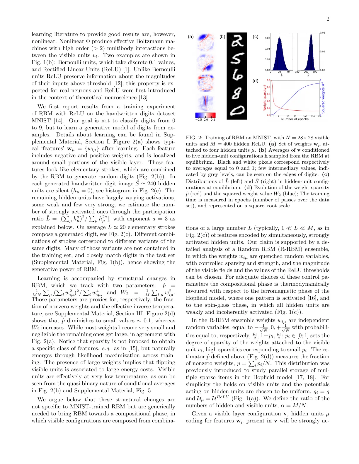
Emergence of Comp ositional Represen tations in Restricted Boltzmann Mac hines J. T ubiana, R. Monasson L ab or atoir e de Physique Th´ eorique, Ec ole Normale Sup ´ erieur e and CNRS, PSL R ese ar ch, Sorb onne Universit ´ es UPMC, 24 rue Lhomond,75005 Paris, F r anc e (Dated: March 6, 2017) Extracting automatically the complex set of features comp osing real high-dimensional data is crucial for ac hieving high p erformance in mac hine–learning tasks. Restricted Boltzmann Machines (RBM) are empirically known to b e efficient for this purp ose, and to b e able to generate distributed and graded represen tations of the data. W e characterize the structural conditions (sparsit y of the w eights, low effective temp erature, nonlinearities in the activ ation functions of hidden units, and adaptation of fields main taining the activity in the visible lay er) allowing RBM to op erate in such a comp ositional phase. Evidence is provided b y the replica analysis of an adequate statistical ensem ble of random RBMs and by RBM trained on the handwritten digits dataset MNIST. Recen t years hav e witnessed ma jor progresses in su- p ervised mac hine learning, e.g. in video, audio, im- age pro cessing,... [1]. Despite those impressive suc- cesses, unsup ervised learning, in which the structure of data is learned without a priori knowledge still presents formidable challenges. A fundamental question is how to learn probability distributions that fit well complex data manifolds in high-dimensional spaces [2]. Once learnt, suc h gener ative mo dels can be used for denoising, comple- tion, artificial data generation,... Hereafter w e focus on one imp ortant generativ e mo del, Restricted Boltzmann Mac hines (RBM) [3, 4]. In its simplest formulation a RBM is a Boltzmann mac hine on a bipartite graph, see Fig. 1(a), with a visible (v) la yer that represen ts the data, connected to a hidden (h) lay er meant to extract and ex- plain their statistical features. The marginal distribution o ver the visible la yer is fitted to the data through appro x- imate likelihoo d maximization [5–8]. Once the parame- ters are trained each hidden unit b ecomes selectiv ely ac- tiv ated by a sp ecific data feature; ow e to the bidirection- alit y of connections the probability to generate configu- rations of the visible la yer where this feature is present is, in turn, increased. Multiple combinations of num b ers of features, with v arying degrees of activ ation of the cor- resp onding hidden units allow for efficien t generation of a large v ariety of new data samples. How ev er, the exis- tence of suc h ‘comp ositional’ enco ding seems to depend on the v alues of the RBM parameters, suc h as the size of the hidden lay er [9]. Characterizing the conditions under whic h RBM can op erate in this compositional regime is the purp ose of the presen t work. In the RBM shown in Fig. 1(a) the visible la y er in- cludes N units v i , with i = 1 , . . . , N , c hosen here to b e binary (= 0 , 1). Visible units are connected to M hidden units h µ , through the w eigh ts { w iµ } . The energy of a configuration v = { v i } , h = { h µ } is defined through E [ v , h ] = − N X i =1 M X µ =1 w iµ v i h µ − N X i =1 g i v i + M X µ =1 U µ ( h µ ) , (1) where U µ is a p otential acting on hidden unit µ ; due FIG. 1: (a) Architecture of RBM. Visible ( v i , i = 1 , . . . , N ) and hidden ( h µ , µ = 1 , .., M ) units are connected through w eights ( w iµ ). (b) Activ ation functions Φ of Bernoulli, Lin- ear and Rectified Linear Units. The corresp onding p oten tials are U Lin ( h ) = h 2 2 ; U B er ( h ) = h θ B if h = 0 or 1, and + ∞ otherwise; U ReLU ( h ) = h 2 2 + h θ for h ≥ 0, + ∞ for h < 0. (c) The three regimes of op eration, see text. Blac k, grey and white hidden units symbolize, resp ectiv ely , strong, weak and n ull activ ations. to the binary nature of the visible units their p otential is fully characterized by a local field, g i in (1). Con- figurations are then sampled from the Gibbs equilibrium distribution associated to E , P [ v , h ] = exp( − E [ v , h ]) / Z , where Z is the partition function [3]. Giv en a visible configuration v the most likely v alue h µ of hidden unity µ is a function of its input I µ = P N i =1 w iµ v i : h µ = Φ µ ( I µ ), where the activ ation function Φ µ = ( U 0 µ ) − 1 as can b e seen from the minimization of E . Examples of Φ are shown in Fig. 1(b). When Φ is linear, i.e. for quadratic p oten tial U the probability P [ v , h ] is Gaussian in the hidden units, and the marginal distribu- tion P [ v ] of the visible configurations v can b e exactly computed [10]. It coincides with the equilibrium distribu- tion of a Boltzmann mac hine with a pairwise interaction matrix J ij = P µ w iµ w j µ , or, equiv alently , of a Hopfield mo del [11], whose M patterns w µ are the columns of the w eight matrix { w iµ } . Activ ation functions Φ empirically known in machine– 2 learning literature to p ro vide go o d results are, ho w ev er, nonlinear. Nonlinear Φ pro duce effectiv e Boltzmann ma- c hines with h igh order ( > 2) m ultib o dy in teractions b e- t w e en the visible units v i . Tw o examples are sho wn in Fig. 1(b): Bernoulli units, whic h tak e discrete 0,1 v alues , and Rectified Linear Units (ReLU) [1]. Unlik e B ern oulli units ReLU preserv e information ab out the magnitudes of their in puts ab o v e threshold [12]; t his prop ert y is ex- p ected for real neuron s and ReLU w ere first in tro duced in the con text of theoretic al neuroscience [13]. W e first rep ort results from a training exp erimen t of RBM with ReLU on the handwritten digits dataset MNIST [14]. Our goal is not to classify digits from 0 to 9, but to learn a generativ e mo del of digits from ex- amples. Details ab out learning can b e found in Sup- plemen tal Material, Section I. Figure 2(a) sho ws t yp i- cal ‘featur e s’ w µ = { w iµ } after l e arn ing. Eac h feature includes negativ e and p ositiv e w eigh ts, and is lo calized around small p ortions of the visible la y er. These fea- tures lo ok lik e elemen tary strok es, whic h are com bined b y the RBM to generate random digits (Fig. 2(b)). In eac h generated handwritten digit image ˆ S ' 240 hidden units are silen t ( h µ = 0), see histogram in Fig. 2(c). Th e remaining hidden units ha v e largely v arying activ ations, some w eak and fe w v ery stron g; w e estimate the n um- b er of strongly activ ated ones through the participation ratio ˆ L = [( P µ h a µ ) 2 / P µ h 2 a µ ], with exp onen t a = 3 as explained b elo w. On a v erage ˆ L ' 20 elemen tary strok e s comp ose a generated digit, see Fig. 2(c). Differen t com bi- nations of strok es corresp ond to differen t v arian ts of the same digits. Man y of those v arian ts are not con tained in the training se t , and closely matc h digits in the test set (Supplemen tal Mate r ial, Fig. 1(b)), hence s h o wing the generativ e p o w er of RBM. Learning is accompanied b y structural c hanges i n RBM, whic h w e trac k with t w o parameters: ˆ p = 1 M N P µ [( P i w 2 iµ ) 2 / P i w 4 iµ ] and W 2 = 1 M P i,µ w 2 iµ . Those parameters are pro xies for, resp ectiv ely , the frac- tion of nonzero w e igh ts and the effectiv e in v erse temp era- ture, see Suppl e men tal Material, Section I I I. Figure 2(d) sho ws that ˆ p diminishes to small v alues ∼ 0 . 1, whereas W 2 increases. While most w eigh ts b ecome v ery small and negligible the remaining ones get large, in agreemen t with Fig. 2(a). Notice that sparsit y is n ot imp osed to obtain a sp ecific class of features, e.g. as in [15], but naturally emerges through lik eliho o d maximization across train- ing. The pres ence of large w eigh ts implies that flippin g visible units is asso ciated to large energy costs. Visible units are effectiv ely at v ery lo w temp erature, as can b e seen f rom the quasi binary nature of conditional a v erages in Fig. 2(b) and Supplemen tal Materi al, Fig. 5. W e argue b elo w that these structural c hanges are not s p ecific to MNIST-trained RBM but are generically needed to bring RBM to w ards a comp ositional phase, in whic h visible configurations are comp osed fr om com bina- FIG. 2: T raining of RBM on MNIST, with N = 28 × 28 visible units and M = 400 hidden ReLU. (a) Set of w eigh ts w µ at- tac hed to four hidden units µ . (b) Av erages of v conditioned to fiv e hidden-unit configurations h sampled from the RBM at equilibrium. Blac k and white pixels corresp ond resp ectiv ely to a v erages equal to 0 and 1; few in termediary v alues, indi- cated b y grey lev els, can b e seen on the edges of digits. (c) Distributions of ˆ L (left) and ˆ S (righ t) in hidden-unit config- urations at equilibrium. (d) Ev olution of the w eigh t sparsit y ˆ p (red) and the sq u ared w eigh t v alue W 2 (blue); The training time is measured in ep o c hs (n um b er of passes o v er the data set), a nd represen ted on a square–ro ot scale. tions of a large n um b er L (t ypically , 1  L  M , as in Fig. 2(c)) of features enco ded b y sim ultaneously , strongly activ ated hidden units. Our claim is supp orted b y a de- tailed analysis of a Random RBM (R-RBM) ensem ble, in whic h the w eigh ts w iµ are quenc hed random v ariables, with con trolled sparsit y and strength , and the magnitude of the visible fields and the v alues of the ReLU thresholds can b e c hosen. F or adequate c hoices of thes e con trol pa- rameters th e comp ositional phase is thermo dynamically fa v oured with resp ect to the ferromagnetic phase of the Hopfield mo del, where one pattern is activ ated [16], and to the spin-glass phase, in whic h all hidden units are w eakly and incoheren tly activ ated (Fig. 1(c)). In the R-RBM ensem ble w e i gh ts w iµ are indep enden t random v ariables, equal to − 1 √ N , 0 , + 1 √ N with probabili- ties equal to, resp ectiv e ly , p i 2 , 1 − p i , p i 2 ; p i ∈ [0; 1] sets the degree of sparsit y of the w eigh ts attac hed to the visible unit v i , high sparsities corr e sp onding to small p i . The es- timator ˆ p defined ab o v e (Fig. 2(d)) meas u res the fraction of nonzero w eigh ts, p = P i p i / N . This distribution w as previously in tro duced to s tu dy parallel storage of m ul- tiple sparse items in the Hopfield mo del [17, 18]. F or simplicit y the fields on visib le units and the p oten tials acting on hidden u nits are c hosen t o b e uniform, g i = g and U µ = U R eLU (Fig. 1(a)). W e define the ratio of the n um b ers of hidden and visible un its , α = M / N . Giv en a visible la y er configuration v , hidden units µ co ding for features w µ presen t in v will b e strongly ac - 3 tiv ated: their inputs I µ = w µ · v will b e strong and p ositiv e, comparable to the pro duct of the norms of w µ ( ' √ p for l arge N ) and v (of the order of √ p N ), and, hence, will scale as m √ N , w h e r e m , called magnetiza- tion, is finite. Most hidden units µ 0 ha v e, ho w ev er, fea- tures w µ 0 essen tially orthogonal to v , and receiv e inpu ts I µ 0 fluctuating around 0, with finite v ariances. These scalings ensure that ˆ L defined ab o v e (Fig. 2(c)) will coin- cide with the n um b er L of strongly activ ated units when N → ∞ ; c ho osing exp onen t a = 2 in ˆ L rather than a = 3 w ould ha v e in tro duced biases coming from w eakly acti- v ated units (Supplemen tal Material, Section I I I.B). The t ypical ground state (GS) energy E (1) of R-RBM can b e computed with the re p lica metho d withi n the replica-symmetric Ansatz [16], as th e optim um of E GS = L 2 m 2 + α 2 ( q B + r C ) − 1 N X i √ α p i r (2) ×  H (1)  −  g + α 2 B p i + m W  / √ α p i r  W + α Z D z min h  U R eLU ( h ) − C 2 h 2 − z √ pq h  o v er the order parameters m, L, r , q , B , C (a v eraged o v er the quenc hed w eigh ts): m and L are, resp ectiv ely , the magnetization and the n um b er of feature-enco ding hid- den units, r is the mean squared activit y of the other hidden units, q = P i p i h v i i GS / ( N p ) is the w eigh ted ac- tivit y of the visible la y e r in the GS, and B , C are r e sp onse functions, i.e. deriv ativ es of the mean ac ti vit y of, resp ec- tiv ely , hidden and vi s ib le units with resp e ct to their in- puts [20]. In (2) D z = dz √ 2 π e − z 2 / 2 denotes the Ga u s sian measure, H ( k ) ( x ) = R x D z ( z − x ) k , and h·i W is the a v- erage o v er the sum W of L i.i.d. w eigh ts w iµ dra wn as ab o v e. W e first fix L , and optimize E GS o v er all the other or- der parameters. A t large α the only solution has m = 0, and corresp onds to t he Spin-Glass phase. F or in termedi- ate v alues of α , other s ol utions, with m > 0, exist. F or the sak e of simplicit y w e consider first the homoge n ous sparsit y case, with p i = p . W e sho w in Fig. 3(a), for fixed p = 0 . 1 and v arious v alues of L , the maximal v alue of α b elo w whic h a phase with L magnetized hidden u nits ex- ists. Imp ortan tly this critical v alue can b e made arbitrar- ily large b y increasing the R eLU threshold θ . This phe- nomenon is a consequence of the nonlinearit y of ReLU, and can b e understo o d as follo ws. The squared activit y r of non - magnetized hidden units ob eys the saddle-p oin t equation r = pq / (1 − C ) 2 × H (2) ( θ / √ pq ). The first factor is rem i nisc en t of th e expression r = 1 / (1 − C ) 2 arising for the Hopfield mo del (for whic h p = q = 1 at zero temp erature) [16], while the se cond factor comes from the n onlinearit y of ReLU. H (2) b eing a rapidly deca ying function of its argumen t large t hres h olds θ lead to small r v alues. As the lev el of crosstalk due to nonmagnetized hidden units diminishes larger ratios α can b e supp orted b y R-RBM without e n tering the glassy phase. Numerical sim ulations of R-RBMs at large α confirm the existence and (meta)stabilit y of phases with L nonzero magneti- zations (Fig. 3(b)). Moreo v er, the v alues of the a v erage normalized ma gn e ti z ation s ˜ m = m/ ( p/ 2) ∈ [0; 1] are in excellen t agreemen t with those found b y optimizing E GS . FIG. 3: Comp ositional regime in R-RBM. (a) Critical lines in the θ , α plane b elo w whic h L hidden units ma y b e strongly activ ated, calculated from the optimization of E GS (2). P a- rameters are p i = p = 0 . 1, g = − 0 . 02. (b) Comparison of theoretical (red crosses) and n umerical sim ulations ( N = 10 4 visible units, colored p oin ts) for the rescaled magnetizati ons ˜ m = m/ ( p/ 2)) as a function of the n um b er L of strongly activ ated hidden units in R-RBM. 7, 500 zero temp erature MCMC, eac h initialized with a visible configuration strongly o v erlapping with L = 1 , 2 , ... ‘features’, w ere launc hed; color co de indicates the probabilit y that the same L hidden units are magnetized after con v ergence (see b ottom scale), and the corresp onding a v erage magnetization ˜ m . The nature of the large– L phases and th e selection of the v alue of L are b est understo o d in the limit case of highly sparse connections, p  1. The R-RBM mo del ex- hibits an in teresting limit b eha viour, whic h w e call here- after c omp ositional phase. In this re gi m e the n um b er of strongly magnetized h idden units is un b ounded, and di- v erges as L = `/p , with ` > 0 and finite. The normalized GS energy e ` = E GS ( L = `/p ) /p is a nonmonotonous function of the in dex ` , see Fig. 4(a). Minimization of e ` leads to the selection of a w ell defined index ` ∗ . The mag - netizations of the ` ∗ /p strongly activ ated units, m = p 2 ˜ m , v anish linearly with p [26]. Nonmagnetized hidden units ha v e activities of the order of √ r ∼ √ p , and can b e sh ut- do wn b y c ho osing thresholds θ ∼ √ p ; hence crosstalk b e- t w ee n th os e units can b e s u ppress ed, allo wing for large relativ e size α of the hidden la y e r . The input receiv e d b y a visible uni t from the large n um b er of m agn e tized units is, after transmission through the dilute w eigh ts, of the order of L m p = 1 2 ` ∗ ˜ m p ; it can b e mo dulated b y a (p ositiv e or negativ e) field g ∼ p to pro duce an y finite activit y q in the visible la y er, as so on as the effectiv e temp erature gets b elo w ∼ p . The comp osition al phase comp etes with the ferromag- netic phase, in whic h ˜ m > 0 but e ` is a monotonously 4 gro wing function of ` (hence, ` ∗ = 0), and the spin glass phase, in whic h ˜ m = 0 and e ` do es not dep end on ` , see Fig. 4(a). The p hase diagram in the parameter space ( α , ˜ g = g p , ˜ θ = θ √ p ) will b e detailed in [20]. Briefly sp eak- ing, giv en α , ˜ θ should b e large enough (as in Fig. 3) and | ˜ g | should b e neither to o large to p enalize the ferromag- netic phase, nor to o small to a v oid the spin glass regime. FIG. 4: (a) . Beha viour of the GS energy e ` vs. ` = L × p in the p → 0 limit. P arameters: ˜ θ = 1 . 5, α = 0 . 5. (b) - (c) - (d) . Quan titativ e predictions in the comp ositional re gime of R-RBM compared to RBMs inferred on MNIST. Eac h p oin t represen t a ReLU RBM trained with v arious regularizations, yielding differen t w eigh t sparsities p . Solid lines depict pre- dictions found b y optimizing e ` (2), and dashed line exp ected fluctuations at finite siz e ( N ) and temp erature. (b) Av er- age n um b er L of activ e hidden units vs. p . (c) Av erage magnetization ˜ m vs. ` = L × p . (d) Distance (p er pixel) b e- t w een the pairs of visible configurations after con v ergence of zero-temp erature MCMC vs. relativ e distances in t he hidden- unit activ ation patterns. MCMC are initialized with all pairs of digits in MNIST; final visible configurations differ from MNIST digits b y ab out 7 pixels, b oth on the training and test sets, see Supplemen tal Material, Fig. 1. In all four panels pre- dictions for the homogeneous ( ˜ g = − 0 . 21) and heterogeneous ( ˜ g = − 0 . 1725, see Supplemen tal M aterial, Sectio n I I I.E) cases are sho wn in , resp ectiv ely , cy an and m agen ta. Characteristic prop erties of our comp ositional phase are confron ted to ReLU RBMs trained on MNIST in Fig. 4 (b,c). Compared to Fig. 2 w e add a regulariza- tion p enalt y ∝ P µ ( P i | w iµ | ) x to c on trol the final degree of sparsit y; the case x = 1 giv es standard L 1 regular- ization, while, for x > 1, the effectiv e p enalt y strength ∝ ( P i | w iµ | ) x − 1 increases with the w eigh ts, hence pro- moting homogeneit y among hidden u nits. After train- ing w e generate Mon te Carlo samples of eac h RBM at equilibrium, and monitor th e a v erage n um b er of activ e hidden units, ˆ L , and the normalize d magnetization, ˜ m . Figure 4(b) sho ws ˆ L vs. ˆ p , in go o d a gr e emen t with the R-RBM theoretical sc alin g L ∼ ` ? p . Figure 4(c) sho ws that ˜ m is a decreasing function of ` = ˆ L × ˆ p , as qualita- tiv ely predicted b y theory , but quan titativ ely differs from the prediction of R-RBM with homogeneous p . This dis- agreemen t c an b e partly explained b y the heteroge n e it ie s in the sparsities p i in RBMs trained on MNIST, e.g. units on the b or ders are connected to only few hidden units, whereas units at the cen ter of the grid are connected to man y . W e in tro duce a heterogeneous R-RBM mo del, where the distribution of the p i ’s is fitted from MNIST- trained RB M s (Supplemen tal Material, Section I I I.E). Its GS energy can b e calculated from (2), see Fig. 4(a) [20]. Results are sho wn in Fig. 4(b,c) to b e in go o d agreemen t with RBM trained on MNIST. RBMs, unlik e the Hopfield or mixture mo del, ma y pro- duce grad ually differen t visible configurations through progressiv e c hanges in the hidden-la y er activ ation pat- tern. R-RBMs enjo y the same prop ert y . W e compute, through a real-replica approac h [20], the a v erage Ham- ming distance d (p er pixel) b et w een the visible config- urations v (1) , v (2) minimizing the e n e r gy E (1) for t w o hidden configurations h (1) , h (2) sharing ( ` − δ ` ) /p hid- den u nits among the `/p strongly activ ated on e s. Fig- ure 4(d) sho ws that d monotonously increases fr om d = 0 for δ ` = 0 up to d = 2 q (1 − q ) (complete decorrelation of vis i ble units) f or δ ` = ` , in v ery go o d quan titati v e agreemen t with results for RBM trained on MNIST. The gradual c hange prop ert y has deep dynamical con- sequences. MCMC of MNIST-train e d RBM (vid e os a v ailable in Supplemen tal M ate r ial) sho w that gr adual c hanges ma y o ccasionally lead to another digit t yp e, b y passing thr ough w ell-dra wn, y et am biguous digits. The progressiv e replacemen t of feature-enco ding hidden units (small δ ` steps) along the transition path do es not in- crease m uc h t he energy , and the transition pro cess is fast compared to activ ate d hopping b et w een deep minima taking place in the Hopfield m o del. Our study is related to sev eral previous w orks. RB M s with linear activ ation function Φ coincide with the Hop- field mo del. In this framew ork m agn e ti z ed hi dden units iden tify retriev ed patterns, and α corresp onds to the capacit y of th e autoasso ciativ e memory . Tso d yks and F eigel’man sho w ed ho w the critical capacit y (for single pattern retriev al) could b e dramatically increased with sparse w eigh ts ( p  1) and appropriate tun ing of the fields g i [21]; ho w ev er this effec t could b e ac hiev ed only with v anishingly lo w activities q . Agliari and collab ora- tors sho w ed in a series of pap ers [17, 18] that m ultiple sparse patterns could b e sim ultaneously retriev ed in the case of linear Φ and v anishin g capacit y α = 0 (finite M ). Finite capacit y α ∼ c − 2 could b e ac hiev ed at zero 5 temp erature in the limit of extreme sparsit y , p = c/ N , only [19]; for MNIST p ' 0 . 1 and N = 784 would give α ∼ 2 . 10 − 4 . Our w ork shows that large v alues of α can b e reached even with mo derate sparsity p (as in realistic situations, see Fig. 2) provided that nonlinear Φ (ReLU) and appropriate threshold v alues θ are considered. The presence of the fields g i acting on the visible units (absen t in the v i = ± 1 mo del of [17–19]), is also crucial for the existence of our comp ositional phase as explained ab ov e. It would b e interesting to extend our work to more than one la y ers of hidden units, or to other t ypes of nonlinear Φ. While n umerical studies of RBMs with Bernoulli hidden units show no qualitative c hange com- pared to ReLU, choosing Φ( h ) gro wing asymptotically faster than h could affect the nature of the extracted features [23]. An important challenge w ould be to un- derstand the training dynamics, i.e. how hidden units gradually extract features from data prototypes. Ac kno wledgements. W e are grateful to C. Fisher and G. Semerjian for useful discussions. This w ork w as partly funded b y the CNRS-Inph yniti Inferneuro and the HFSP R GP0057/2016 pro jects, and b enefited from the supp ort of NVIDIA Corporation with the donation of a T esla K40 GPU card. [1] Y. LeCun, Y. Bengio, J. Hin ton, Natur e 521 , 436-444 (2015). [2] Y. Bengio, A. Courville, P . Vincen t, IEEE tr ansactions on p attern analysis and machine intel ligenc e 35 , 1798- 1828 (2013). [3] P . Smolensky , Chapter 6: Information Processing in Dy- namical Systems: F oundations of Harmony Theory , in Par al lel Distribute d Pr o c essing: Explor ations in the Mi- cr ostructur e of Co gnition, V olume 1: F oundations , MIT Press, 194-281 (1986). [4] R. Salakhutdino v, A. Mnih, G. Hinton, Pr o c e e dings of the 24th international confer enc e on Machine le arning , p. 791-798 (2007). [5] G. Hinton, Momentum 9 , 926 (2010). [6] T. Tieleman, Pr o c e e dings of the 25th international c on- fer enc e on Machine le arning , pp. 1064-1071 (2008). [7] G. Desjardins, A. Courville, Y. Bengio, P . Vincent, O. Delalleau, Pr o c e edings of the 13th International Confer- enc e on Artificial Intel ligenc e and Statistics , pp. 145-152 (2010). [8] M. Gabrie, E.W. T ramel, F. Krzak ala, A dvanc es in Neu- r al Information Pr o c essing Systems , pp. 640-648 (2015). [9] A. Fischer, C. Igel, Iber o americ an Congress on Pattern R e c o gnition , pp. 14-36 (2012). [10] A. Barra, A. Bernacc hia, E. San tucci, P . Con tucci, Neur al Networks 34 , 1-9 (2012). [11] J.J. Hopfield, Pr oc. Nat. A c ad. Sci. USA 79 , 2554 (1982). [12] V. Nair, G.E. Hin ton, Pr o c e e dings of the 27th Inter- national Confer enc e on Machine L e arning , p. 807-814 (2010). [13] A. T reves, J. Comp. Neur osci. 2 , 259-272 (1995). [14] Y. LeCun, C. Cortes, C.J. Burges, The MNIST database of handwritten digits (1998). [15] B.A. Olshausen, D.J. Field, Natur e 381 , 607-609 (1996). [16] D.J. Amit, H. Gutfreund, H. Sompolinsky , Phys. R ev. L ett. 55 , 1530 (1985). [17] E. Agliari, A. Barra, A. Galluzzi, F. Guerra, F. Moauro, Phys. R ev. L ett. 109 , 268101 (2012). [18] E. Agliari, A. Annibale, A. Barra, A.C.C. Co olen, D. T antari, J. Phys. A 46 , 415003 (2013). [19] P . Sollich, D. T antari, A. Annibale, A. Barra, Phys. R ev. L ett. 113 , 238106 (2014). [20] J. T ubiana, R. Monasson, in pr ep ar ation (2017). [21] M. Tso dyks, M.V. F eigel’man, Eur ophys. L ett. 6 , 101-105 (1989). [22] R. Salakhutdino v, I. Murray , Pr o ce e dings of the 25th in- ternational c onfer enc e on Machine le arning , pp. 872-879 (2008). [23] D. Krotov, J.J. Hopfield, arXiv:1606.01164 (2016). [24] See Supplemental Material [url], which includes Ref [25]. [25] Theano Developmen t team Theano Developmen t T eam. arXiv:1605.02688. (2016). [26] Solutions with nonhomogeneous magnetizations m µ , v arying from one strongly activ ated hidden unit to an- other, give additional contributions to E GS of the order of p 2 with resp ect to the homogeneous solution m µ = m , and do not affect the v alue of e ` [20]. Supplemen tal Material Emergence of Comp ositional Represen tations in Restricted Boltzmann Mac hines J. T ubiana, R. Monasson I. TRAINING RBMS ON MNIST A. Dataset preparation and initial conditions • In MNIST, eac h pixel has a v alue b et w een 0 and 255. W e binarize it b y thresholding ≥ 128. The 28 × 28 binary images are flattened to a N = 784 vector with binary v alues. • The dataset is split in a training (60,000 instances) and a test (10,000 instances) sets • The weigh ts w iµ are randomly initialized at ± W , where W = q 0 . 1 N ; this c hoice corresp onds to initial temp erature and weigh t sparsity : T (0) = 10 and p (0) = 1 (see section I II). • The initial field v alues are g 0 i = log h h v i i M N I S T 1 −h v i i M N I S T i , where h v i i M N I S T denotes the a v erage of pixel i o ver the training data • F or ReLU, the thresholds θ µ are all initially set to 0 B. Learning algorithms A RBM is associated to a probability distribution P [ v , h ) = e − E [ v , h ] Z , where the energy E is defined in the main text. The marginal distribution, P [ v ] = R Q dh µ P [ v , h ) is fitted to the data b y likelihoo d maximization. Giv en data instances x r , r ∈ { 1 , D } , the log-likelihoo d is : log L W , g , θ = 1 D D X r =1 log [ P [ x r | W , g , θ | ] (1) Where W is the matrix of weigh ts, g is the vector of visible la yer fields and θ is the v ector of hidden units thresholds. Lik eliho o d maximization is implemented by stochastic gradien t descen t, with the difficult y that extensiv e Mon te Carlo sim ulations are required to compute the gradient [1, 2]. F or the RBM of Fig. 2 in the main text, w e used P ersistent Con trastive Divergence [3] with • 20 mini-batch size • 100 p ersisten t chains • 1 Gibbs step betw een each update • 200 ep o c hs (600 000 updates in total) • Initial learning rate of λ i = 5 10 − 3 , decaying geometrically (decay starts after 60 ep o c hs) to λ f = 5 10 − 4 PCD is known to be inaccurate tow ard the end of learning, b ecause the parameters evolv e to o fast with resp ect to the the mixing rate of the Marko v chains. The regularized RBM of main text, Fig. 4 (b,c), were trained with a more efficien t algorithm, v ariant of Adaptive P arallel T emp ering [4, 5] with • 100 mini-batch size • 100 p ersisten t chains • 10 replicas 2 FIG. 1: (a) Ev olution throughout training of the d ata loglik eliho o d (left scale) and pseudo-loglik eliho o d (righ t scale) computed o v er the training and test sets. (b) Ev olution of the n u m b e r of distinct lo cal maxima of P W ( v ) (left scale) and the distance to the original sample (righ t scale, for train and test set) are displa y ed. • 1 Gibbs step b et w een eac h up date • 150 ep o c hs (90 000 up dates in total) • Initial learning rate of λ i = 10 − 2 , deca ying geometrically (deca y starts after 90 ep o c hs) to λ f = 10 − 4 C. Monitoring the learning W e monitor the ev olution of the lik eliho o d and of the pseudo-lik eliho o d of the train and test d ata sets throughout learning, see Fig. 1(a). The c hoice of parameters made learning slo w, but ensured that the lik elih o o d increased steadily throughout training. The lik eliho o d requires appro ximate computation of the mo del part ition fu nction; Annealed Imp ortan c e Sampling [6] w as used. P arameters : n β = 10000 in v erse temp eratures with an adaptiv e spacing [5], n r uns = 1. Additionnaly , w e can lo ok at the probab ilit y landscap e P W ( v ) throughout l e arn ing. F or eac h of the 70k MNIST sam p le s, a gradien t asce n t on P W ( v ) is p erformed un til c on v ergence to a lo cal maxim um; the n um b er of distinct lo cal m axi m a of P W ( v ) and the distance to the original sample are measured. As training go es, more lo cal maxima app ear, and they get closer to the training samples; lo cal maxima also app ear close to the te st set, whic h sho ws that RBM generalize w ell. D. Con troling w eigh t sparsit y with regularization T o con trol t he w eigh t sparsit y p , a regularization p enalt y is add e d to the log lik eliho o d log L W , g , θ : Cost = − log L W , g , θ + L ( x ) L ( x ) = λ x x X µ " X i | w iµ | # x − ∂ Cost ∂ w iµ = ∂ ∂ w iµ log L W , g , θ − λ x   X j | w j µ |   x − 1 sign( w iµ ) (2) The case x = 1 is the usual L 1 p enalt y and p erforming gradien t descen t with λ 1 > 0 is kn o wn to reduce the n um b er of non-zero w eigh ts w iµ . Ho w ev er, exp erimen ts sho w that the outcome is in homoge n e ou s with resp ect to the hidden units: some hidden units are w eakly affected b y the p e n alt y , whereas som e end up completely disconnected from the visible la y er, making them useless, see Fig. 2. T o main tain homogeneit y among the hidden units, w e pic k x = 2 or x = 3. As can b e seen from the expression of the gradien t, it is equiv alen t to a usual L 1 p enalt y , but with a deca y rate adaptiv e to eac h hidden unit: hidden units strongly (resp. w eakly) coupled to the visible la y er (large P i | w iµ | ) are strongly (resp. w eakly) regularized, th us increasing the homogeneit y among hidden units. 3 FIG. 2: Subset of 12 w eigh t features pro du c ed b y training on MNIST, regularized with L 1 , λ 1 = 10 − 3 (top panel), and L 2 , λ 2 = 3 . 10 − 5 (b ottom panel). Both ha v e o v erall sparsit y p ∼ 0 . 036, but th e latter is more homogeneously distributed across hidden units. FIG. 3: Six indep enden t Mon te Carlo Mark o v Chains realization for a RBM trained on MNIST, extracted f rom the attac hed vid e os, see text. I I. SAMPLING FR OM RBMS RBM c an b e s ampled b y Mark o v Chains Mon te Carlo. Du e to the conditional indep endence prop ert y , Gibbs sampling can b e p e rf orme d b y alternativ e sampling of h from P [ h | v ], then v from P [ v | h ] [1, 2]. A. MCMC Videos The t w o videos in Supplemen tary Material presen t visualize MCMC runs from RBM trained on MNIST with Bernoulli, Gaussian, ReLU hidden units. Eac h square depicts a Mark o v c hain s tar te d from a random initial condition. 20 Gibbs steps are p erformed b et w een eac h image, and eac h c hain is 500 images long. See Fig. 3 for a snapshot. 4 FIG. 4: T en Monte Carlo Marko v Chains realizations at differen t inv erse tempe ratures, coupled b y replica exchange. The plots shows the conditional expectations of visibile units, E [ v | h ], for thermalized hidden-unit activities, h . B. Estimating thermal a v erages with MCMC Sampling at thermal equilibrium is required to estimate the v alues of order parameters ( L , S , q , ˜ m ,...). Since RBM trained on MNIST effectively op erate at lo w temperature (en trop y of 0.1 bits/pixel) the MCMC mixing rate is p o or, and long sim ulations would b e required for eac h of the ∼ 100 RBMs trained. T o ov ercome this issue we use an Adaptive Parallel T emp ering (also kno wn as Replica Exc hange) sampling algorithm, with 10 replicas [4, 5]. Observ ables are av eraged ov er 100 independent Mark o v Chains, each b eing first thermalized for 500 Gibbs up dates, then run for another 100 Gibbs updates (10K samples in total). C. Estimating order parameters of R-RBM with zero temp erature MCMC R-RBM are studied analytically in the zero-temperature limit; this limit can b e sim ulated as w ell. The energy E [ v , h ] of a configuration v , h is giv en b y Eqn. (1) in main text, and defines the Gibbs distribution P β [ v , h ] = exp( − β E [ v , h ] / Z ( β ), where β = 1 T is the inv erse temperature. As β increases, P β [ v , h ] is more and more peaked around the minimum of E . In the limit β → ∞ , a dynamical Gibbs step b ecomes deterministic : h µ ← arg min h " U µ ( h ) − h X i w µi v i # ≡ Φ µ " X i w iµ v i # v i ← arg min v " − g i v − v X µ w µi h µ # ≡ Θ " g i + X µ w iµ h µ # , (3) where Θ is the Heaviside function, and Φ µ is the resp onse function (Fig. 1(b) in main text).Starting from a configu- ration, such zero-temperature Mark ov Chain runs until conv ergence to a lo cal minim um of E . In practice, to make finite-size corrections to our mean-field theory small, we considered RBMs with up to N ∼ 10 4 visible units. Such large R-RBM were simulated using a nVidia T esla K40 GPU, programmed with Theano [7]. 5 D. Finding lo cal maxima of P [ v ] Giv en an RBM with energy defined as ab ov e, the marginal P [ v ] is characterized by a Gibbs distribution and a free energy : P [ v ] = Z Y µ dh µ 1 Z e − E [ v , h ] = 1 Z e − F [ v ] F [ v ] = − X i g i v i + X µ U ef f µ X i w iµ v i ! U ef f µ ( x ) = − log  Z dh e − U µ ( h )+ xh  (4) In order to find the lo cal maxima of P [ v ] ( i.e. the lo cal minima of F [ v ] ) , we mo dify it b y introducing an in verse temp erature β : P β [ v ] = 1 Z ( β ) e − β F [ v ] Z ( β ) = X v e − β F [ v ] (5) Sampling from this distribution at β 6 = 1 is not trivial, as P β [ v ] is not the marginal distribution of P β [ v , h ] when β 6 = 1. While sampling from P 1 [ v ] is easy , as one can simply sample from the joint distribution P 1 [ v , h ] using Gibbs steps, this is not true for β 6 = 1; in particular the local maxima of P β [ v , h ] are not equiv alen t to those of P β [ v ]. W e notice how ever that when β ≥ 1 is an integer, P β [ v ] can b e in terpretated as the β = 1 distribution of another RBM P 0 1 [ v ] with β M hidden units (eac h hidden unit is replicated β times) and visible fields g 0 = β g . Sampling from such RBM can be done as following : • Compute the hidden la y er inputs P i w iµ v i • Sample indep enden tly β replicas h r µ of h µ from P 1 [ h µ | v ] • Compute the visible la y er inputs I i = P β r =1 P µ w iµ h r µ • Sample v i from the Bernoulli distribution B er n h β ( g i + 1 β I i ) i When β → ∞ , 1 β P β r =1 h r coincides with the conditional av erage of h given v , E [ h | v ]. Therefore, the zero temp er- ature sampling Gibbs step for the free energy is equiv alent to : h µ ← E [ h µ | v ] v i ← Θ " g i + X µ w iµ h µ # (6) I II. NUMERICAL PRO XIES F OR CONTR OL AND ORDER P ARAMETERS Sev eral control and order parameters are w ell defined for R-RBM in the thermo dynamical limit, but not for typical RBM trained on data. F or R-RBM instances, the av erage weigh t sparsit y p is well defined b ecause the weigh ts take only three distinct v alues {− 1 √ N , 0 , 1 √ N } , but for RBM trained on data, the weigh ts w iµ are never exactly equal to zero. Similarly , the num ber of strongly activ ated hidden units L is well-defined for R-RBM in the thermo dynamic limit N → ∞ b ecause their activity scales as √ N ; but in general, all hidden units hav e finite activ ation. Proxies are therefore required to compare theoretical and numerical results. W e consider ’consistent’ proxies, giving bac k (in the large size limit), the original parameters for RBMs drawn from the R-RBM ensem ble. 6 A. P articipation Ratios P R P articipation ratios are used to estimate num bers of nonzero comp onen ts in a vector, while a v oiding the use of arbitrary thresholds. The Participation Ratio ( P R a ) of a v ector x = { x i } is P R a ( x ) = ( P i | x i | a ) 2 P i | x i | 2a If x has K nonzero and equal (in modulus) components PR is equal to K for any a . In practice w e use the v alues a = 2 and 3: the higher a is, the more small comp onen ts are discoun ted against strong comp onen ts in x . B. Num b er L of active hidden units In b oth numerical simulations of R-RBM and on RBM trained on MNIST, w e estimate L , for a giv en hidden-unit configuration h , through ˆ L = P R 3 ( h ) T o understand the c hoice a = 3, consider a t ypical activ ation configuration h for a R-RBM : h µ =  m √ N if 1 ≤ µ ≤ L , √ r x µ if L + 1 ≤ µ ≤ M , (7) where the magnetization m and mean square activit y r are O (1), and x µ are random v ariables with zero mean, and ev en moments of the order of unity . The first L hidden units are strongly activ ated ( O ( √ N ) activity), whereas the remaining N − L others are not (activ ations of the order of 1). Here, w e assume L to b e finite as N → ∞ . One computes : P R 2 ( h ) ∼ ( Lm 2 N + ( N − L ) r ) 2 Lm 4 N 2 + ( N − L ) r 2 = L × (1 + N − L N r Lm 2 ) 2 1 + N − L N 2 r 2 Lm 4 − → N →∞ L (1 + r Lm 2 ) 2 , P R 3 ( h ) ∼ ( Lm 3 N 3 / 2 + ( N − L ) r 3 / 2 ) 2 Lm 6 N 3 + ( N − L ) r 3 = L × (1 + N − L N 3 / 2 r 3 / 2 Lm 3 ) 2 1 + N − L N 3 r 3 Lm 6 − → N →∞ L . (8) Hence choosing coefficient a = 3 ensures that the participation ratio (a) do es not take into account the weak activ ations in the thermo dynamical limit, and (b) conv erges to the true v alue L if all magnetizations are equal. C. Normalized Magnetizations ˜ m Giv en a RBM and a visible lay er configuration, we define the normalized magnetization of hidden unit µ as the normalized ov erlap b et ween the configuration and the w eigh ts attached to the unit: ˜ m µ = P i (2 v i − 1) w iµ P i | w iµ | ∈ [ − 1 , 1] This definition is consistent with the Hopfield mo del. F or R-RBM, we also ha ve, in the thermodynamical limit, ˆ m µ = 2 I µ p √ N , where I µ is the input receiv ed by the hidden unit from the visible lay er; m µ is O (1) for strongly activ ated hidden units, and O ( 1 √ N ) for the others. F or a giv en configuration v , with ˆ L activ ated hidden units, the normalized magnetization of the activ ated hidden units ˜ m = m p/ 2 can b e estimated as the av erage of the ˆ L highest magnetizations ˆ m µ . D. W eigh t sparsit y p A natural wa y to estimate the fraction of non-zero w eights w iµ w ould be to coun t the n umber of weigh ts with absolute v alue ab ov e some threshold t . How ev er, there is no simple satisfactory choice for t . Indeed, the fraction of 7 FIG. 5: (a) Histogram of ˜ p i = p i p v alues , across all visibl e units and RBMs inferred on MNIST. (b) Av erage ac r o ss all RBM of ˜ p i = p i p , for eac h visible u nit non-zero w eigh ts should not dep end on the scale of the w eigh ts, i.e. it should b e in v arian t und e r the global rescaling transformation { w iµ } → { λ w iµ } . As the scale of w eigh ts v ary from RBMs to RBMs and, for eac h RBM, across training it app ears difficult to select an appropriate v alue for t . A p ossibilit y w ould b e to use a threshold adapted to eac h RBM, e.g. t ∝ κ q W 2 M , where κ w ould b e some small n um b er. Our exp erimen ts sho w that it is not accurate enough, due to the scale disparities across the hidden–unit w eigh t v ectors w µ . Rather than adapting thresholds to eac h hidden unit of eac h RBM, w e use P articipation Ratios, whic h naturally enjo y the scale in v ar iance p rop ert y . W e estimate the fraction of nonzero w eigh ts through ˆ p = 1 M N X µ P R 2 ( w µ ) F or R-RBM with w iµ ∈ [ − W 0 , 0 , W 0 ] with corresp onding probabilities [ p 2 , 1 − p, p 2 ], the estimator is c on s isten t: ˆ p = p . E. W eigh ts heterogeneities As seen from the features of Fig. 2 in the main text, not all visible units are equally c on nec ted to the hidden la y er. T o b etter capture this effect, one can study R-RBM with an y arbitrary distribution of p i . Analogously to the homogeneous case a high sparsit y limit is obtained when the a v erage sparsit y , p = 1 N P i p i , v anishes. W e define the distribution of the ratios ˜ p i = p i p in the p → 0 limit. In practice the ratios are estim at e d through ˜ p i = P i w 2 iµ 1 M P i,µ w 2 iµ . (9) F or a heterogeneous R-RBM, w e ha v e consisten tly ˜ p i = ˆ p i p = p i p . Lo ok ing at the histogram of v alues of ˜ p i across all RBM inferred on MNIST, w e fi nd a non-negligible spread around one, see Fig. 5. W e also displa y f or eac h visible unit i the a v erage of ˜ p i accross all RBM inferred; w e can see that the visible units at the b order are indeed the least connected (smaller ˜ p i ), whereas the ones at the cen ter are strongly connected (larger ˜ p i ). F. Effectiv e T emp erature T Although RBM distributions are alw a ys defined at temp erature T = 1, the effectiv e temp eratur e is not 1. This is v ery m uc h lik e in the Ising mo del : the b eha vior of the system dep ends on an effectiv e temp erature ˆ T = T J where 8 FIG. 6: Conditional means E [ v | h ] for t w o hidden un its configurations sampled at equilibrium. Most pixels v i are frozen, with E [ v i | h ] ∈ { 0 , 1 } J is the coupli ng strength; a lo w effectiv e temp erature phase correp ond to high v alues of J . F or ReLU RBM, th e probabilit y distribution of configurations at temp erature T is defined as : P w [ v , h ] = e − E [ v , h ] T with E [ v , h ] T = − X i g i T v i + X µ h 2 µ 2 T + h µ θ µ T ! − X i,µ w iµ T v i h µ . (10) Let ¯ h = h √ T . The probabilit y can b e rewritten as P [ v , ¯ h ] = e − ¯ E [ v , ¯ h ] with ¯ E ( v , ¯ h ) = − X i g i T v i + X µ ¯ h 2 µ 2 + ¯ h µ θ µ √ T ! − X i,µ w iµ √ T v i ¯ h µ . (11) Since th e marginal P [ v ] is not affected b y the c hange of v ariable, a ReLU RBM at temp erature T is th e r e f ore equiv alen t to another ReLU RBM at temp erature T = 1, with new fields, thresholds and w eigh ts : ¯ g = g T , ¯ θ = θ √ T , ¯ w = w √ T . Therefore, c hanging the temp erature is equiv alen t to rescaling the par am eters, and in turn , the effectiv e temp erature of a giv en RBM can b e deduced from the amplitude of its w eigh ts. F or a R-RBM at temp erature T : W 2 = 1 M X µ,i ¯ w 2 iµ ∼ N →∞ p T . W e therefore estimate the temp erature of a giv en RBM through ˆ T = ˆ p 1 M P µ,i w 2 iµ . F rom this definition, it can b e seen that the lo w temp erature r e gime of the comp ositional regime, T  p , is equiv alen t to W 2  1. In RBM trained on MNIST, w e t ypically find W 2 ∼ 7 G. Fields g Similarly to t he w eigh ts, the fields g i and normalized field s could b e estimated resp e ctiv ely as: ˆ g i = ˆ T ¯ g i ˆ ˜ g i = ˆ T ˆ p ¯ g i = ¯ g i 1 M P µ,i w 2 iµ (12) A naiv e estimate for the n ormalize d field ˜ g w ould b e to a v erage the fields: ˆ ˜ g = 1 N P i ˆ ˜ g i . It is ho w ev e r not really meaningful, as th e ˆ ˜ g i are extremely h e terogeneous: for instance, the mean v alue o v er the sites i of a single RBM is 9 equal to − 0 . 48, and is comparable to the standard deviation, 0 . 40. This range of v ariation spans all the phases of R-RBM. T o achiev e quantitativ e predictions, we instead adjust the R-RBM parameter g so that q , the mean v alue of v i in the visible lay er, av eraged ov er thermal fluctuations and quenched disorder, matc hes the v alue 0 . 132 obtained from MNIST data. F or the plots of Figure 4 in the main text, this giv es ˆ g ˆ p = − 0 . 1725 for homogeneous R-RBM, and ˆ g ˆ p = − 0 . 21 for heterogeneous R-RBM. H. Thresholds θ The thresholds and normalized thresholds can be estimated as ˆ θ µ = p ˆ T ¯ θ µ ˆ ˜ θ µ = s ˆ T ˆ p ¯ θ µ = ¯ θ µ q 1 M P µ,i w 2 iµ (13) Again, a naiv e estimate for the normalized threshold ˜ θ w ould b e the av erage ˆ ˜ θ = 1 M P µ ˆ ˜ θ µ but this estimate is not meaningful. Indeed, contrary to the R-RBM case, the inputs I µ of the hidden units µ are not ev enly distributed around zero: E [ I µ ] 6 = 0. Hence, even if the threshold is equal to zero, the activ ation probability can b e differen t from 0.5. W e take this effect into account by substracting the av erage v alue of the inputs from the av erage of θ , and find that the difference is equal to 0 . 33, with standard deviation 1 . 11. This range of v alue for θ again spans all phases. In order to use a well-defined v alue, w e c ho ose θ such that the critical capacit y α R − RB M c ( ` max ) = 0 . 5, where ` max ∼ 1 . 5 is the maximum av erage index n umber observed across all RBMs trained for Fig. 4 in the main text. This estimation giv es ˆ ˜ θ ∼ 1 . 5. [1] A. Fischer, C. Igel. Ib er o americ an Congr ess on Pattern R e c o gnition , pp. 14-36 (2012). [2] G. Hinton. Momentum 9 , 926 (2010). [3] Tieleman, T. Pr o c e e dings of the 25th international c onfer enc e on Machine le arning , pp. 1064-1071 (2008, July). [4] Desjardins, G., Courville, A., Bengio, Y., Vincen t, P ., Delalleau, O. Pr o c e e dings of the 13th International Confer enc e on Artificial Intel ligenc e and Statistics , pp. 145-152 (2010). [5] J. T ubiana, R. Monasson, in pr ep ar ation (2017). [6] Salakh utdinov, R., & Murray , I. In Pr o c e e dings of the 25th international c onfer enc e on Machine le arning (pp. 872-879). (2008, July) [7] Theano Developmen t T eam. Theano: A Python framework for fast computation of mathematical expressions, arXiv pr eprint arXiv:1605.02688 . (2016).