Spectral model selection in the electronic measurement of the Boltzmann constant by Johnson noise thermometry

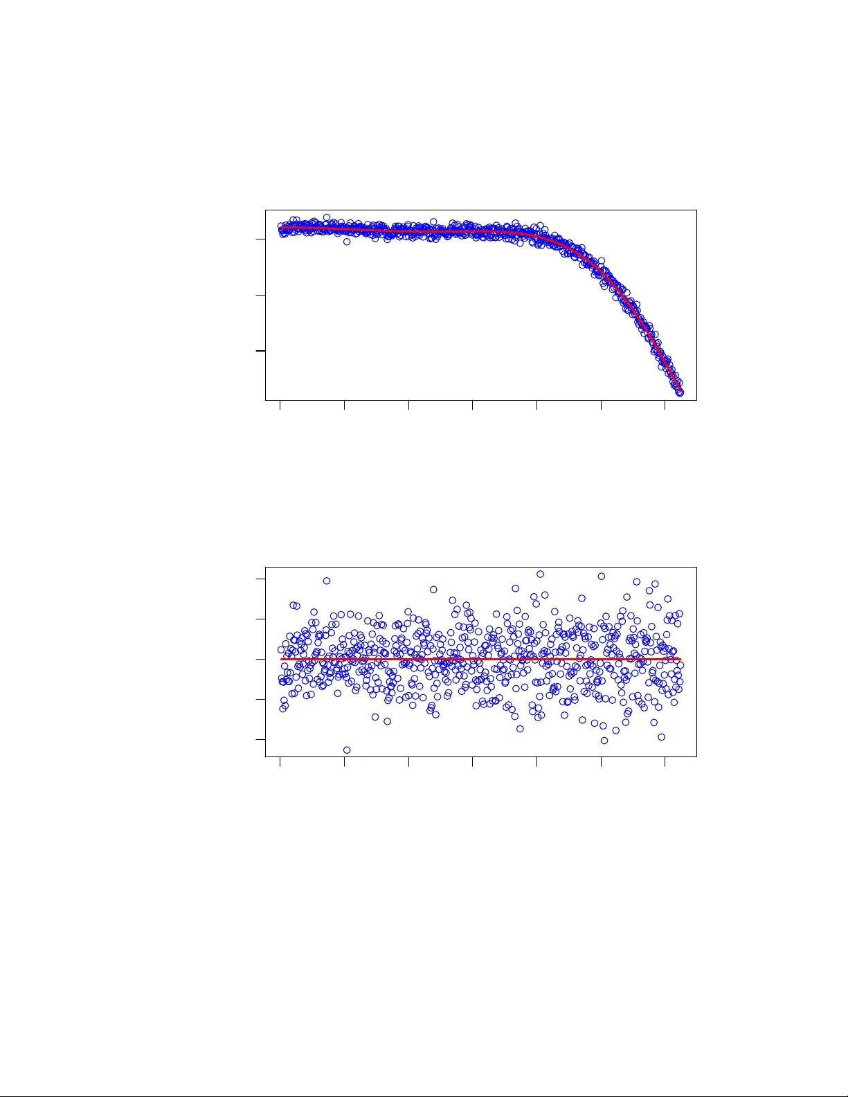
Spectral model selection in the electr onic measur ement of the Boltzmann constant by J ohnson noise thermometry K evin J Coakley 1 , Jifeng Qu 2 1 National Institute of Standards and T echnology (NIST), Boulder , CO 80302 USA 2 National Institute of Metrology (NIM), Beijing 100029, Peoples Republic of China E-mail: kevin.coakley@nist.gov 1. Abstract In the electronic measurement of the Boltzmann constant based on Johnson noise thermometry , the ratio of the power spectral densities of thermal noise across a resistor at the triple point of water , and pseudo-random noise synthetically generated by a quantum-accurate v oltage-noise source is constant to within 1 part in a billion for frequencies up to 1 GHz. Gi ven kno wledge of this ratio, and the values of other parameters that are kno wn or measured, one can determine the Boltzmann constant. Due, in part, to mismatch between transmission lines, the experimental ratio spectrum v aries with frequenc y . W e model this spectrum as an e ven polynomial function of frequency where the constant term in the polynomial determines the Boltzmann constant. When determining this constant (of fset) from experimental data, the assumed complexity of the ratio spectrum model and the maximum frequency analyzed (fitting bandwidth) dramatically affects results. Here, we select the complexity of the model by cross-v alidation – a data-dri ven statistical learning method. For each of many fitting bandwidths, we determine the component of uncertainty of the of fset term that accounts for random and systematic effects associated with imperfect knowledge of model complexity . W e select the fitting bandwidth that minimizes this uncertainty . In the most recent measurement of the Boltzmann constant, results were determined, in part, by application of an earlier version of the method described here. Here, we extend the earlier analysis by considering a broader range of fitting bandwidths and quantify an additional component of uncertainty that accounts for imperfect performance of our fitting bandwidth selection method. For idealized simulated data with additi ve noise similar to experimental data, our method correctly selects the true complexity of the ratio spectrum model for all cases considered. A new analysis of data from the recent experiment yields e vidence for a temporal trend in the offset parameters. K eyw ords: Boltzmann constant, cross-v alidation, Johnson noise thermometry , model selection, resampling methods, impedance mismatch 2. Introduction There are v arious experimental methods to determine the Boltzmann constant including acoustic gas thermometry [1],[2],[3]; dielectric constant gas thermometry [4],[5], [6], [7], Johnson noise thermometry Spectral model selection in the electr onic measur ement of the Boltzmann constant by Johnson noise thermometry 2 (JNT) [8], [9], [10], and Doppler broadening [11], [12]. COD A T A (Committee on Data for Science and T echnology) will determine the Boltzmann constant as a weighted a v erage of estimates determined with these methods. Here, we focus on JNT experiments which utilize a quantum-accurate voltage-noise source (QVNS). In JNT , one infers true thermodynamic temperature based on measurements of the fluctuating voltage and current noise caused by the random thermal motion of electrons in all conductors. According to the Nyquist law , the mean square of the fluctuating v oltage noise for frequencies belo w 1 GHz and temperature near 300 K can be approximated to better than 1 part in billion as < V 2 > = 4 k T R ∆ f , where k is the Boltzmann constant, T is the thermodynamic temperature, R is the resistance of the sensor , and ∆ f is the bandwidth o ver which the noise is measured. Since JNT is a pure electronic measurement that is immune from chemical and mechanical changes in the material properties of the sensor , it is an appealing alternati ve to other forms of primary gas thermometry that are limited by the non-ideal properties of real gases. Recently , interest in JNT has dramatically increased because of its potential contribution to the “Ne w SI” (Ne w International System), in which the unit of thermodynamic temperature, the kelvin, will be redefined in 2018 by fixing the numerical v alue of k . Although almost certainly the value of k will be primarily determined by the values obtained by acoustic gas thermometry , there remains the possibility of unkno wn systematic ef fects that might bias the results, and therefore an alternativ e determination using a different physical technique and different principles is necessary to ensure that any systematic effects must be small. T o redefine the kelvin, the Consultati ve Committee on Thermometry (CCT) of the International Committee for W eights and Measures (CIPM) has required that besides the acoustic gas thermometry method, there must be another method that can determine k with a relati ve uncertainty below 3 × 10 − 6 . As of now , JNT is the most likely method to meet this requirement. In JNT with a QVNS, [10], according to ph ysical theory , the Boltzmann constant is related to the ratio of the power spectral density (PSD) of noise produced by a resistor at the triple point of water temperature and the PSD of noise produced by a QVNS. For , frequencies belo w 1 GHz, this ratio is constant to within 1 part in 10 9 . The physical model for the PSD for the noise across the resistor is S R where S R = 4 k T W X R R, (1) T W is the temperature of the triple point of water , X R is the resistance in units of the v on Klitzing resistance R K = h e 2 where e is the charge of the electron and h is Planck’ s constant. The model for the PSD of the noise produced by the QVNS, S Q , is S Q = D 2 N 2 J f s M /K 2 J , (2) where K J = 2 e h , f s is a clock frequency , M is a bit length parameter , D is a software input parameter that determines the amplitude of the QVNS w a veform, and N J is the number of junctions in the Josephson array in the QVNS. Assuming that the Eq. 1 and Eq. 2 models are v alid, the Boltzmann constant k is k = h D N 2 J f s M 16 T W X R S R S Q . (3) In actual e xperiments, transmission lines that connect the resistor and the QVNS to preamplifiers produce a ratio spectrum that v aries with frequency . Due solely to impedance mismatch ef fects, for the frequencies Spectral model selection in the electr onic measur ement of the Boltzmann constant by Johnson noise thermometry 3 of interest, one expects the ratio spectrum predicted by physical theory to be an ev en polynomial function of frequency where the constant term (offset) in the polynomial is the v alue S R /S Q provided that dielectric losses are negligible. The theoretical justification for this polynomial model is based on low-frequenc y filter theory where measurements are modeled by a “lumped-parameter approximation. ” In particular , one models the networks for the resistor and the QVNS as combination of series and parallel complex impedances where the impedance coupling in the resistor network is somewhat different from that in the QVNS network. For the ideal case where all shunt capacitiv e impedances are real, there are no dielectric losses. As a cav eat, in actual experiments, other ef fects including electromagnetic interference and filtering aliasing also affect the ratio spectrum. As discussed in [10], for the the recent experiment of interest, dielectric losses and other ef fects are small compared to impedance mismatch effects. As an aside, impedance mismatch effects also influence results in JNT experiments that do not utilize a QVNS [13], [14], [15]. Based on a fit of the ratio spectrum model to the observed ratio spectrum, one determines the of fset parameter S R /S Q . Gi v en this estimate of S R /S Q and values of other terms on the right hand sided of Eq. 3 (which are kno wn or measured), one determines the Boltzmann constant. Howe v er , the choice of the order d (complexity) of the polynomial ratio spectrum model and the upper frequency cutof f for analysis (fitting bandwidth f max ) significantly af fects both the estimate and its associated uncertainty . In JNT , researchers typically select the model complexity and fitting bandwidth based on scientific judgement informed by graphical analysis of results. A common approach is to restrict attention to sufficiently lo w fitting bandwidths where curvature in the ratio spectrum is not too dramatic and assume that a quadratic spectrum model is valid (see [9] for an example of this approach). In contrast to a practitioner-dependent subjecti ve approach, we present a data-driv en objecti ve method to select the complexity of the ratio spectrum model and the fitting bandwidth. In particular , we select the ratio spectrum model based on cross-validation [19],[20],[21],[22]. W e note that in addition to cross-v alidation, there are other model selection methods including those based on the Akaike Information Criterion (AIC) [16], the Bayesian Information Criterion (BIC) [17], C p statistics [18]. Ho wev er , cross-validation is more data-dri ven and flexible than these other approaches because it relies on fewer modeling assumptions. Since the selected model determined by any method is a function of random data, none perform perfectly . Hence, uncertainty due to imperfect model selection performance should be accounted for in the uncertainty budget for any parameter of interest [23], [24]. Failure to account for uncertainty in the selected model generally leads to underestimation of uncertainty . In cross-validation, one splits observed data into training and validation subsets. One fits candidate models to training data, and selects the model that is most consistent with validation data that are independent of the training data. Here (and in most studies) consistency is measured with a cross-validation statistic equal to the mean square de viation between predicted and observed values in validation data. W e stress that, in general, this mean square de viation depends on both random and systematic ef fects. For each candidate model, practitioners sometimes a v erage cross-v alidation statistics from many random splits of the data into training and v alidation data set [25], [26], [27]. Here, from man y random splits, we instead determine model selection fractions determined from a fiv e-fold cross-validation analysis. Based on these model selection fractions, we determine the uncertainty of the offset parameter for each fitting bandwidth of interest. W e select f max by minimizing this uncertainty . As far as we know , our resampling approach for Spectral model selection in the electr onic measur ement of the Boltzmann constant by Johnson noise thermometry 4 quantification of uncertainty due to random effects and imperfect performance of model selected by fiv e-fold cross-v alidation is new . As an aside, for the case where models are selected based on C p statistics, Efron [28] determined model selection fractions with a bootstrap resampling scheme. In [10], the complexity of the ratio spectrum and the fitting bandwidth were selected with an earlier version of the method described here for the case where f max was no greater than 600 kHz. Here, we re-analyze the data from [10] but allow f max to be as large as 1400 kHz. In this work, we also quantify an additional component of uncertainty that accounts for imperfect performance of our method for selecting the fitting bandwidth. W e stress that this work focuses only on the uncertainty of the of fset parameter in ratio spectrum model. For a discussion of other sources of uncertainty that af fect the estimate of the Boltzmann constant, see [ 10 ] . In a simulation study , we sho w that our methods correctly selects the correct ratio spectrum for simulated data with additi ve noise similar to observed data. Finally , for experimental data, we quantify evidence for a possible linear temporal trend in estimates for the of fset parameter . 3. Methods 3.1. Physical model Follo wing [10], to account for impedance mismatch ef fects, we model the ratio of the power spectral densities of resistor noise and QVNS noise, r model ( f ) , as a d th order e v en polynomial function of frequency as follo ws r model ( f ) = i max X i =0 α 2 j ( f f 0 ) 2 i , (4) where d = 2 i max , and f 0 is a reference frequency (1 MHz in this work). Throughout this work, as shorthand, we refer to this model as a d = 2 model if i max = 1 , a d = 4 model if i max = 2 , and so on. The constant term, a 0 in the Eq. 4 model corresponds to S R /S Q where S R and S Q are predicted by Eq. 1 and Eq 2. respecti vely . 3.2. Experimental data Data was acquired for each of 45 runs of the experiment [10]. Each run occurred on a distinct day between June 12, 2014 to September 10, 2014. The time to acquire data for each run varied from 15 h to 20 h. F or each run, Fourier transforms of time series corresponding to the resistor at the triple point of w ater temperature and the QVNS were determined at a resolution of 1 Hz for frequencies up to 2 MHz. Estimates of mean PSD were formed for frequenc y blocks of width 1.8 kHz. For the frequency block with midpoint f , for the i th run, we denote the mean PSD estimate for the resistor noise and QVNS noise for the i th run as S R , obs ( f , i ) and S Q , obs ( f , i ) respecti vely where i = 1,2, · · · 45. Follo wing [10], we define a reference value a 0 , calc for the of fset term in our Eq. 4 model as a 0 , calc = 4 k 2010 RT S Q , calc , (5) where k 2010 is the COD A T A2010 recommended v alue of the Boltzmann constant, R is the measured resistance of the resistor with traceability to the quantum Hall resistance, T is the triple point water temperature and S Q , calc is the calculated po wer spectral density of QVNS noise. Spectral model selection in the electr onic measur ement of the Boltzmann constant by Johnson noise thermometry 5 In the recent experiment the true value of the resistance, R , could hav e varied from run-to-run. Hence, in [10], R w as measured for each run in a calibration experiment. Based on these calibration experiments, a 0 , calc was determined for each run. The dif ference between the maximum and minimum of the estimates determined from all 45 runs is 2.36 × 10 − 6 . F or the i th run, we denote the values a 0 and a 0 , calc as a 0 ( i ) and a 0 , calc ( i ) respecti vely . Ev en though a 0 ( i ) and a 0 , calc ( i ) v ary from run-to-run, we assume that temporal variation of their dif ference, a 0 ( i ) − a 0 , calc ( i ) , is negligible. Later in this work, we check the v alidity of this ke y modeling assumption. The component of uncertainty of the estimate of a 0 , calc for any run due to imperfect knowledge of R is approximately 2 × 10 − 7 . The estimated weighted mean value of our estimates, ˆ ¯ a 0 , calc , is 1.000100961. The weights are determined from relati ve data acquisition times for the runs. Follo wing [10], for each frequency , we pool data from all 45 runs to form a numerator term P 45 i =1 S R , obs ( f , i ) and a denominator term P 45 i =1 S Q , obs ( f , i ) . From these two terms, we estimate one ratio for each frequency as r obs ( f ) = P 45 i =1 S R , obs ( f , i ) P 45 i =1 S Q , obs ( f , i ) (6) (see Figure 1). From the Eq. 6 ratio spectrum, we estimate one residual offset term a 0 − ¯ a 0 , calc where ¯ a 0 , calc is the weighted mean of a 0 , calc v alues from all runs. 3.3. Model selection method In our cross-v alidation approach, we select the model that produces the prediction (determined from the training data) that is most consistent with the validation data. Since a 0 , calc v aries from run-to-run, we correct S R , obs spectra so that our cross-validation statistic is not artificially inflated by run-to-run v ariations in a 0 , calc . The corrected ratio spectrum for the i th run is r cor ( f ) = P 45 i =1 S R , cor ( f , i ) P 45 i =1 S Q , obs ( f , i ) (7) where S R , cor ( f , i ) = S R , obs ( f , i ) − (ˆ a 0 , calc ( i ) − ˆ ¯ a 0 , calc ) S Q , obs ( f , i ) . (8) In ef fect, giv en that our calibration experiment measurement of a 0 , calc ( i ) has negligible systematic error , the abov e correction returns produces a spectrum where the values of a 0 should be nearly the same for all runs. W e stress that after selecting the model based on cross-v alidation analysis of corrected spectra (see Eq. 7), we estimate a 0 − ¯ a 0 , calc from the uncorrected Eq. 6 spectrum. In our cross-v alidation method, we generate 20 000 random fiv e-way splits of the data. In each fi ve-w ay split, we assign the pair of spectra, ( S R , cor and S Q , obs ) , from any particular run to one of the fiv e subsets by a resampling method. Each of the 45 spectral pairs appears in one and only one of the fi ve subsets. W e resample spectra according to run to retain possible correlation structure within the spectrum for any particular run. Each simulated fi v e-way split is determined by a random permutation of the positi ve integers from 1 to 45. The first nine permuted integers corresponds to the runs assigned to the first subset. The second nine correspond to the runs assigned to the second subset, and so on. From each random split, four of the subsets are aggregated to form training data, and the other subset forms the validation data. W ithin the training data, we pool all Spectral model selection in the electr onic measur ement of the Boltzmann constant by Johnson noise thermometry 6 S R , cor spectrum and all S Q , obs spectrum and form one ratio spectrum. Similarly , for the validation data, we pool all S R , obs spectrum and S Q , obs spectrum and form one ratio spectrum. W e fit each candidate polynomial ratio spectrum model to the training data, and predict the observed ratio spectrum in the validation data based on this fit. W e then compute the (empirical) mean squared de viation (MSD) between predicted and observ ed ratios for the v alidation data. For any random fiv e-way split, there are fi ve ways of defining the validation. Hence, we compute fiv e MSD v alues for each random split. The cross-validation statistic for each d , CV( d ), is the av erage of these fiv e MSD values. For each random fiv e-way split, we select the model that yields the smallest v alue of CV( d ). Based on 20 000 random splits of the 45 spectra, we estimate a probability mass function ˆ p ( d ) where the possible v alues of d are: 2,4,6,8,10,12 or 14. 3.4. Uncertainty quantification For an y choice of f max , suppose that d is known e xactly . For this ideal case, based on a fit of the ratio spectrum model to the Eq. 6 ratio spectrum, we could construct a coverage interval for a 0 with standard asymptotic methods or with a parametric bootstrap method [29]. For our application, we approximate the parametric bootstrap distrib ution of our estimate of a 0 as a Gaussian distribution with mean ˆ a 0 and v ariance ˆ σ 2 ˆ a 0 ( d ) , ran , where ˆ σ ˆ a 0 ( d ) , ran is predicted by asymptotic theory . T o account for the effect of uncertainty in d on our estimate of a 0 , we form a mixture of bootstrap distributions as follo ws f ( x ) = X d ˆ p ( d ) g ( x, ˆ a 0 ( d ) , ˆ σ 2 ˆ a 0 ( d ) , ran ) , (9) where g ( x, µ, σ 2 ) is the probability density function (pdf) for a Gaussian random v ariable with expected v alue µ and v ariance σ 2 . For an y f max , we select the d that yields the lar gest v alue of ˆ p ( d ) . Given that the probability density function (pdf) of a random v ariable X is f ( x ) = P n i =1 w i f i ( x ) , and the mean and v ariance of a random v ariable Z with pdf f i ( z ) are µ i and σ 2 i , the mean and v ariance of X are E ( X ) = µ = n X i =1 w i µ i , (10) and V AR ( X ) = n X i =1 w i σ 2 i + n X i =1 w i ( µ i − µ ) 2 . (11) Hence, the mean and variance of a random variable sampled from the Eq. 9 pdf are ˆ ¯ a 0 and ˆ σ 2 tot respecti vely , where ˆ ¯ a 0 = X d ˆ p ( d )ˆ a 0 ( d ) , (12) and ˆ σ 2 tot = ˜ σ 2 α + ˜ σ 2 β , (13) where ˜ σ 2 α = X d ˆ p ( d ) ˆ σ 2 ˆ a 0 ( d ) , ran , (14) Spectral model selection in the electr onic measur ement of the Boltzmann constant by Johnson noise thermometry 7 and ˜ σ 2 β = X d ˆ p ( d )(ˆ a 0 ( d ) − ˆ ¯ a 0 ) 2 . (15) For each f max v alue, we estimate the uncertainty of our estimate of a 0 as ˆ σ tot . W e select f max by minimizing ˆ σ tot on grid in frequency space. For any fitting bandwidth, ˜ σ β is the weighted-mean-square de viation of the estimates of a 0 from the candidate models about their weighted mean value where the weights are the empirically determined selection fractions. The term ˜ σ α is the weighted v ariance of the parametric bootstrap sampling distrib utions for the candidate models where the weights are again the empirically determined selection fractions. W e stress that both ˜ σ α and ˜ σ β are affected by imperfect kno wledge of the ratio spectrum model. 4. Results 4.1. Analysis of Experimental data W e fit candidate ratio spectrum models to the Eq. 6 observed ratio spectrum by the method of Least Squares (LS). W e determine model selection fractions (T able 1) and ˆ σ tot (T able 2) for f max v alues on an ev enly space grid (with spacing of 25 kHz) between 200 kHz and 1400 kHz. In Figure 2, we sho w how selected d , ˆ σ tot and ˆ a 0 − ˆ ¯ a 0 , calc v ary with f max . Our method selects ( f max , d ) = ( 1250 kHz, 8), ˆ σ tot , ∗ = 3.25 × 10 − 6 , and ˆ a 0 − ˆ ¯ a 0 , calc = 2.36 × 10 − 6 . In Figure 3, we sho w results for the values of f max ( that yield the fiv e lowest values of ˆ σ tot . For these fi ve fitting bandwidths (900 kHz, 1150 kHz, 1175 kHz, 1225 kHz and 1250 kHz) ˆ σ tot v alues appear to follow no pattern as a function of frequency , howe v er visual inspection suggests that the estimates of a 0 − ¯ a 0 , calc may follo w a pattern. It is not clear if the v ariations in Figure 2 and 3 are due to random or systematic measurement ef fects. T o get some insight into this issue, we study the performance of our method for idealized simulated data that are free of systematic measurement error . W e simulate three realizations of data based on the estimated values of a 2 , a 4 , a 6 and a 8 in T able 3. In our simulation, for each run, we set a 0 − a 0 , calc = 0, S Q , obs ( f ) = 1 and S R , obs ( f ) equals the sum of the predicted ratio spectrum and Gaussian white noise. For each run, the v ariance of the noise is determined from fitting the ratio spectrum model to the experimental ratio spectrum for that run. F or simulated data, the d , ˆ σ tot and ˆ a 0 − a 0 , calc spectra exhibit fluctuations similar to those in the experimental data (Figures 4,5,6). Since variability in simulated data (Figures 4,5,6) is due solely to random ef fects, we can not rule out the possibility that random ef fects may ha ve produced the fluctuations in the e xperimental spectra (Figures 2 and 3). For the third realization of simulated data (Figure 6), the estimated v alues of a 0 − a 0 , calc corresponding to the f max v alues that yield the fiv e lo west v alues of ˆ σ tot form two clusters in f max space which are separated by approximately 300 kHz (Figure 7). This pattern is similar to that observed for the experimental data (Figures 3). As a cav eat, for the experimental data, we can not rule out the possibility that systematic measurement error could cause or enhance observed fluctuations. Our method correctly selects the d =8 model for each of three independent realizations of simulation data (T able 4). In a second study , we simulate three realizations of data according to a d =6 polynomial model based Spectral model selection in the electr onic measur ement of the Boltzmann constant by Johnson noise thermometry 8 on the fit to experimental data for f max = 900 kHz. Our methods correctly selects the d =6 for each of the three realizations. In [10], our method selected f max = 575 kHz and d = 4 when f max was constrained to be less than 600 kHz. For these selected values, our current analysis yields ˆ a 0 − ˆ ¯ a 0 , calc = 1.81 × 10 − 6 and ˆ σ tot = 3.58 × 10 − 6 . In this study , when f max is allo wed to be as large as 1400 kHz, our method selects f max = 1250 Hz and d = 8 , and ˆ a 0 − ¯ ˆ a 0 , calc = 2.36 × 10 − 6 and ˆ σ tot , ∗ = 3.25 × 10 − 6 . The difference between the two results, 0.55 × 10 − 6 , is small compared to the uncertainty of either result. W e e xpect imperfections in our fitting bandwidth selection method for v arious reasons. First, we conduct a grid search with a resolution of 25 kHz rather than a search ov er a continuum of frequencies. Second, there are surely fluctuations in ˆ σ tot due to random ef fects that vary with fitting bandwidth. Third, different values of f max can yield very similar v alues of ˆ σ tot but somewhat different values of ˆ a 0 − ˆ ¯ a 0 , calc . Therefore, it is reasonable to determine an additional component of uncertainty , ˆ σ f max , that accounts for uncertainty due to imperfect performance of our method to select f max . Here we equate ˆ σ f max to the estimated standard de viation of estimates of a 0 − ¯ a 0 , calc corresponding to the five f max v alues that yielded the lowest ˆ σ tot v alues (Figures 3 and 7). For the three realizations of simulated spectra, the corresponding ˆ σ f max v alues are 0.39 × 10 − 6 , 0.45 × 10 − 6 , and 1.83 × 10 − 6 . F or the experimental data ˆ σ f max = 0.56 × 10 − 6 . F or both simulated and experimental data, our update for the total uncertainty of estimated a 0 is ˆ σ tot , final where ˆ σ tot , final = q ˆ σ 2 tot , ∗ + ˆ σ 2 f max . (16) For the simulated data, ˆ σ tot , final is 2.69 × 10 − 6 , 3.08 × 10 − 6 , and 3.42 × 10 − 6 . For the experimental data, ˆ σ tot , final = 3.29 × 10 − 6 . As a caveat, the choice to quantify ˆ σ f max as the standard deviation of the estimates corresponding to f max v alues that yield the fiv e lowest values is based on scientific judgement. For instance, if we determine ˆ σ 2 f max based on the the f max v alues that yield the ten lo west rather the fi ve lo west v alues ˆ σ tot , for the three simulation cases and the observed data we get ˆ σ f max = 0.55 × 10 − 6 , 1.08 × 10 − 6 , 1.42 × 10 − 6 , and 0.73 × 10 − 6 respecti vely . 4.2. Stability analysis From the corrected Eq.7 spectra, we estimate a 0 − ¯ a 0 , calc for each of the 45 runs by fitting our selected ratio spectrum model ( d = 8 and f max = 1250 kHz) to the data from each run by the method of LS (Figure 8). Ideally , on av erage, these estimates should not v ary from run-to-run assuming that our Eq. 8 correction model based on calibration data is valid. From these estimates, we determine the slope and intercept parameters for a linear trend model by the method of W eighted Least Squares (WLS) where we minimize χ 2 obs = 45 X i =1 w i ( y i − ˆ y i ) 2 . (17) Abov e, for the i th run, y i and ˆ y i are the estimated and predicted (according to the trend model) v alues of a 0 − ¯ a 0 , calc , and w i is the in verse of the squared asymptotic uncertainty of associated with our estimate determined by the LS fit to data from the i th run. W e determine the uncertainty of the trend model parameters with a nonparametric bootstrap method (see Appendix 1) following [30] (T able 5). W e repeat the bootstrap Spectral model selection in the electr onic measur ement of the Boltzmann constant by Johnson noise thermometry 9 procedure b ut set ˆ y i to a constant. This analysis yields an estimate of the null distrib ution of the slope estimate corresponding to the hypothesis that there is no trend. The fraction of bootstrap slope estimates with magnitude greater than or equal to the magnitude of the estimated slope determined from the observed data is the bootstrap p -v alue [29] corresponding to a two-tailed test of the null hypothesis. For the f max v alues that yield the fiv e lo west values of ˆ σ tot , our bootstrap analysis provides strong e vidence that a 0 − ¯ a 0 , calc v aries with time. At the v alue of f max = 575 kHz, there is a moderate amount of e vidence for a trend. For each f max choice, we test the hypothesis that the linear trend is consistent with observ ations based on the value of χ 2 obs . If the observed data are consistent with the trend model, a resulting p -value from this test is realization of a random variable with a distribution that is approximately uniform between 0 and 1. Hence, the large p -values reported column 7 of T able 5 suggest that the asymptotic uncertainties determined by the LS method for each run may be inflated. As a check, we estimate the slope uncertainty with a parametric bootstrap method where we simulate bootstrap replications of the observed data by adding Gaussian noise to the estimated trend with standard de viations equal to the asymptotic uncertainties determined by the LS method. In contrast to the method from [30], the parametric bootstrap method yields larger slope uncertainties. For instance, for the 1250 kHz and 575 kHz cases, the parametric bootstrap slope uncertainty estimates are larger than the corresponding T able 5 estimates by 30 % and 23 % respecti vely . That is, the parametric bootstrap method estimates are inflated with respect to the estimates determined with the method from [ 30 ] . This inflation could result due to heteroscedasticity (frequency dependent additive measurement error v ariances). This follows from the well-known fact that when models are fit to heteroscedastic data, the variance of parameter estimates determined by the LS method are larger than the variance of parameter estimates determined by the ideal WLS method. Based on fits of selected models to data pooled from all runs, we test the hypothesis that the variance of the additi ve noise in the ratio spectrum is independent of frequency . Based on the Breush-Pagan method [31], the p -values corresponding to the test of this hypothesis are 0.723, 0.064, 0.006, 0.001, 0.001 and 0.001 for fitting bandwidths of 575 kHz, 900 kHz, 1150 kHz, 1175 kHz, 1225 kHz, and 1250 kHz respecti vely . Hence, the e vidence for heteroscedasticity is v ery strong for the larger fitting bandwidths. For a fitting bandwidth of 1250 kHz, the v ariation of the estimated trend ov er the duration of the experiment is 18 . 2 × 10 − 6 . In contrast, the uncertainty of our estimate of a 0 − ¯ a 0 , calc determined under the assumption that there is no trend is only 3.29 × 10 − 6 (T able 4). The e vidence for a linear trend at particular fitting bandwidths above 900 kHz is strong (p-v alues are 0.012 or less) (column 5 in T able 5). In contrast, the evidence (from hypothesis testing) for a linear trend at 575 kHz (the selected fitting bandwidth in [10]) is not as strong since the p-value is 0.049. Howe v er , the larger p-value at 575 kHz may be due to more random v ariability in the estimated offset parameters rather than lack of a deterministic trend in the offset parameters. This hypothesis is supported by the observation that the uncertainty of the estimated slope parameter due to random effects generally increases as the fitting bandwidth is reduced, and that fact that all of the slope parameter estimates for cases shown in T able 5 are negati v e and vary from -0.440 × 10 − 6 / day to -0.164 × 10 − 6 / day . T ogether , these observ ations strongly suggest a deterministic trend in measured offset parameters at a fitting bandwidth of 575 kHz. Currently , e xperimental efforts are underway to understand the physical source of this (possible) temporal trend. If there is a linear temporal trend in the of fset parameters at a fitting bandwidth of 575 kHz, with slope Spectral model selection in the electr onic measur ement of the Boltzmann constant by Johnson noise thermometry 1 0 similar to what we estimate from data, the reported uncertainty for the Boltzmann constant reported in [10] is optimistic because the trend was not accounted for in the uncertainty b udget. T o account for the effect of a linear trend on results, one must estimate the associated systematic error due to the trend at some particular time. Unfortunately , we have no empirical method to do this. As a further complication, if there is a trend, it may not be exactly linear . 5. Summary For electronic measurements of the Boltzmann constant by JNT , we presented a data-dri ven method to select the complexity of a ratio spectrum model with a cross-validation method. For each candidate fitting bandwidth, we quantified the uncertainty of the offset parameter in the spectral ratio model in a way that accounts for random ef fects as well as systematic ef fects associated with imperfect knowledge of model complexity . W e selected the fitting bandwidth that minimizes this uncertainty . W e also quantified an additional component of uncertainty that accounts for imperfect kno wledge of the selected fitting bandwidth. W ith our method, we re-analyzed data from a recent e xperiment by considering a broader range of fitting bandwidths and found e vidence for a temporal linear trend in offset paramaters. For idealized simulated data free of systematic error with additi v e noise similar to experimental data, our method correctly selected the true comple xity of the ratio spectrum model for all cases considered. In the future, we plan to study how well our methods work for other experimental and simulated JNT data sets with v ariable signal-to-noise ratios and in v estigate ho w robust our method is to systematic measurement errors. W e expect our method to find broad metrological applications including selection of optimal virial equation models in gas thermometry experiments, and selection of line- width models in Doppler broadening thermometry experiments. Acknowledgements. Contributions of staf f from NIST , an agency of the US go vernment, are not subject to copyright in the US. JNT research at NIM is supported by grants NSFC (61372041 and 61001034). Jifeng Qu acknowledges Samuel P . Benz, Alessio Pollarolo, Horst Rogalla, W eston L. T ew of the NIST and Rod White of MSL, Ne w Zealand for their help with the JNT measurements analyzed in this work. W e also thank T im Hesterber g of Google for helpful discussions. 6. A ppendix 1: nonparametric bootstrap resampling method W e denote the estimate of a 0 − ¯ a 0 , calc from the i th run as y i , and the data acquisition time for the i th run as t i . Our linear trend model is y = X β + , (18) Spectral model selection in the electr onic measur ement of the Boltzmann constant by Johnson noise thermometry 1 1 where the observed data is y = ( y 1 , y 2 · · · y 45 ) T ,  is an additi v e noise term, and the matrix X is          X 1 1 X 1 2 X 2 1 X 2 2 . . . . . . X 45 1 X 45 2          =          1 0 1 t 2 − t 1 . . . . . . 1 t 45 − t 1          , and β = ( β 0 , β 1 ) T where the β 0 is the intercept parameter and β 1 is the slope parameter . Above, we model the i th component of  as a realization of a random variable with expected v alue 0 and variance κV i where V i is kno wn but κ is unknown. Follo wing [30], the predicted value in a linear regression model is ˆ y = X ˆ β where the estimated model parameters ˆ β are ˆ β = ( X T W X ) − 1 X T W y , (19) where W is a diagonal weight matrix. Here, we set the j th component of W to w j = 1 V j where V j is the estimated asymptotic v ariance of y i determined by the method of LS. Follo wing [30], we form a modified residual r i = y i − ˆ y i p V i (1 − h i ) , (20) where h i is the i th diagonal element of the hat matrix H = X ( X T W X ) − 1 X T W . This transformation ensures that the modified residuals are realizations of random variables with nearly the same v ariance. The i th component of a bootstrap replication of the observed data is y ∗ i = ˆ β 0 + ˆ β 1 ( t i − t 1 ) + p V i e ∗ i , (21) where i = 1 , 2 , · · · 45 and ( e ∗ 1 , e ∗ 2 , · · · e ∗ 45 ) is sampled with replacement from ( r 1 − ¯ r , r 2 − ¯ r , · · · r 45 − ¯ r ) where ¯ r is the mean modified residual. From each of 50 000 bootstrap replications of the observed data, we determine a slope and intercept parameter . The bootstrap estimate of the uncertainty of the slope and intercept parameters are the estimated standard de viations of the slope and intercept parameters determined from these estimates. 7. A ppendix 2: Summary of model selection and uncertainty quantification method 1. Based on a calibration data estimate of a 0 , calc for each run, correct S R , obs spectra per Eq. 8. 2. Set fitting bandwidth to f max = 200 kHz. 3. Set resampling counter to n resamp = 1. 4. Randomly split S R ,cor and S Q , obs spectral pairs from each of 45 runs into fi ve subsets. Select d by fiv e-fold cross-v alidation and update appropriate model selection fraction estimate. Spectral model selection in the electr onic measur ement of the Boltzmann constant by Johnson noise thermometry 1 2 5. Increase n resamp by 1. 6. If n resamp < 20 000, go to 4. 7. If n resamp = 20 000, select the polynomial model with largest associated selection fraction. Calculate estimate of residual of fset and its uncertainty ˆ σ tot , final (Eq. 16) from pooled uncorrected spectrum (see Eq. 6). 8. Increase f max by 25 kHz and go to 3 if f max < 1400 kHz. 9. Select f max by minimizing ˆ σ tot . Denote the minimum v alue as ˆ σ tot , ∗ . 10. Assign component of uncertainty associated with imperfect performance of method to select f max as ˆ σ f max to estimated standard deviation of of fset estimates corresponding to f max v alues that yield the fi v e lo west v alues of ˆ σ tot . Our final estimate of the uncertainty of the of fset is ˆ σ tot , final = q ˆ σ 2 tot , ∗ + ˆ σ 2 f max . For completeness, we note that simulations and analyses were done with software scripts de veloped in the public domain R [32] language and environment. Please contact Ke vin Coakley regarding any software-related questions. 8. References [1] Moldover M R, Trusler J P M, Edwards T J, Mehl J B and Da vis R S (1988). Measurement of the univ ersal gas constant using a spherical acoustic resonator , J . Res. Natl. Bur . Stand. 93 85-144. [2] Pitre L, Sparasci F , Truong D, Guillou A, Risegari L, and Himbert M E (2011). Determination of the Boltzmann constant using a quasi-spherical acoustic resonator , Int. J . Thermophys. , vol. 32, pp. 1825-1886. [3] de Podesta M, R. Underw ood G. Sutton, P . Morantz, P . Harris, D.F . Mark, F .M. Stuart, G. V argha, G. Machin (2013). A low- uncertainty measurement of the Boltzmann constant, Metr ologia , 50 354-76 [4] Gavioso R M, Benedetto G, Albo P A G, Ripa D M, Merlone A, Guian varc’h C, Moro F and Cuccaro R (2010). A determination of the Boltzmann constant from speed of sound measurements in helium at a single thermodynamic state, Metr ologia 47 387-409 [5] Lin H, Feng X J, Gillis K A, Moldo ver M R, Zhang J T , Sun J P , Duan Y Y (2013). Improved determination of the Boltzmann constant using a single, fixed-length c ylindrical cavity , Metr ologia 50 417-32. [6] Gaiser C, Zandt T , Fellmuth B, Fischer J, Gaiser C, Jusko O, Priruenrom T ,and Sabuga W and Zandt T (2011). Improved determination of the Boltzmann constant by dielectric-constant gas thermometry , Metr ologia vol. 48, pp. 382-390L7-L11. [7] Gaiser C, and Fellmuth B (2012). Low-temperature determination of the Boltzmann constant by dielectric-constant gas thermometry , Metr ologia v ol. 49, pp. L4-L7 [8] Benz S P , White D R, Qu J, Rogalla H and T ew W L (2009) Electronic measurement of the Boltzmann constant with a quantum- voltage-calibrated Johnson-noise thermometer, C. R. Physique . 10 849858. [9] Benz S P , Pollarolo A, Qu J F , H Rogalla, Urano C, T ew W L, Dresselhaus P D, and White D R (2011) An electronic measurement of the Boltzmann constant, Metr ologia vol. 48, pp. 142-153. [10] Jifeng, Q, S. Benz, A. Pollarolo, H. Rogalla, W . T ew , D. White and K. Zhou, (2015). Improved electronic measurement of the Boltzmann constant by Johnson noise thermometry, Metr ologia , vol. 52, pp. S242-S256. [11] Bord, C J (2002), Atomic clocks and inertial sensors Metr ologia 39 pp. 435463/ Spectral model selection in the electr onic measur ement of the Boltzmann constant by Johnson noise thermometry 1 3 [12] Fasci, E, M.D. De V izia, A.Merlone, L.Moretti, A.Castrillo and L.Gianfrani (2015), The Boltzmann constant from the H 2 18 O vibrationrotation spectrum: complementary tests and revised uncertainty b udget Metrolo gia 52 S233S241. [13] Kamper R.A. (1972), Surv ey of noise thermometry , T emperatur e, its measur ement and contr ol in science and industry , Instrument Society of America, 4 , pp. 349-354. [14] Blalock T .V . and R.L. Shepard (1982), A decade of progress in high temperature Johnson noise therometry , T emperatur e, its measur ement and contr ol in science and industry , 5, Instrument Society of America, pp. 1219-1223. [15] White D.R., R. Galleano, A. Actis, H. Brixy , M. de Groot, J. Dubbeldam, A Reesink, F . Edler , H. Sakurai, R.L. Shepard, J.C. Gallop (1996), The status of Johnson noise thermometry , Metr ologia 33 pp. 325-335. [16] Akaike, H. (1973), Information theory and an extension of the maximum likelihood principle In Second International Symposium on Information Theory , (eds. B.N. Petrov and F . Czaki) Akademiai Kiado, Budapest, 267-81. 2010 [17] Schwartz, G. (1978), Estimating the dimension of a model Ann. Statistic. 9 , 130-134. [18] Mallows, C.(1973), Some comments on C p , T echnometrics 15 , 661-675. [19] Stone C (1974) Cross-v alidatory choice and assessment of statistical predictions, Journal of the Royal Statistical Society . Series B (Methodological) , 36 (2), pp. 111-147. [20] Stone C (1977) An Asymptotic Equiv alence of Choice of Model by Cross-V alidation and Akaike’ s Criterion, J ournal of the Royal Statistical Society . Series B (Methodological) , 39 (1) pp. 44-47. [21] Arlot S. and A. Celisse (2010) A survey of cross-v alidation procedures for model selection, Statistical Surve ys , 4 , pp. 40-79 [22] Hastie T ., R. Tibshirani and J.H. Friedman (2008) The Elements of Statistical Learning , (2nd edition) Springer-V erlag, 763 pages. [23] Burnham, K.P and D.R. Anderson (2002) Model Selection and Multimodel Infer ence: A Practical Information-Theoretical Appr oach , 2nd ed., Springer-V erlag, New Y ork [24] Claeskens, G. and N.L Hjort (2008) Model Selection and Model A veraging Cambridge Uni versity Press, Ne w Y ork [25] Picard, R.R. and R.D. Cook (2004), Cross-v alidation of regression models, Journal of the American Statistical Association , V olume 79, pp. 575-583. [26] Shao, J. (1993) Linear model selection by cross-validation, Journal of the American Statistical Association 88 pp. 486-494. [27] Xu, Q.S., Y .Z. Liang and Y .P . Zu, (2004) Monte Carlo cross-validation for selecting a model and estimating the prediction error in multiv ariate calibration J ournal of Chemometrics 18 pp. 112-120. [28] B. Efron (2014) Estimation and accuracy after model selection. Journal of the American Statistical Association , V olume 109, Issue 507 [29] Efron, B. and R.J. Tibshirani (1993), An Intr oduction to the Bootstrap , Monographs and Statistics and Applied Probability 57, CRC Press [30] Davison and Hinkley (1997), Bootstr ap Methods and Their Applications , Cambridge Uni versity Press, Cambridge. [31] Breusch T .S. andd A.R. Pagan (1979), A simple test for heteroscedasticity and random coef ficient v ariation, Econometrica , 47 , pp. 1287-1294 [32] R Core T eam (2015), R: A language and en vironment for statistical computing. R F oundation for Statistical Computing, V ienna, Austria. URL https://www .R-project.org/. Spectral model selection in the electr onic measur ement of the Boltzmann constant by Johnson noise thermometry 1 4 0 200 400 600 800 1000 1200 0.9990 1.0000 frequency (kHz) SR/SQ (a) 0 200 400 600 800 1000 1200 −1e−04 0e+00 1e−04 frequency (kHz) residuals (b) Figure 1. Experimental data. (a) Observed (Eq. 6) and predicted ratio spectra based on selected model ( d =8) and fitting bandwidth (1250 kHz) (see T able 3). (b) Residuals (observed - predicted). Spectral model selection in the electr onic measur ement of the Boltzmann constant by Johnson noise thermometry 1 5 f max selection fractions: p ( d ) (kHz) d =2 d =4 d =6 d =8 d =10 d =12 d =14 200 0.7789 0.1269 0.0698 0.0046 0.0159 0.0039 0.0000 300 0.3271 0.2510 0.0000 0.4160 0.0047 0.0012 0.0000 400 0.0304 0.2234 0.6427 0.0017 0.0240 0.0716 0.0061 500 0.0249 0.6043 0.0010 0.2648 0.0701 0.0001 0.0349 525 0.1347 0.0960 0.0150 0.6758 0.0747 0.0037 0.0000 550 0.0290 0.7016 0.0000 0.0000 0.2668 0.0027 0.0000 575 0.0000 0.9446 0.0000 0.0000 0.0012 0.0513 0.0029 600 0.0000 0.9264 0.0003 0.0000 0.0002 0.0730 0.0000 625 0.0027 0.2192 0.1273 0.0746 0.0002 0.5289 0.0472 650 0.1072 0.0022 0.2342 0.1557 0.0006 0.0000 0.5001 675 0.0320 0.0287 0.6831 0.0077 0.0201 0.0000 0.2285 700 0.2659 0.0106 0.5514 0.0002 0.1718 0.0000 0.0002 725 0.0326 0.0181 0.8166 0.0159 0.1067 0.0101 0.0000 750 0.0700 0.0103 0.5985 0.1475 0.0242 0.1495 0.0001 775 0.0000 0.0863 0.2889 0.3968 0.1279 0.0980 0.0021 800 0.0000 0.0216 0.4607 0.4439 0.0017 0.0600 0.0120 825 0.0009 0.0667 0.8472 0.0320 0.0004 0.0168 0.0362 850 0.0000 0.0000 0.9294 0.0071 0.0034 0.0059 0.0541 875 0.0000 0.0000 0.8301 0.0344 0.0001 0.0000 0.1354 900 0.0278 0.0012 0.9357 0.0314 0.0030 0.0000 0.0009 925 0.0178 0.0002 0.6384 0.3411 0.0003 0.0000 0.0022 950 0.1015 0.0000 0.0135 0.8824 0.0022 0.0006 0.0000 975 0.0421 0.0212 0.0782 0.8560 0.0026 0.0000 0.0000 1000 0.0000 0.1072 0.1866 0.6441 0.0622 0.0000 0.0000 1025 0.0000 0.1704 0.0000 0.8158 0.0074 0.0029 0.0035 1050 0.0010 0.0000 0.0000 0.9751 0.0232 0.0007 0.0000 1075 0.0117 0.0001 0.0000 0.9646 0.0235 0.0000 0.0000 1100 0.0000 0.0021 0.0000 0.9976 0.0003 0.0000 0.0000 1125 0.0000 0.0000 0.0000 0.9519 0.0481 0.0000 0.0000 1150 0.0000 0.0000 0.0000 0.9962 0.0012 0.0016 0.0010 1175 0.0000 0.0000 0.0000 0.9996 0.0000 0.0003 0.0000 1200 0.0000 0.0002 0.0000 0.7125 0.1578 0.1269 0.0027 1225 0.0000 0.0000 0.0000 0.9998 0.0002 0.0000 0.0000 1250 0.0000 0.0000 0.0000 0.9427 0.0571 0.0003 0.0000 1275 0.0000 0.0000 0.0000 0.4784 0.5181 0.0034 0.0000 1300 0.0000 0.0000 0.0000 0.1782 0.5986 0.2231 0.0000 1325 0.0000 0.0000 0.0000 0.0010 0.1050 0.8885 0.0055 1350 0.1879 0.2538 0.0000 0.0000 0.0000 0.2315 0.3268 1375 0.0362 0.0322 0.0000 0.0000 0.1788 0.7038 0.0491 1400 0.2812 0.0593 0.0000 0.0000 0.4527 0.0060 0.2007 T able 1. Moodel selection fractions for polynomial models for experimental data. Spectral model selection in the electr onic measur ement of the Boltzmann constant by Johnson noise thermometry 1 6 f max d ˆ a 0 − ˆ ¯ a 0 , calc ˆ σ ˆ a 0 ( d ) , ran ˆ ¯ a 0 − ˆ ¯ a 0 , calc ˜ σ α ˜ σ β ˆ σ tot (kHz) × 10 6 × 10 6 × 10 6 × 10 6 × 10 6 × 10 6 200 2 -0.57 4.15 -1.97 4.57 3.173 5.564 300 8 -7.58 5.62 -2.71 4.67 4.348 6.380 400 6 -2.09 4.40 -1.35 4.41 3.041 5.357 500 4 1.88 3.47 0.39 4.00 2.133 4.535 525 8 -0.42 4.38 -0.75 4.13 1.255 4.319 550 4 1.90 3.26 0.51 3.69 2.179 4.290 575 4 1.81 3.18 1.48 3.31 1.360 3.579 600 4 2.21 3.14 1.79 3.30 1.473 3.618 625 12 -2.65 4.83 -1.04 4.31 2.295 4.886 650 14 -5.09 5.05 -2.35 4.34 4.384 6.167 675 6 3.55 3.49 1.36 3.88 3.455 5.197 700 6 2.88 3.40 -0.95 3.32 5.318 6.271 725 6 2.63 3.37 1.92 3.46 2.345 4.177 750 6 1.99 3.39 0.97 3.61 3.270 4.874 775 8 3.88 3.72 1.78 3.68 2.422 4.404 800 6 1.15 3.29 1.96 3.57 1.699 3.953 825 6 1.64 3.31 0.92 3.39 2.454 4.182 850 6 1.61 3.25 1.50 3.36 0.545 3.403 875 6 1.29 3.21 1.07 3.45 0.735 3.530 900 6 1.44 3.17 1.36 3.17 0.769 3.266 925 6 1.03 3.13 1.49 3.27 0.656 3.334 950 8 2.85 3.51 3.12 3.44 0.994 3.577 975 8 2.35 3.44 2.04 3.39 4.020 5.261 1000 8 1.97 3.41 -1.29 3.33 8.390 9.028 1025 8 2.73 3.44 -2.49 3.41 11.510 12.010 1050 8 2.90 3.40 2.91 3.41 0.968 3.549 1075 8 2.94 3.37 3.38 3.40 4.185 5.394 1100 8 2.78 3.37 2.69 3.37 1.842 3.837 1125 8 3.13 3.34 3.09 3.36 0.343 3.372 1150 8 2.69 3.30 2.69 3.30 0.329 3.315 1175 8 2.82 3.30 2.82 3.30 0.012 3.301 1200 8 2.18 3.28 2.34 3.42 0.780 3.511 1225 8 2.62 3.25 2.62 3.25 0.002 3.253 1250 8 2.36 3.22 2.40 3.24 0.145 3.246 1275 10 3.13 3.53 2.56 3.38 0.592 3.431 1300 10 3.52 3.48 2.88 3.49 0.863 3.597 1325 12 2.23 3.76 2.42 3.73 0.553 3.774 1350 14 3.38 4.05 25.47 6.62 90.27 90.52 1375 12 2.82 3.81 9.22 4.54 43.23 43.47 1400 10 4.32 3.57 68.13 8.41 112.2 112.5 T able 2. Results for experimental data. Spectral model selection in the electr onic measur ement of the Boltzmann constant by Johnson noise thermometry 1 7 parameter estimate a 0 − ¯ a 0 , calc 2.36 (3.22) × 10 − 6 a 2 -4.33 (0.41) × 10 − 4 a 4 1.66 (0.13) × 10 − 3 a 6 -2.25 (0.13) × 10 − 3 a 8 6.26 (0.46) × 10 − 4 T able 3. Estimated model parameters for experimental data for f max = 1250 kHz. f max d ˆ a 0 − ˆ ¯ a 0 , calc ˆ σ ˆ a 0 ( d ) , ran ˆ ¯ a 0 − ˆ ¯ a 0 , calc ˜ σ α ˜ σ β ˆ σ tot , ∗ ˆ σ f max ˆ σ tot , final (kHz) × 10 6 × 10 6 × 10 6 × 10 6 × 10 6 × 10 6 × 10 6 × 10 6 experimental 1250 8 2.36 3.22 2.40 3.24 0.14 3.25 0.56 3.29 realization 1 1400 8 4.25 2.64 4.20 2.66 0.18 2.67 0.39 2.69 realization 2 1150 8 -0.43 2.98 -0.39 3.00 0.59 3.05 0.45 3.08 realization 3 1325 8 -2.59 2.76 -2.88 2.82 0.60 2.89 1.83 3.42 T able 4. Comparison of selected f max and associated model parameters for experimental and simulated data sets. In the simulation, the true v alues of a 0 − a 0 , calc and d are 0 and 8 respectiv ely . The component of uncertainty ˆ σ f max accounts for imperfect performance of our f max selection method. Spectral model selection in the electr onic measur ement of the Boltzmann constant by Johnson noise thermometry 1 8 f max (kHz) d intercept slope p -v alue χ 2 obs p -v alue a 0 − ¯ a 0 , calc × 10 6 × 10 6 day (trend test) (model consistency test) × 10 6 200 2 11.98(6.50) -0.243(0.125) 0.050 33.0 0.864 -0.57(5.56) 300 8 11.74(10.54) -0.440(0.199) 0.027 47.0 0.311 -7.58(6.38) 400 6 10.31(6.64) -0.247(0.126) 0.062 35.8 0.775 -2.09(5.36) 500 4 10.69(5.12) -0.175(0.097) 0.072 32.6 0.877 1.88(4.54) 575 4 10.13 (4.42) -0.164 (0.084) 0.049 28.2 0.960 1.81(3.58) 700 6 13.56(4.95) -0.213(0.093) 0.021 31.0 0.914 2.88(6.27) 800 6 10.49(3.94) -0.175(0.074) 0.018 22.5 0.996 1.15(3.95) 900 6 9.15 (3.49) -0.164 (0.066) 0.012 19.9 0.999 1.44(3.27) 1150 8 11.39 (3.79) -0.179 (0.071) 0.011 23.2 0.994 2.69(3.32) 1175 8 11.57 (3.81) -0.185 (0.072) 0.010 24.0 0.991 2.82(3.30) 1225 8 12.13 (3.79) -0.204 (0.071) 0.004 25.0 0.987 2.62(3.25) 1250 8 12.02 (3.78) -0.202 (0.071) 0.004 25.2 0.986 2.36(3.25) T able 5. Estimated trend model parameters, associated uncertainties and p -values for testing the no-trend hypothesis (column 5). Based on χ 2 obs and the number of de grees-of-freedom (43), we determine a p -v alue (column 7) for testing the hypothesis that the linear trend model is consistent with observ ations. The v alue f max = 575 kHz corresponds to selected fitting bandwidth in [10]. The fi v e values (ranging from 900 kHz to 1250 kHz) yield the fiv e lo west values of ˆ σ tot when f max is varied from 200 kHz to 1400 kHz on a grid. For comparison, we list results at fitting bandwidths of 200 kHz, 300 kHz, 400 kHz, 500 kHz, 700 kHz and 800 kHz. In the last column, we list estimates of a 0 − ¯ a 0 , calc from the pooled data and their associated ˆ σ tot values in parentheses. (T able 2). Spectral model selection in the electr onic measur ement of the Boltzmann constant by Johnson noise thermometry 1 9 200 400 600 800 1000 1200 1400 2 4 6 8 10 14 f_max (kHz) selected d (a) 200 400 600 800 1000 1200 1400 5 10 20 50 100 f_max (kHz) total unc. / 1.0e−06 (b) 200 400 600 800 1000 1200 1400 −10 −5 0 5 10 f_max (kHz) (a0 − wt. mean(a0_calc)) / 1.0e−06 (c) Figure 2. Experimental data. (a) Estimated polynomial complexity parameter d . (b) Estimated total uncertainty ˆ σ tot (Eq. 13). (c) Estimated a 0 − ¯ a 0 , calc and approximate 68 % coverage interv al. Spectral model selection in the electr onic measur ement of the Boltzmann constant by Johnson noise thermometry 2 0 900 950 1000 1050 1100 1150 1200 1250 3.30 3.32 3.34 3.36 f_max (kHz) total uncer tainty / 1.0e−06 (a) 900 950 1000 1050 1100 1150 1200 1250 1.4 1.8 2.2 2.6 f_max (kHz) (a0 − wt. mean(a0_calc)) / 1.0e−06 (b) Figure 3. Experimental data. Results for f max values which yield the fi ve lo west values of ˆ σ tot . (a) ˆ σ tot versus f max . (b) Estimated a 0 − ¯ a 0 , calc versus f max . Spectral model selection in the electr onic measur ement of the Boltzmann constant by Johnson noise thermometry 2 1 200 400 600 800 1000 1200 1400 2 3 4 5 6 7 8 f_max (kHz) selected d (a) 200 400 600 800 1000 1200 1400 5 10 15 f_max (kHz) total unc. / 1.0e−06 (b) 200 400 600 800 1000 1200 1400 −10 −5 0 5 10 f_max (kHz) (a0 − a0_calc) / 1.0e−06 (c) Figure 4. Simulated data (realization 1). (a) Estimated polynomial complexity parameter d . (b) Estimated total uncertainty ˆ σ tot . (c) Estimated a 0 − a 0 , calc and approximate 68 % cov erage interval. The true v alue of a 0 − a 0 , calc is 0. Spectral model selection in the electr onic measur ement of the Boltzmann constant by Johnson noise thermometry 2 2 200 400 600 800 1000 1200 1400 2 4 6 8 10 14 f_max (kHz) selected d (a) 200 400 600 800 1000 1200 1400 5 10 20 30 f_max (kHz) total unc. / 1.0e−06 (b) 200 400 600 800 1000 1200 1400 −20 0 10 20 f_max (kHz) (a0 − a0_calc) / 1.0e−06 (c) Figure 5. Simulated data (realization 2). (a) Estimated polynomial complexity parameter d . (b) Estimated total uncertainty ˆ σ tot . (c) Estimated a 0 − a 0 , calc and approximate 68 % cov erage interval. The true v alue of a 0 − a 0 , calc is 0. Spectral model selection in the electr onic measur ement of the Boltzmann constant by Johnson noise thermometry 2 3 200 400 600 800 1000 1200 1400 2 4 6 8 10 14 f_max (kHz) selected d (a) 200 400 600 800 1000 1200 1400 3 4 5 6 7 f_max (kHz) total unc. / 1.0e−06 (b) 200 400 600 800 1000 1200 1400 −20 −10 0 5 10 f_max (kHz) (a0 − a0_calc) / 1.0e−06 (c) Figure 6. Simulated data (realization 3). (a) Estimated polynomial complexity parameter d . (b) Estimated total uncertainty ˆ σ tot . (c) Estimated a 0 − a 0 , calc and approximate 68 % cov erage interval. The true v alue of a 0 − a 0 , calc is 0. Spectral model selection in the electr onic measur ement of the Boltzmann constant by Johnson noise thermometry 2 4 1000 1100 1200 1300 1400 2.7 2.9 3.1 3.3 f_max (kHz) total uncer tainty / 1.0e−06 1000 1100 1200 1300 1400 2.7 2.9 3.1 3.3 1000 1100 1200 1300 1400 2.7 2.9 3.1 3.3 realization 1 realization 2 realization 3 (a) 1000 1100 1200 1300 1400 −6 −4 −2 0 2 4 f_max (kHz) (a0 − a0_calc) / 1.0e−06 1000 1100 1200 1300 1400 −6 −4 −2 0 2 4 1000 1100 1200 1300 1400 −6 −4 −2 0 2 4 (b) Figure 7. Simulated data. Results for f max values which yield the fiv e lo west values of ˆ σ tot . (a) ˆ σ tot versus f max . (b) estimated a 0 − a 0 , calc versus f max . The true value of a 0 − a 0 , calc is 0. Spectral model selection in the electr onic measur ement of the Boltzmann constant by Johnson noise thermometry 2 5 0 20 40 60 80 −40 −20 0 20 40 relativ e time of run (days) (a0 − wt. mean(a0_calc) ) / 1.0e−06 Figure 8. From the corrected ratio spectrum (Eq. 7), we estimate a 0 − ¯ a 0 , calc for each run by fitting a d = 8 ratio spectrum model by the method of Least Squares. The half-widths of the intervals are asymptotic uncertainties determined by the Least Squares method. The fitting bandwidth is f max = 1250 kHz.