Bolt-on Differential Privacy for Scalable Stochastic Gradient Descent-based Analytics

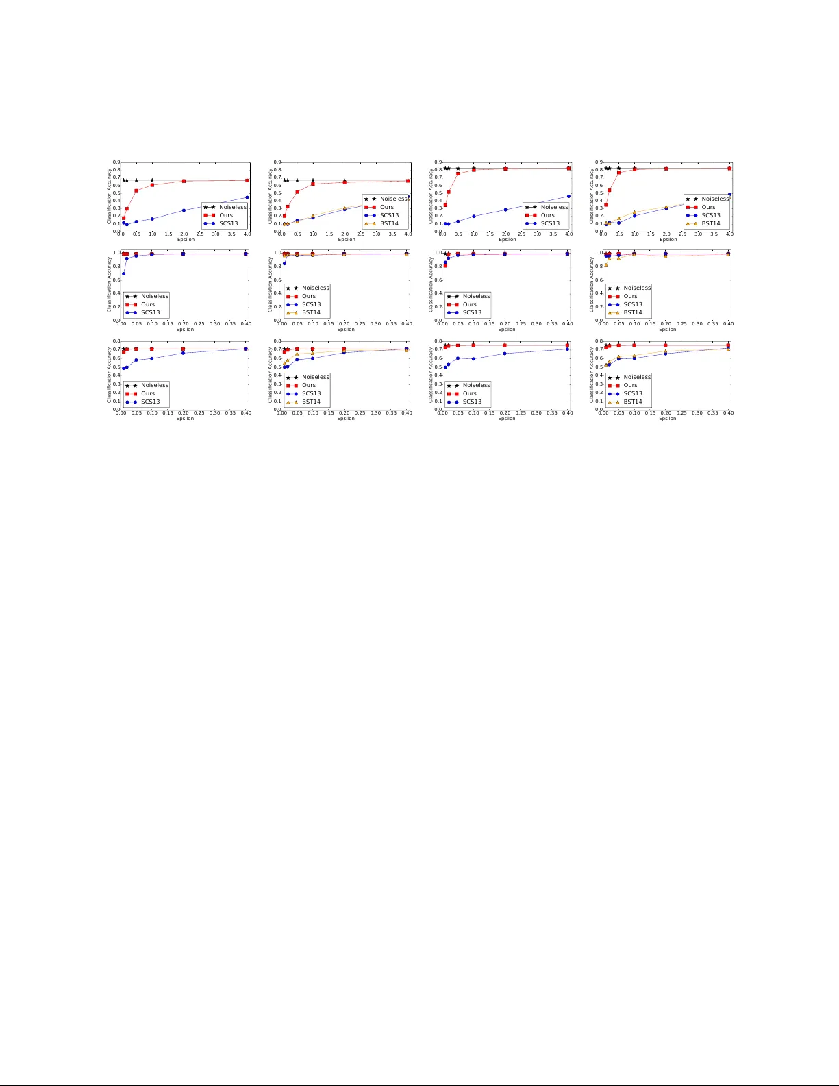
Bolt -on Di ﬀ erential Priv acy f or Scalable S tochastic Gradient Descent -based Analytics Xi W u 1 * Fengan Li 1 * Arun K umar 2 Kamalika Chaudhuri 2 Somesh Jha 3 J e ﬀ rey Na ughton 1 * 1 Google 2 University of C alifornia, San Diego 3 University of W isconsin-Madison 1 { wuxi, feng anl, naughton } @g oogle.com, 2 { arunkk, kamalika } @eng.ucsd.edu, 3 jha@cs.wisc.edu March 24, 2017 Abstract While signiﬁcant progress has been made separately on anal ytics systems for scalable stochastic gra- dient descent (SGD) and priva te SGD, none of the major scalable analytics frameworks ha ve incorpora ted di ﬀ erentiall y private SGD. There are two inter -related issues for this disconnect between research and practice: (1) low model accuracy due to added noise to guarantee privacy , and (2) high development and runtime overhead of the priv ate algorithms. This paper takes a ﬁrst step to remedy this disconnect and proposes a private SGD al gorithm to address both issues in an integrated manner . In contrast to the white- box approach adopted by previous work, we revisit and use the classical technique of output perturbation to devise a novel “bolt -on ” approach to private SGD. While our approach trivially addresses (2), it makes (1) ev en more challenging. W e address this challenge by providing a nov el analysis of the L 2 -sensitivity of SGD, which allows, under the same privacy guarantees, better converg ence of SGD when only a constant number of passes can be made over the data. W e integrate our algorithm, as well as other state-of -the- art di ﬀ erentiall y private SGD, into Bismarck , a popular scalable SGD-based analytics system on top of an RDBMS. Extensive experiments show that our alg orithm can be easily integra ted, incurs virtually no ov erhead, scales w ell, and most importantly , yields substantially better (up to 4X) test accuracy than the state-of -the-art al gorithms on man y real datasets. 1 Introduction The past decade has seen signiﬁcant interest from both the data management industry and academia in integrating machine learning (ML) algorithms into scalable data processing systems such as RDBMSs [ 23 , 19 ], Hadoop [ 1 ], and Spark [ 2 ]. In many data-driven applications such as personalized medicine, ﬁnance, web search, and social networks, there is also a growing concern about the privacy of individuals. T o this end, di ﬀ erential privacy , a cryptographically motivated notion, has emerged as the gold standard for protecting data privacy . Di ﬀ erentially private ML has been extensivel y studied by researchers from the database, ML, and theoretical computer science comm unities [ 10 , 13 , 15 , 25 , 27 , 36 , 37 ]. In this work, w e study di ﬀ erential privacy for stochastic gradient descent (SGD) , which has become the optimization algorithm of choice in many scalable ML systems, especially in-RDBMS analytics systems. * W ork done while at UW -Madison. 1 For example, Bismarck [ 19 ] o ﬀ ers a highly e ﬃ cient in-RDBMS implementation of SGD to provide a single framewor k to implement many convex analysis-based ML techniques. Thus, creating a private version of SGD would a utomatically provide priv ate v ersions of all these ML techniques. While previous work has separately studied in-RDBMS SGD and di ﬀ erentially private SGD, our con- versations with dev elopers at several database companies revealed that none of the major in-RDBMS ML tools have incorporated di ﬀ erentially private SGD. There are two inter -related reasons for this disconnect between research and practice: (1) low model accuracy due to the noise added to guarantee privacy , and (2) high development and runtime overhead of the private algorithms. One might expect tha t more sophis- ticated private algorithms might be needed to address issue (1) but then again, such alg orithms might in turn exacerbate issue (2)! T o understand these issues better , we integra te two state-of -the-art di ﬀ erentially priv ate SGD al gorithms – Song, Chaudhuri and Sarwate (SCS13 [ 35 ]) and Bassily , Smith and Thakurta (BST14 [ 10 ]) – into the in- RDBMS SGD architecture of Bismar ck . SCS13 adds noise at each iteration of SGD, enough to make the iterate di ﬀ erentiall y private. BST14 reduces the amount of noise per iteration by subsampling and can guarantee optimal converg ence using O ( m ) passes ov er the data (where m is the training set size); howev er , in many real applications, w e can only a ﬀ ord a constant number of passes, and hence, we derive and implemen t a version for O (1) passes. Empirically , we ﬁnd that both algorithms su ﬀ er from both issues (1) and (2): their accuracy is much worse than the accuracy of non-private SGD, while their “white box” paradigm requires deep code changes that require modifying the gradient update steps of SGD in order to inject noise. In turn, these changes for repea ted noise sampling lead to a signiﬁcant runtime ov erhead. In this paper , we take a ﬁrst step towards mitigating both issues in an integra ted manner . In contrast to the white box approach of prior work, we consider a new approach to di ﬀ erentially priva te SGD in which we treat the SGD implementation as a “black box” and inject noise only at the end . In order to make this bolt - on approach feasible, we revisit and use the classical technique of output perturbation [ 16 ]. An immediate consequence is that our approach can be trivially integrated into any scalable SGD system, including in- RDBMS analytics systems such as Bismar ck , with no changes to the internal code. Our approach also incurs virtually no runtime ov erhead and preserves the scalability of the existing system. While output perturbation obviously addresses the runtime and integration challenge, it is unclear what its e ﬀ ect is on model accuracy . In this work, we provide a novel analysis that leads to an output perturbation procedure with higher model accuracy than the state-of -the-art priv ate SGD alg orithms. The essence of our solution is a new bound on the L 2 -sensitivity of SGD which allows, under the same privacy guarantees, better converg ence of SGD when only a constant number of passes over the data can be made. As a result , our algorithm produces priva te models that are signiﬁcantly more accurate than both SCS13 and BST14 for practical problems. Overall, this paper makes the following con tributions: • W e propose a novel bolt -on di ﬀ erentially private al gorithm for SGD based on output perturbation. An immediate consequence of our approach is that our algorithm directly inherits many desirable properties of SGD, while allowing easy integration into existing scalable SGD-based analytics sys- tems. • W e provide a novel analysis of the L 2 -sensitivity of SGD that leads to an output perturbation proce- dure with higher model accuracy than the state-of -the- art private SGD algorithms. Importantly , our analysis allows better conv ergence when one can only a ﬀ ord running a constant number of passes over the data, which is the typical situation in practice. K ey to our analysis is the use of the well-known expansion properties of gradient opera tors [ 29 , 31 ]. • W e integrate our private SGD algorithms, SCS13, and BST14 into Bismarck and conduct a compre- hensive empirical evaluation. W e explain how our algorithms can be easily integrated with little devel opment e ﬀ ort. Using several real datasets, w e demonstrate tha t our algorithms run signiﬁcantly faster , scale well, and yield substantially better test accuracy (up to 4X) than SCS13 or BST14 for the same settings. The rest of this paper is organized as foll ows: In Section 2 we present preliminaries. In Section 3 , we present our priva te SGD algorithms and analyze their privacy and conv ergence guarantees. Along 2 the wa y , we extend our main algorithms in various ways to incorporate common practices of SGD. W e then perform a comprehensive em pirical study in Section 4 to demonstrate that our algorithms satisfy key desired properties for in-RDBMS analytics: ease of integration, low runtime overhead, good scalability , and high accuracy . W e provide more remar ks on related theoretical w ork in Section 5 and conclude with future directions in Section 6 . 2 Preliminaries This section reviews important deﬁnitions and existing resul ts. Machine Learning and Con vex ERM . Focusing on supervised learning, w e ha ve a sample space Z = X × Y , where X is a space of feature vectors and Y is a label space. W e also have an ordered training set (( x i , y i )) m i =1 . Let W ⊆ R d be a hypothesis space equipped with the standard inner product and 2-norm k·k . W e are given a loss function  : W × Z 7→ R which measures the how w ell a w classiﬁes an example ( x, y ) ∈ Z , so that giv en a hypothesis w ∈ W and a sample ( x , y ) ∈ Z , we hav e a loss  ( w , ( x , y )). Our goal is to minimize the empirical risk over the training set S (i.e., the empirical risk minimization, or ERM), deﬁned as L S ( w ) = 1 m P m i =1  ( w, ( x i , y i )). Fixing S ,  i ( w ) =  ( w, ( x i , y i )) is a function of w . In both in-RDBMS and priva te learning, convex ERM problems are common, where every  i is convex . W e start by deﬁning some basic properties of loss functions that will be needed later to present our anal ysis. Deﬁnition 1. Let f : W 7→ R be a function: • f is convex if for any u , v ∈ W , f ( u ) ≥ f ( v ) + h∇ f ( v ) , u − v i • f is L -Lipschitz if for any u , v ∈ W , k f ( u ) − f ( v ) k ≤ L k u − v k • f is γ -strongly convex if f ( u ) ≥ f ( v ) + h∇ f ( v ) , u − v i + γ 2 k u − v k 2 • f is β -smooth if k∇ f ( u ) − ∇ f ( v ) k ≤ β k u − v k Example: Logistic Regression . The above three parameters ( L , γ , and β ) are derived by analyzing the loss function. W e give an example using the popular L 2 -regularized logistic regression model with the L 2 regularization parameter λ . This derivation is standard in the optimization literature (e.g., see [ 11 ]). W e assume some preprocessing that normalizes each fea ture vector , i.e., each k x k ≤ 1 (this assumption is common for analyzing private optimization [ 10 , 13 , 35 ]. In fact , such preprocessing are also common for general machine learning problems [ 6 ], not just private ones). Recall now that for L 2 -regularized l ogistic regression the loss function on an example ( x, y ) with y ∈ {± 1 } ) is deﬁned as follows:  ( w, ( x , y )) = ln  1 + exp( − y h w, x i )  + λ 2 k w k 2 (1) Fixing λ ≥ 0, w e can obtain L , γ , and β by l ooking at the expression for the gradient ( ∇  ( w )) and the Hessian ( H (  ( w ))). L is chosen as a tight upper bound on k∇  ( w ) k , β is chosen as a tight upper bound on k H (  ( w )) k , and γ is chosen such that H (  ( w ))  γ I , i.e., H (  ( w )) − γ I is positive semideﬁnite). Now there are two cases depending on whether λ > 0 or not. If λ = 0 w e do not hav e strong conv exity (in this case it is only convex), and we hav e L = β = 1 and γ = 0. If λ > 0, we need to assume a bound on the norm of the hypothesis w . (which can be achieved by rescaling). In particular , suppose k w k ≤ R , then together with k x k ≤ 1, we can deduce that L = 1 + λR , β = 1 + λ , and γ = λ . W e remark that these are indeed standard val ues in the literature f or L 2 -regularized logistic loss [ 11 ]. The above assumptions and deriv ation are common in the optimization literature [ 11 , 12 ]. In some ML models,  is not di ﬀ erentiable, e.g., the hinge loss for the linear SVM [ 4 ]. The standard approach in this 3 case is to approximate it with a di ﬀ erentiable and smooth function. For example, for the hinge loss, there is a body of work on the so-called Huber SVM [ 4 ]. In this paper , we focus primarily on logistic regression as our example but w e also discuss the Huber SVM and present experiments for it in the appendix. Stochastic Gradient Descent . SGD is a simple but popular optimization algorithm that performs many incremental gradient updates instead of computing the full gradient of L S . At step t , given w t and a random example ( x t , y t ), SGD’ s update rule is as follows: w t +1 = G  t ,η t ( w t ) = w t − η t  0 t ( w t ) (2) where  t ( · ) =  ( · ; ( x t , y t )) is the loss function and η t ∈ R is a parameter called the learning rate , or step size . W e will denote G  t ,η t as G t . A form of SGD that is commonly used in practice is perm utation-based SGD (PSGD): ﬁrst sample a random perm utation τ of [ m ] ( m is the size of the training set S ), and then repea tedly apply ( 2 ) by cycling through S according to τ . In particular , if we cycle through the dataset k times, it is called k -pass PSGD. W e now deﬁne two important properties of gradient updates that are needed to understand the anal- ysis of SGD’ s converg ence in general, as well as our new technical results on di ﬀ erentially private SGD: expansiveness and boundedness . Speciﬁcall y , we use these deﬁnitions to introd uce a simple but important recent optimization-theoretical result on SGD’ s behavior by [ 21 ] that we adapt and apply to our problem setting. Intuitively , expansiv eness tells us how much G can expand or contract the distance between two hypotheses, while boundedness tells us how much G modiﬁes a given hypothesis. W e now provide the formal deﬁnitions (due to [ 29 , 31 ]). Deﬁnition 2 (Expansiveness) . Let G : W 7→ W be an operator that maps a hypothesis to another hypothesis. G is said to be ρ -expansive if sup w,w 0 k G ( w ) − G ( w 0 ) k k w − w 0 k ≤ ρ. Deﬁnition 3 (Boundedness) . Let G : W 7→ W be an operator that maps a hypothesis to another hypothesis. G is said to be σ -bounded if sup w ∈W k G ( w ) − w k ≤ σ . Lemma 1 (Expansiveness ([ 29 , 31 ])) . Assume that  is β -smooth. Then, the following hold. 1. If  is convex, then for any η ≤ 2 / β , G  ,η is 1 -expansive. 2. If  is γ -strongly convex, then for η ≤ 2 β + γ , G  ,η is (1 − 2 η β γ β + γ ) -expansive. In particular we use the foll owing simpliﬁcation d ue to [ 21 ]. Lemma 2 ([ 21 ]) . Suppose that  is β -smooth and γ -strongly convex. If η ≤ 1 β , then G  ,η is (1 − η γ ) -expansive. Lemma 3 (Boundedness) . Assume that  is L -Lipschitz. Then the gradient update G  ,η is ( η L ) -bounded. W e are ready to describe a key quantity studied in this paper . Deﬁnition 4 ( δ t ) . Let w 0 , w 1 , . . . , w T , and w 0 0 , w 0 1 , . . . , w 0 T be two sequences in W . W e deﬁne δ t as k w t − w 0 t k . The foll owing lemma by Hard t, Recht and Sing er [ 21 ] bounds δ t using expansiv eness and boundedness properties (Lemma 1 and 3 ). Lemma 4 ( Growth Recursion [ 21 ]) . Fix any two sequences of updates G 1 , . . . , G T and G 0 1 , . . . , G 0 T . Let w 0 = w 0 0 and w t = G t ( w t − 1 ) and w 0 t = G 0 t ( w 0 t − 1 ) for t = 1 , 2 , . . . , T . Then δ 0 = 0 , and for 0 < t ≤ T δ t ≤                ρδ t − 1 G t = G 0 t is ρ -expansive. min( ρ, 1) δ t − 1 + 2 σ t G t and G 0 t are σ t -bounded, G t is ρ -expansive. 4 Essentially , Lemma 4 is used as a tool to prove “ averag e-case stability” of standard SGD in [ 21 ]. W e adapt and apply this result to our problem setting and devise new di ﬀ erentiall y private SGD algorithms. 1 The applica tion is non-trivial beca use of our unique desiderata but we achieve it by lev eraging other recent important optimization-theoretical results by [ 34 ] on the converg ence of PSGD. Overall, by synthesizing and building on these recent resul ts, we are able to prov e the converg ence of our priva te SGD algorithms as well. Di ﬀ erential Privacy . W e sa y that two datasets S , S 0 are neighboring , denoted by S ∼ S 0 , if they di ﬀ er on a single individual’ s private v al ue. Recall the following deﬁnition: Deﬁnition 5 (( ε, δ )-di ﬀ erential privacy) . A (randomized) algorithm A is said to be ( ε, δ )-di ﬀ erentially priv ate if for any neighboring datasets S , S 0 , and any event E ⊆ Range( A ) , Pr[ A ( S ) ∈ E ] ≤ e ε Pr[ A ( S 0 ) ∈ E ] + δ. In particular , if δ = 0, we will use ε -di ﬀ erential privacy instead of ( ε , 0)-di ﬀ erential privacy . A basic paradigm to achieve ε -di ﬀ erential priv acy is to examine a query’ s L 2 -sensitivity , Deﬁnition 6 ( L 2 -sensitivity) . Let f be a deterministic query that maps a dataset to a vector in R d . The L 2 - sensitivity of f is deﬁned to be ∆ 2 ( f ) = max S ∼ S 0 k f ( S ) − f ( S 0 ) k . The following theorem rela tes ε -di ﬀ erential privacy and L 2 -sensitivity . Theorem 1 ([ 16 ]) . Let f be a deterministic query that maps a database to a vector in R d . Then publishing f ( D ) + κ where κ is sampled from the distribution with density p ( κ ) ∝ exp − ε k κ k ∆ 2 ( f ) ! (3) ensures ε -di ﬀ erential privacy . For the interested reader , we provide a detailed algorithm in Appendix E for how to sample from the above distribution. Importantly , the L 2 -norm of the noise vector , k κ k , is distributed according to the Gamma distribution Γ ( d , ∆ 2 ( f ) / ε ) . W e have the f ollowing fact about Gamma distributions: Theorem 2 ([ 13 ]) . F or the noise vector κ , we have that with probability at least 1 − γ , k κ k ≤ d ln( d / γ ) ∆ 2 ( f ) ε . Note that the noise depends linearithmically on d . This could destroy utility (lower accuracy dramati- cally) if d is high. But there are standard techniques to mitigate this issue that are commonly used in private SGD literature (we discuss more in Section 4.3 ). By switching to Gaussian noise, we obtain ( ε , δ )-di ﬀ erential privacy . Theorem 3 ([ 17 ]) . Let f be a deterministic query that maps a database to a vector in R d . Let ε ∈ (0 , 1) be arbitrary . F or c 2 > 2 ln(1 . 25 / δ ) , adding Gaussian noise sampled according to N (0 , σ 2 ); σ ≥ c ∆ 2 ( f ) ε , c 2 > 2 ln  1 . 25 δ  (4) ensures ( ε, δ ) -di ﬀ er entially privacy . For Gaussian noise, the dependency on d is √ d , instead of d ln d . Random Projection . Known conv ergence results of private SGD (in fact private ERM in general) have a poor dependencies on the dimension d . T o handle high dimensions, a useful technique is random projec- tion [ 7 ]. That is, we sample a random linear transformation T from certain distributions and apply T to each feature point x in the training set, so x is transformed to T x . Note that after this transformation two neighboring datasets (datasets di ﬀ ering at one data point) remain neighboring, so random projection does 1 Interestingly , di ﬀ erential privacy can be view ed as notion of “worst -case stability . ” Thus we o ﬀ er “worst -case stability . ” 5 not a ﬀ ect our privacy analysis. Further , the theory of random projection will tell “what low dimension ” to project to so that “ approximate utility will be preserved. ” (in our MNIST experiments the accuracy gap between original and projected dimension is very small). Thus, for problems with higher dimensions, w e invoke the random projection to “l ower” the dimension to achiev e small noise and thus better utility , while preserving privacy . In our experimental study we appl y random projection to one of our datasets (MNIST). 3 Priv ate SGD W e present our di ﬀ erentiall y private PSGD alg orithms and analyze their privacy and conv ergence guaran- tees. Speciﬁcally , we present a new analysis of the output perturbation method for PSGD. Our new analysis shows that very little noise is needed to achieve di ﬀ erential privacy . In fact, the resulting private algorithms hav e g ood conv ergence rates with even one pass ov er the data. Since output perturba tion also uses standard PSGD algorithm as a black -box, this makes our algorithms attractiv e for in-RDBMS scenarios. This section is structured accordingly in two parts. In Section 3.1 we give two main di ﬀ erentially private algorithms for convex and strongly conv ex optimization. In Section 3.2 we ﬁrst prove that these two algo- rithms are di ﬀ erentially priv ate (Section 3.2.1 and 3.2.2 ), then extend them in v arious wa ys (Section 3.2.3 ), and ﬁnally prov e their conv ergence (Section 3.2.4 ). 3.1 Algorithms As we mentioned before, our di ﬀ erentially priva te PSGD algorithms uses one of the most basic paradigms for achieving di ﬀ erential privacy – the output perturbation method [ 16 ] based on L 2 -sensitivity (Deﬁni- tion 6 ). Speciﬁcally , our algorithms are “instantiations” of the output perturbation method where the L 2 -sensitivity parameter ∆ 2 is derived using our new analysis. T o describe the algorithms, we assume a standard permutation-based SGD procedure (denoted as PSGD ) which can be invoked as a black -box. T o facilitate the presenta tion, T able 1 summarizes the parameters. Symbol Meaning λ L 2 -regularization parameter . L Lipschitz constant. γ S trong conv exity . β Smoothness. ε, δ Privacy parameters. η t Learning rate or step size at itera tion t . W A conv ex set that forms the h ypothesis space. R Radius of the hypothesis space W . k Number of passes through the data. b Mini-ba tch size of SGD. m Size of the training set S . T able 1: Notations . Algorithms 1 and 2 give our priv ate SGD alg orithms for conv ex and strongly con vex cases, respectivel y . A key di ﬀ erence between these two algorithms is at line 3 where di ﬀ erent L 2 -sensitivities are used to sample the noise κ . Note that di ﬀ erent learning rates are used: In the conv ex case, a constant rate is used, while a decreasing rate 1 γ t is used in the strongly conv ex case. Finally , note that the standard PSGD is in voked as a black box at line 2 . 6 Algorithm 1 Priv ate Con vex P ermutation-based SGD Require:  ( · , z ) is conv ex for ev ery z , η ≤ 2 / β . Input: Da ta S , parameters k , η , ε 1: function PrivateC onvexPSGD ( S , k , ε , η ) 2: w ← PSGD ( S ) with k passes and η t = η 3: ∆ 2 ← 2 k Lη 4: Sample noise v ector κ according to ( 3 ). 5: return w + κ Algorithm 2 Priv ate S trongly Con vex P ermutation-based SGD Require:  ( · , z ) is γ -strongly conv ex for ev ery z Input: Da ta S , parameters k , ε 1: function PrivateStr onglyConvexPSGD ( S , k , ε ) 2: w ← PSGD ( S ) with k passes and η t = min( 1 β , 1 γ t ) 3: ∆ 2 ← 2 L γ m 4: Sample noise v ector κ according to ( 3 ). 5: return w + κ 3.2 Analysis In this section we inv estigate privacy and conv ergence guarantees of Algorithms 1 and 2 . Along the wa y , we also describe extensions to accommodate common practices in running SGD. Most proofs in this section are deferred to the appendix. Overview of the Analysis and K ey Observations. For priv acy , let A ( r ; S ) denote a randomized non-priva te algorithm where r denotes the randomness (e.g., random permutations sampled by SGD) and S denotes the input training set. T o bound L 2 -sensitivity we want to bound max r ,r 0 k A ( r ; S ) − A ( r 0 ; S 0 ) k on a pair of neighboring datasets S , S 0 , where r , r 0 can be di ﬀ erent randomness sequences of A in general. This can be complicated since A ( r ; · ) and A ( r 0 ; · ) may access the da ta in vastl y di ﬀ erent pa tterns. Our key observation is that for non-adaptive randomized algorithms, it su ﬃ ces to consider randomness sequences one at a time , and thus bound max r k A ( r ; S ) − A ( r ; S 0 ) k . This in turn allows us to obtain a small upper bound of the L 2 -sensitivity of SGD by combining the expansion properties of gr adient operators and the fact that one will onl y access once the di ﬀ ering da ta point betw een S and S 0 for each pass over the data, if r is a random permutation. Finally for conv ergence, while using permutation beneﬁts our privacy proof, the converg ence behavior of permutation-based SGD is poor ly understood in theory . Fortunately , based on very recent adv ances by Shamir [ 34 ] on the sampling-without -replacement SGD, we prove convergence of our private SGD algo- rithms even with onl y one pass over the data. Randomness One at a T ime. Consider the following deﬁnition, Deﬁnition 7 (Non- Adaptive Al gorithms) . A randomized algorithm A is non- adaptive if its random choices do not depend on the input data values. PSGD is clearly non-adaptive as a single random permutation is sampled at the very beginning of the algorithm. Another common SGD variant, where one independently and uniformly samples i t ∼ [ m ] at iteration t and picks the i t -th data point, is also non-adaptive. In fact, more modern SGD variants, such as Stochastic V ariance Reduced Gradient (SVRG [ 26 ]) and Stochastic A verag e Gradient (SA G [ 32 ]), are non- adaptive as w ell. Now we ha v e the following lemma f or non-adaptiv e alg orithms and di ﬀ erential priv acy . Lemma 5. Let A ( r ; S ) be a non-adaptive randomized algorithm where r denotes the randomness of the algorithm and S denotes the dataset A works on. Suppose that sup S ∼ S 0 sup r k A ( r ; S ) − A ( r ; S 0 ) k ≤ ∆ . 7 Then publishing A ( r ; S ) + κ where κ is sampled with density p ( κ ) ∝ exp  − ε k κ k 2 ∆  ensures ε -di ﬀ erential privacy . Proof. Let e A denote the private version of A . e A has two parts of randomness: One part is r , which is used to compute A ( r ; S ); the second part is κ , which is used for perturbation (i.e. A ( r ; S ) + κ ). Let R be the random variable corresponding to the randomness of A . Note that R does not depend on the input training set. Thus for an y event E , Pr[ e A (( r , κ ); S ) ∈ E ] = X r Pr[ R = r ] · Pr κ [ A (( r , κ ); S ) ∈ E | R = r ] . (5) Denote Pr κ [ A (( r , κ ); S ) ∈ E | R = r ] by p κ ( A r ( S ) ∈ E ). Then similarly for S 0 we ha ve that Pr[ e A (( r , κ ); S 0 ) ∈ E ] = X r Pr[ R = r ] · p κ ( A r ( S 0 ) ∈ E ) . (6) Compare ( 5 ) and ( 6 ) term by term (for every r ): the lemma then follows as we calibrate the noise κ so that p κ ( A r ( S ) ∈ E ) ≤ e ε p κ ( A r ( S 0 ) ∈ E ). From now on we denote PSGD by A . With the notations in Deﬁnition 4 , our next goal is thus to bound sup S ∼ S 0 sup r δ T . In the next two sections we bound this quantity for convex and strongly conv ex optimiza- tion, respectivel y . 3.2.1 Conv ex Optimization In this section we prove privacy guarantee when  ( · , z ) is convex. Recall that for general convex optimiza- tion, we ha ve 1-expansiv eness by Lemma 1.1 . W e thus have the f ollowing lemma that bounds δ T . Lemma 6. C onsider k -passes PSGD for L -Lipschitz, convex and β -smooth optimization where η t ≤ 2 β for t = 1 , . . . , T . Let S , S i be any neighboring datasets. Let r be a random permutation of [ m ] . Suppose that r ( i ) = i ∗ . Let T = k m , then δ T ≤ 2 L P k − 1 j =0 η i ∗ + j m . W e immediately hav e the following corollary on L 2 -sensitivity with constant step size, Corollary 1 (Constant S tep Size) . Consider k -passes PSGD for L -Lipschitz, convex and β -smooth op timization. Suppose further that we have constant learning rate η 1 = η 2 = · · · = η T = η ≤ 2 β . Then sup S ∼ S 0 sup r δ T ≤ 2 k Lη . This directly yields the f ollowing theorem, Theorem 4. Algorithm 1 is ε -di ﬀ er entially private. W e now give L 2 -sensitivity results for two di ﬀ erent choices of step sizes, which are also common for conv ex optimization. Corollary 2 ( Decreasing Step Size) . Let c ∈ [0 , 1) be some constant. Consider k -passes PS GD for L -Lipschitz, convex and β -smooth optimization. Suppose further that we take decreasing step size η t = 2 β ( t + m c ) where m is the training set size. Then sup S ∼ S 0 sup r δ T = 4 L β  1 m c + ln k m  . Corollary 3 ( Square-Root S tep Size) . Let c ∈ [0 , 1) be some constant. C onsider k -passes PSGD for L -Lipschitz, convex and β -smooth optimization. Suppose further that we take square-root step size η t = 2 β ( √ t + m c ) . Then sup S ∼ S 0 sup r δ T ≤ 4 L β         k − 1 X j =0 1 p j m + 1 + m c         = O       L β       1 m c + min       k m c , r k m                   . 8 Remark on Constant S tep Size . In Lemma 1 the step size is named “constant” for the SGD. However , one should note that Constant step size for SGD can depend on the size of the training set, and in particular can vanish to zero as training set size m increases. For example, a typical setting of step size is 1 √ m (In fact, in typical converg ence results of SGD, see, for example in [ 12 , 28 ], the constant step size η is set to 1 / T O (1) where T is the total number of iter ations). This, in particular , implies a sensitivity O ( k η ) = O ( k / √ m ), which vanishes to 0 as m grows to inﬁnity . 3.2.2 Strongly C onv ex Optimization Now we consider the case where  ( · , z ) is γ -strongly convex. In this case the sensitivity is smaller because the gradient operators are ρ -expansiv e for ρ < 1 so in particular they become contractions. W e have the following lemmas. Lemma 7 (Constant Step Size) . Consider PS GD for L -Lipschitz, γ -strongly convex and β -smooth optimization with constant step sizes η ≤ 1 β . Let k be the number of passes. Let S , S 0 be two neighboring datasets di ﬀ ering at the i -th data point. Let r be a random permutation of [ m ] . Suppose that r ( i ) = i ∗ . Let T = k m , then δ T ≤ 2 Lη P k − 1 j =0 (1 − η γ ) ( k − j ) m − i ∗ . In particular , sup S ∼ S 0 sup r δ T ≤ 2 η L 1 − (1 − η γ ) m . Lemma 8 ( Decreasing Step Size) . Consider k -passes PSGD for L -Lipschitz, γ -strongly convex and β -smooth op- timization. Suppose further that we use decreasing step length: η t = min( 1 γ t , 1 β ) . Let S , S 0 be two neighboring datasets di ﬀ ering at the i -th data point. Let r be a r andom permutation of [ m ] . Suppose that r ( i ) = i ∗ . Let T = k m , then sup S ∼ S 0 sup r δ T ≤ 2 L γ m . In particular , Lemma 8 yiel ds the following theorem, Theorem 5. Algorithm 2 is ε -di ﬀ er entially private. One should contrast this theorem with Theorem 4 : In the conv ex case we bound L 2 -sensitivity by 2 k Lη , while in the strongly conv ex case w e bound it by 2 L/ γ m. 3.2.3 Extensions In this section we extend our main argument in sev eral wa ys: ( ε , δ )-di ﬀ erential privacy , mini-batching, model av eraging, fresh permutation at each pass, and ﬁnally constrained optimization. These extensions can be easily incorporated to standard PSGD algorithm, as well as our private alg orithms 1 and 2 , and are used in our empirical study later . ( ε, δ ) -Di ﬀ erential Privacy . W e can also obtain ( ε, δ )-di ﬀ eren tial privacy easily using Gaussian noise (see Theorem 3 ). Lemma 9. Let A ( r ; S ) be a non-adaptive randomized algorithm where r denotes the randomness of the algorithm and S denote the dataset. Suppose that sup S ∼ S 0 sup r k A ( r ; S ) − A ( r ; S 0 ) k ≤ ∆ . Then for any ε ∈ (0 , 1) , publishing A ( r ; S ) + κ where each component of κ is sampled using ( 4 ) ensures ( ε , δ ) - di ﬀ erential privacy . In particular , combining this with our L 2 -sensitivity results, w e get the foll owing two theorems, Theorem 6 (Conv ex and Constant Step) . Algorithm 1 is ( ε, δ ) -di ﬀ er entially private if each component of κ at line 3 is sampled according to equation ( 4 ). 9 Theorem 7 (Strongly Conv ex and Decreasing Step) . Algorithm 2 is ( ε , δ ) -di ﬀ er entially private if each compo- nent of κ at line 3 is sampled according to equation ( 4 ). Mini-batching . A popular way to do SGD is that at each step, instead of sampling a single data point z t and do gradient update w .r .t. it, we r andomly sample a ba tch B ⊆ [ m ] of size b , and do w t = w t − 1 − η t 1 b        X i ∈ B  0 i ( w t − 1 )        = 1 b X i ∈ B G i ( w t − 1 ) . For permuta tion SGD, a natural way to employ mini-batch is to partition the m data points into mini- batches of size b (for simplicity let us assume that b divides m ), and do gradient updates with respect to each chunk. In this case, we notice tha t mini-batch indeed im proves the sensitivity by a factor of b . In fact, let us consider neighboring datasets S , S 0 , and a t step t , w e hav e batches B, B 0 that di ﬀ er in at most one data point. Without loss of generality , let us consider the case where B, B 0 di ﬀ er at one data point, then on S we hav e w t = 1 b P i ∈ B G i ( w t − 1 ) , and on S 0 we ha ve w 0 t = 1 b P i ∈ B G 0 i ( w 0 t − 1 ) , and so δ t =        1 b X i ∈ B G i ( w t − 1 ) − G 0 i ( w 0 t − 1 )        ≤ 1 b B X i =1 k G i ( w t − 1 ) − G 0 i ( w 0 t − 1 ) k . W e note that for all i except one in B , G i = G 0 i , and so by the Growth Recursion Lemma 4 , k G i ( w t − 1 ) − G 0 i ( w 0 t − 1 ) k ≤ ρδ t − 1 if G i is ρ -expansive, and for the di ﬀ ering index i ∗ , k G i ∗ ( w t − 1 ) − G 0 i ∗ ( w 0 t − 1 ) k ≤ min( ρ, 1) δ t − 1 + 2 σ t . Therefore, for a uniform bound ρ t on expansiveness and σ t on boundedness (for all i ∈ B , which is the case in our analysis), we have that δ t ≤ ρ t δ t − 1 + 2 σ t b . This implies a factor b improv ement for all our sensitivity bounds. Model A ver aging . Model av eraging is a popular technique for SGD. F or example, giv en itera tes w 1 , . . . , w T , a common way to do model av eraging is either to output 1 T P T t =1 w t or output the av erage of the last log T iterates. W e show that model averaging will not a ﬀ ect our sensitivity result, and in fact it will give a constant -factor improvement when earlier iterates have smaller sensitivities. W e have the following lemma. Lemma 10 (Model A veraging) . Suppose that instead of returning w T at the end of the optimization, we return an averaged model ¯ w = P T t =1 α t w t , where α t is a sequence of coe ﬃ cients that only depend on t , T . Then, sup S ∼ S 0 sup r k ¯ w − ¯ w 0 k ≤ T X t =1 α t k w t − w 0 t k = T X t =1 α t δ t . In particular , we notice that the δ t ’ s we derived before are non-decreasing, so the sensitivity is bounded by ( P T t =1 α t ) δ T . Fresh P erm utation at Each P ass . W e note tha t our analysis extends verbatim to the case where in each pass a new permutation is sam pled, as our analysis applies to any ﬁxed perm utation. Constrained Optimization . Until now , our SGD algorithm is for unconstrained optimization. That is, the hypothesis space W is the entire R d . Our results easily extend to constrained optimization where the hypothesis space W is a convex set C . That is, our goal is to compute min w ∈C L S ( w ). In this case, we change the original gradient update rule 2 to the projected gr adient update rule : w t = Y C  w t − 1 − η t  0 t ( w t − 1 )  , (7) where Q C ( w ) = arg min v k v − w k is the projection of w to C . It is easy to see that our analysis carries over verbatim to the projected gr adient descent. In fact , our analysis works as l ong as the optimiza tion is carried over a Hilbert space (i.e., the k · k is induced by some inner product). The essential reason is that projection will not increase the distance ( k Q u − Q v k ≤ k u − v k ), and thus will not a ﬀ ect our sensitivity argumen t. 10 3.2.4 Conv ergence of Optimiza tion W e now bound the optimization error of our private PSGD algorithms. More speciﬁcally , we bound the excess empirical risk L S ( w ) − L ∗ S where L S ( w ) is the loss of the output w of our priva te SGD alg orithm and L ∗ S is the minim um obtained by an y w in the f easible set W . Note that in PSGD w e sample data points without replacement . While sampling without replacement beneﬁts our L 2 -sensitivity argument, its conv ergence behavior is poorly understood in theory . Our results are based on v ery recent advances by Shamir [ 34 ] on the sampling-without -replacement SGD. As in Shamir [ 34 ], w e assume that the l oss function  i takes the form of  i ( h w, x i i ) + r ( w ) where r is some ﬁxed function. Further we assume that the optimization is carried over a convex set C of radius R (i.e., k w k ≤ R for w ∈ C ). W e use projected PSGD algorithm (i.e., we use the projected gr adient update rule 7 ). Finally , R ( T ) is a regret bound if for an y w ∈ W and con vex-Lipschitz  1 , . . . ,  T , P T t =1  t ( w t ) − P T t =1  t ( w ) ≤ R ( T ) and R ( T ) is sublinear in T . W e use the following regret bound, Theorem 8 (Zinkevich [ 38 ]) . F or SGD with constant step size η 1 = η 2 = · · · = η T = η , R ( T ) is bounded by R 2 2 η + L 2 T η 2 . The following lemma is useful in bounding excess em pirical risk. Lemma 11 (Risk due to Privacy) . Consider L -Lipschitz and β -smooth optimization. Let w be the output of the non-private SGD algorithm, κ be the noise of the output perturbation, and e w = w + κ . Then L S ( w ) − L S ( e w ) ≤ L k κ k . ε -Di ﬀ erential Privacy . W e now give con verg ence result f or SGD with ε -di ﬀ erential privacy . C onvex Optimization . If  ( · , z ) is convex, w e use the following theorem from Shamir [ 34 ], Theorem 9 (Corollary 1 of Shamir [ 34 ]) . Let T ≤ m (that is we take at most 1 -pass over the data). Suppose that each iterate w t is chosen from W , and the S GD algorithm has r egret bound R ( T ) , and that sup t ,w ∈W |  t ( w ) | ≤ R , and k w k ≤ R for all w ∈ W . Finally , suppose that each loss function  t takes the form ¯  ( h w, x t i ) + r ( w ) for some L -Lipschitz ¯  ( · , x t ) and k x t k ≤ 1 , and a ﬁxed r , then E        1 T T X t =1 L S ( w t ) − L S ( w ∗ )        ≤ R ( T ) T + 2(12 + √ 2 L ) R √ m . T ogether with Theorem 8 , w e thus hav e the foll owing lemma, Lemma 12. C onsider the same settin g as in Theorem 9 , and 1 -pass PSGD optimization deﬁned according to rule ( 7 ). Suppose further that we have constant learning rate η = R L √ m . Finally , let ¯ w m be the model aver aging 1 m P T t =1 w t . Then, E [ L S ( ¯ w T ) − L ∗ S ] ≤ ( L + 2(12 + √ L )) R √ m . Now we can bound the excess em pirical risk as follows, Theorem 10 ( Conv ex and Constant Step Size) . Consider the same setting as in Lemma 12 where the step size is constant η = R L √ m . Let ˜ w = ¯ w T + κ be the result of Algorithm 1 . Then E [ L S ( ˜ w ) − L ∗ S ] ≤ ( L + (2(12 + √ L )) R √ m + 2 d LR ε √ m . Note that the term 2 d LR ε √ m corresponds to the expectation of L k κ k . Str ongly C onvex Optimization . If  ( · , z ) is γ -strongly convex, w e instead use the following theorem, 11 Theorem 11 (Theorem 3 of Shamir [ 34 ]) . Suppose W has diameter R , and L S ( · ) is γ -strongly convex on W . Assume that each loss function  t takes the for ¯  ( h w t , x t i ) + r ( w ) where k x i k ≤ 1 , r ( · ) is possibly some regularization term, and each ¯  ( · , x t ) is L -Lipschitz and β -smooth. F urthermore, suppose sup w ∈W k  0 t ( w ) k ≤ G . Then for any 1 < T ≤ m , if we run SGD for T iterations with step size η t = 1 / γ t , we have E        1 T T X t =1 L S ( w t ) − L S ( w ∗ )        ≤ c · (( L + β R ) 2 + G 2 ) log T γ T , where c is some universal positive constant. By the same argument as in the conv ex case, we ha ve, Theorem 12 ( Strongly Convex and Decreasing Step Size) . Consider the same setting as in Theorem 11 wher e the step size is η t = 1 γ t . Consider 1 -pass PSGD. Let ¯ w T be the result of model averaging and ˜ w = ¯ w T + κ be the result of output perturbation. Then E [ L S ( ˜ w ) − L S ( w ∗ )] ≤ c · (( L + β R ) 2 + G 2 ) log m γ m + 2 d G 2 εγ m . Remark . Our conv ergence results for ε -di ﬀ erential privacy is di ﬀ erent from previous work, such as BST14, which onl y give convergence for ( ε, δ )-di ﬀ erential privacy for δ > 0. In fact , BST14 relies in an essen tial w ay on the advanced composition of ( ε , δ )-di ﬀ erential privacy [ 17 ] and we are not aware its converg ence for ε - di ﬀ erential privacy . Note that ε -di ﬀ erential privacy is qualitatively di ﬀ erent from ( ε , δ )-di ﬀ erential privacy (see, for example, paragr aph 3, pp. 18 in Dwork and Roth [ 17 ], as w ell as a recent article by McSherry [ 5 ]). W e believe that our conv ergence resul ts for ε -di ﬀ erential priv acy is important in its own right. ( ε, δ ) -Di ﬀ erential Privacy . By replacing Laplace noise with Gaussian noise, w e can derive similar conver - gence resul ts of our algorithms f or ( ε, δ )-di ﬀ eren tial privacy f or 1-pass SGD. It is now instructive to compare our conv ergence results with BST14 for constant number of passes. In particular , by plugging in di ﬀ eren t parameters into the analysis of BST14 (in particular , Lemma 2.5 and Lemma 2.6 in BST14) one can derive v ariants of their resul ts for constant n umber of passes. The foll owing table compares the conv ergence in terms of the dependencies on the number of training points m , and the number of dimensions d . Ours BST14 Conv ex O  √ d √ m  O  √ d (log 3 / 2 m ) √ m  Strongly C onv ex O  √ d log m m  O  d log 2 m m  T able 2: Converg ence for ( ε, δ )-DP and constant number of passes . In particular , in the convex case our convergence is better with a log 3 / 2 m factor , and in the strongly conv ex case ours is better with a √ d log m factor . These logarithmic factors are inherent in BST14 due to its dependence on some optimization results (Lemma 2.5, 2.6 in their paper), which we do not rely on . Therefore, this comparison gives theoretical evidence that our algorithms converge better for constant number passes . On the other hand, these logarithmic factors become irrelevant for BST14 with m passes, as the denominator becomes m in the conv ex case, and becomes m 2 in the strongly case, giving better dependence on m there. 4 Implementa tion and Ev alua tion In this section, we present a comprehensive em pirical study comparing three alternativ es for priva te SGD: two previously proposed state-of -the-art private SGD alg orithms, SCS13 [ 35 ] and BST14 [ 10 ], and our algorithms which are instantia tions of the output perturbation method with our new analysis. Our goal is to answer four main questions associated with the key desiderata of in-RDBMS implemen- tations of priv ate SGD, viz., ease of integration, run time overhead, scalability , and accuracy: 12 1. What is the e ﬀ ort to integrate each algorithm into an in-RDBMS analytics system? 2. What is the runtime overhead and scalability of the private SGD implementations? 3. How does the test accuracy of our algorithms compare to S C S13 and BST14? 4. How do various parameters a ﬀ ect the test accuracy? As a summary , our main ﬁndings are the following: (i) Our SGD algorithms require almost no changes to Bismarck , while both SCS13 and BST14 require deeper code changes. (ii) Our algorithms incur virtually no runtime overhead, while SCS13 and BST14 run much slower . Our algorithms scale linearly with the dataset size. While SCS13 and BST14 also enjoy linear scalability , the runtime overhead they incur also increases linearly . (iii) Under the same di ﬀ erential privacy guarantees, our private SGD algorithms yield substantially better accuracy than SCS13 and BST14, for all datasets and settings of parameters we test. (iv) As for the e ﬀ ects of parameters, our empirical results align well with the theory . For example, as one might expect, mini-batch sizes are important for reducing privacy noise. The number of passes is more subtle. For our algorithm, if the learning task is only conv ex, more passes result in larg er noise (e.g., see Lemma 1 ), and so give rise to potentially worse test accuracy . On the other hand, if the learning task is strongly convex, the number of passes will not a ﬀ ect the noise magnitude (e.g., see Lemma 8 ). As a result, doing more passes may lead to better converg ence and thus potentially better test accuracy . Interestingly , we note that slightly enlarging mini-batch size can reduce noise very e ﬀ ectively so it is a ﬀ ordable to run our private algorithms for more passes to get better convergence in the convex case. This corroborates the results of [ 35 ] that mini-ba tches are helpful in private SGD settings. In the rest of this section we give more details of our eval uation. Our discussion is structured as follows: In Section 4.1 w e ﬁrst discuss the implemented algorithms. In particular , w e discuss how w e modify SCS13 and BST14 to make them better ﬁt into our experiments. W e also give some remarks on other relevant previous algorithms, and on parameter tuning. Then in Section 4.2 we discuss the e ﬀ ort of integrating di ﬀ erent algorithms into Bismarck . Next Section 4.3 discusses the experimental design and datasets for runtime overhead, scalability and test accuracy . Then in Section 4.4 , w e report runtime ov erhead and scalability results. W e report test accuracy results for various datasets and parameter settings, and discuss the e ﬀ ects of parameters in Section 4.5 . Finall y , we discuss the lessons we learned from our experiments 4.6 . 4.1 Implemented Al gorithms W e ﬁrst discuss im plementations of our algorithms, SCS13 and BST14. Importantly , w e extend both SCS13 and BST14 to make them better ﬁt into our experiments. Among these extensions, probably most impor - tantly , we extend BST14 to support a smaller number of iterations through the data and reduce the amount of noise needed for each iteration. Our extension makes BST14 more competitive in our experiments. Our Alg orithms . W e implement Algorithms 1 and 2 with the extensions of mini-batching and constr ained optimization (see Section 3.2.3 ). Note that Bismar ck already supports standard PSGD alg orithm with mini- batching and constr ained optimiza tion. Therefore the only change w e need to make for Algorithms 1 and 2 (note that the total number of updates is T = k m ) is the setting of L 2 -sensitivity parameter ∆ 2 at line 3 of respective al gorithms, which we divide by b if the mini-batch size is b . SCS13 [ 35 ] . W e modify [ 35 ], which originally only supports one pass through the data, to support multi- passes over the data. BST14 [ 10 ] . BST14 provides a second sol ution for priv ate SGD following the same paradigm as SCS13, but with less noise per iteration. This is achieved by ﬁrst, using a novel subsampling technique and second, relaxing the privacy guarantee to ( ε , δ )-di ﬀ eren tial privacy for δ > 0. This relaxation is necessary as they need to use advanced com position results for ( ε, δ )-di ﬀ erential privacy . Howev er , the original BST14 algorithm needs O ( m 2 ) iterations to ﬁnish, which is prohibitive for even moderate sized datasets. W e extend it to support c m iterations for some constant c . Red ucing the num- ber of iterations means that potentially we can r educe the amount of noise for privacy because data is “less examined. ” This is indeed the case: One can go through the same proof in [ 10 ] with a smaller number of 13 iterations, and show that each iteration only needs a smaller amount of noise than before (unfortunatel y this does not give conv ergence results). Our extension makes BST14 more competitive . In fact it yields sig- niﬁcantly better test accuracy compared to the case where one na ¨ ıvel y stops BST14 after c passes, but the noise magnitude in each iteration is the same as in the original paper [ 10 ] (which is for m passes). The ex- tended BST14 algorithms are given in Alg orithm 4 and 5 . Finally , w e also make straightf orward extensions so that BST14 supports mini-batching. Other Related W ork. W e also note the wor k of Jain, Kothari and Thakurta [ 24 ] which is related to our setting. In particular their Algorithm 6 is similar to our private SGD algorithm in the setting of strong conv exity and ( ε, δ )-di ﬀ eren tial privacy . However , we note that their algorithm uses Implicit Gradient Descent (IGD), which belongs to proximal algorithms (see for example P arikh and Boyd [ 30 ]) and is known to be more di ﬃ cul t to implement than stochastic gradient methods. Due to this consideration, in this study we will not compare empirically with this algorithm. Finally , we also note that [ 24 ] also has an SGD-style algorithm (Algorithm 3) for strongly convex optimization and ( ε, δ )-di ﬀ erential privacy . This algorithm adds noise comparable to our algorithm at each step of the optimization, and thus we do not compare with it either . Priva te P arameter T uning . W e observe that for all SGD algorithms considered, it may be desirable to ﬁne tune some parameters to achieve the best perf ormance. For example, if one chooses to do L 2 -regularization, then it is customary to tune the parameter λ . W e note that under the theme of di ﬀ erential privacy , such parameter tunings must also be done privately . T o the best of our knowledge however , no previous wor k hav e eval uated the e ﬀ ect of private parameter tuning for SGD. Therefore we take the natural step to ﬁll in this gap. W e note that there are two possible wa ys to do this. T uning using Public Data . Suppose that one has access to a public data set, which is assumed to be drawn from the same distribution as the private data set. In this case, one can use standard methods to tune SGD parameters, and apply the parameters to the priv ate data. T uning using a Private T uning Algorithm . When only private data is available, we use a private tuning algorithm for priva te parameter tuning. Following the principle on free parameters [ 22 ] in experimenting with di ﬀ erential privacy , we note free parameters λ, ε , δ , R, k , b . For these parameters, ε , δ are speciﬁed as privacy guarantees. Following common practice for constrained optimization (e.g. [ 35 ]) we set R = 1 λ for numeric stability . Thus the parameters we need to tune are k , b , λ . W e call k , b , λ the tuning parameters . W e use a standard grid search [ 3 ] with commonly used val ues to deﬁne the space of parameter val ues, from which the tuning algorithm picks v alues f or the parameters to tune. W e use the tuning algorithm described in the original paper of Chaudhuri, Monteleoni and Sarwate [ 13 ], though the methodology and experiments in the following are readily extended to other private tuning algorithms [ 14 ]. Speciﬁcally , let θ = ( k , b , λ ) denote a tuple of the tuning parameters. Given a space Θ = { θ 1 , . . . , θ l } , Algorithm 3 giv es the details of the tuning alg orithm. Algorithm 3 Priv ate T uning Algorithm f or SGD Input: Data S , space of tuning parameters Θ = { θ 1 , . . . , θ l } , privacy parameters ε, δ . 1: function PrivatelyT unedSGD ( S , Θ , ε , δ ) 2: Divide S into l + 1 equal portions S 1 , . . . , S l +1 . 3: For each i ∈ [ l ], train a hypothesis w i using any algorithm 1 – 5 with training set S i and parameters θ i , ε, δ and R = 1 / λ (if needed). 4: Compute the n umber of classiﬁcation errors χ i made by w i on S l +1 . 5: Pick output hypothesis w = w i with probability p i = e − εχ i / 2 P l j =1 e − εχ j / 2 . 14 4.2 Integration with Bismarck W e now explain how we integrate private SGD algorithms in RDBMS. T o begin with, we note that the state- of - the-art way to do in-RDBMS data analysis is via the User Deﬁned Aggregates (UD A) o ﬀ ered by almost all RDBMSes [ 20 ]. Using UD As enables scaling to larger -than-memory da tasets seamlessly while still being fast. 2 A well-known open source implementation of the UD As required is Bismarck [ 19 ]. Bismar ck achieves high performance and scalability through a uniﬁed architecture of in-RDBMS data analytics systems using the permutation-based SGD. Therefore, we use Bismarck to experiment with priv ate SGD inside RDBMS. Speciﬁcally , w e use Bismar ck on top of P ostgreSQL, which implements the UD A for SGD in C to provide high runtime e ﬃ ciency . Our results carry over natur ally to any other UD A -based implementa tion of analytics in an RDBMS. The rest of this section is organized as foll ows. W e ﬁrst describe Bismar ck ’ s system architecture. W e then compare the system extensions and the implementation e ﬀ ort needed for integra ting our private PSGD algorithm as well as SCS13 and BST14. Dataset T able Sh uﬄe Initialize T ransition T erminate Con verged w w 0 (A) → [Regular Bismarck] No Y es (B) Noise [Ours] (C) Noise [SCS13, BST14] Figure 1: (A) System architecture of regular Bismarck . (B) Extension to implement our algorithms. (C) Extension to implement an y of SCS13 and BST14. Figure 1 (A) giv es an ov erview of Bismar ck ’ s architecture. The da taset is stored as a table in P ostgreSQL. Bismarck permutes the table using an SQL query with a shu ﬄ ing clause, viz., ORDER BY RANDOM() . A pass (or epoch, which is used more often in practice) of SGD is implemented as a C UD A and this UD A is invoked with an SQL query for each epoch. A front -end controller in Python issues the SQL queries and also applies the conv ergence test for SGD after each epoch. The developer has to provide implemen tations of three functions in the UD A ’ s C API: i ni t i al i z e , t r ans i t i on , and t e r mi nat e , all of which operate on the ag g r e g at i on s t ate , which is the quantity being computed. T o explain how this wor ks, we compare SGD with a standard SQL aggregate: AVG . The state for AVG is the 2-tuple ( s u m, c ou nt ), while that for SGD is the model vector w . The function i ni t i al i ze sets ( su m, c ou nt ) = (0 , 0) for AVG , while for SGD, it sets w to the value given by the Python controller (the previous epoch ’ s output model). The function t r ansi t i on updates the state based on a single tuple (one example). For example, given a tuple with val ue x , the state update for AVG is as follows: ( su m, c ou nt ) += ( x , 1). For SGD, x is the f eature v ector and the update is the update rule for SGD with the gr adient on x . If mini-ba tch SGD is used, the updates are made to a temporary accumulated gradient that is part of the aggregation state along with counters to track the number of examples and mini-batches seen so far . When a mini-batch is over , the t r ans i t i on function updates w using the accumulated gradient for that mini-batch using an appropriate step size. The function t er mi nat e computes s u m/ c ou nt and outputs it for AVG , while for SGD, it simply returns w at the end of that epoch. 2 The MapReduce abstraction is similar to an RDBMS UD A [ 1 ]. Thus our implementation ideas apply to MapReduce-based systems as well. 15 It is easy to see that our private SGD algorithm requires almost no chang e to Bismar ck – simply add noise to the ﬁnal w output after all epochs, as illustrated in Figure 1 (B). Thus, our algorithm does not modify any of the RDBMS-related C UD A code. In fact , we were able to implement our algorithm in about 10 lines of code (LOC) in Python within the front -end Python controller . In contrast, both SCS13 and BST14 require deeper chang es to the UD A ’ s t r ans i t i on function because they need to add noise at the end of each mini- batch update. Thus, implementing them required adding dozens of LOC in C to implement their noise addition procedure within the t r ans i t i on function, as illustrated in Figure 1 (C). Furthermore, Python ’ s scipy library already provides the sophisticated distributions needed for sampling the noise (gamma and mul tivariate normal), which our algorithm ’ s implementation exploits. But for both SCS13 and BST14, we need to implement some of these distributions in C so that it can be used in the UD A. 3 4.3 Experimental Method and Datasets W e now describe our experimental method and datasets. T est Scenarios . W e consider four main scenarios to eval uate the alg orithms: (1) Con vex, ε -di ﬀ erential privacy , (2) Conv ex, ( ε, δ )-di ﬀ erential privacy , (3) Strongly Convex, ε -di ﬀ erential privacy , and ﬁnally (4) Strongly Conv ex, ( ε , δ )-di ﬀ erential privacy . Note that BST14 only supports ( ε , δ )-di ﬀ erential privacy . Thus for tests (1) and (3) w e compare non-private algorithm, our alg orithms, and SCS13. For tests (2) and (4), we compare non-private alg orithm, our algorithms, SCS13 and BST14. For each scenario, we train models on test datasets and measure the test accuracy of the resulting models. W e evalua te both logistic regression and Huber support vector machine (Huber SVM) (due to lack of space, the results on Huber SVM are put to Section B ). W e use the standard l ogistic regression for the conv ex case (T ests (1) and (2)), and L 2 -regularized logistic regression for the strongl y conv ex case (T ests (3) and (4)). W e now give more details. Dataset T ask T rain Size T est Size #Dimensions MNIST 10 classes 60000 10000 784 (50) [ ∗ ] Protein Binary 72876 72875 74 Forest Binary 498010 83002 54 T able 3: Datasets. Each row gives the name of the dataset, number of classes in the classiﬁcation task, sizes of training and test sets, and ﬁnally the n umber of dimensions. [ ∗ ] : For MNIST , it originally has 784 dimensions, which is di ﬃ cul t for ε -di ﬀ erential priv acy as sampling from ( 3 ) makes the magnitude of noise depends linearly on the number of dimensions d . Therefore we randomly project it to 50 dimensions. All data points are normalized to the unit sphere. Datasets . W e consider three standard benchmark datasets: MNIST 4 , Protein 5 , and Forest Cov ertype 6 . MNIST is a popular dataset used for image classiﬁcation. MNIST poses a challenge to di ﬀ erential privacy for three reasons: (1) Its number of dimensions is relativel y higher than others. T o get meaningful test accuracy we thus use Gaussian Random Projection to randomly project to 50 dimensions. This random projection only incurs very small loss in test accuracy , and thus the performance of non-private SGD on 50 dimensions will serv e the baseline. (2) MNIST is of medium size and di ﬀ erential priv acy is known to be more di ﬃ cult for medium or small sized datasets. (3) MNIST is a multiclass classiﬁcation (there are 10 digits), we built “one-vs.-all” mul ticlass logitstic regression models. This means that we need to construct 10 binary models (one for each digit). Therefore, one needs to split the privacy budget across sub-models. W e used the simplest composition theorem [ 17 ], and divide the privacy budg et ev enly . For Protein dataset , beca use its test dataset does not hav e labels, w e randomly partition the training set into halves to form train and test datasets. Logistic regression models hav e very good test accuracy on it. Finally , Forest Covertype is a larg e dataset with 581012 data points, almost 6 times larger than previous 3 One could use the Python-based UD As in P ostgreSQL but that incurs a signiﬁcant runtime performance penalty compared to C UD As. 4 http://yann.lecun.com/exdb/mnist/ . 5 http://osmot.cs.cornell.edu/kddcup/datasets.html . 6 https://archive.ics.uci.edu/ml/datasets/Covertype . 16 ones. W e split it to hav e 498010 training points and 83002 test points. W e use this large dataset for two purposes: First, in this case, one ma y expect that privacy will follow more easily . W e test to what degree this hol ds f or di ﬀ erent priva te al gorithms. Second, since training on such larg e da tasets is time consuming, it is desirable to use it to measure runtime ov erheads of various priv ate al gorithms. Settings of Hyperparameters . The following describes how hyperparameters are set in our experiments. There are three classes of parameters: Loss function parameters, privacy parameters, and parameters for running stochastic gradient descent. Loss F unction Par ameters . Giv en the loss function and L 2 regularization parameter λ , we can deriv e L, β , γ as described in Section 2 . W e privately tune λ in { 0 . 0001 , 0 . 001 , 0 . 01 } . Privacy P arameters . ε , δ are privacy parameters. W e vary ε in { 0 . 1 , 0 . 2 , 0 . 5 , 1 , 2 , 4 } for MNIST , and in { 0 . 01 , 0 . 02 , 0 . 05 , 0 . 1 , 0 . 2 , 0 . 4 } for Protein and Covertype (as they are binary classiﬁcation problems and we do not need to divide by 10). δ is set to be 1 / m 2 where m is the size of the training set size. SGD P arameters . Now w e consider η t , b , and k . Step Size η t . S tep sizes are derived from theoretical analyses of SGD al gorithms. In particular the step sizes only depend on the loss function parameters and the time stamp t during SGD. T able 4 summarizes step sizes for di ﬀ erent settings. Non-priva te Ours SCS13 BST14 C + ε -DP 1 √ m 1 √ m 1 √ t × C + ( ε, δ )-DP 1 √ m 1 √ m 1 √ t Alg. 4 SC + ε -DP 1 γ t min( 1 β , 1 γ t ) 1 √ t × SC + ( ε, δ )-DP 1 γ t min( 1 β , 1 γ t ) 1 √ t Alg. 5 T able 4: Step Sizes for di ﬀ erent settings. C: Convex, SC: Strongly Conv ex. For SCS13 we follow in[ 35 ] and set step size to be 1 / √ t . Mini-batch Size b . W e are not aware of a ﬁrst -principled way in literature to set mini-batch size (note that conv ergence proofs hold even for b = 1). In practice mini-batch size typically depends on the system con- straints (e.g. number of CPUs) and is set to some number from 10 to 100. W e set b = 50 in our experiments for fair comparisons with SCS13 and BST14, which shows that our algorithms enjoy both e ﬃ ciency and substantially better test accuracy . Note that increasing b could reduce noise but makes the gradient step more expensive and might require more passes. In general, a good practice is to set b to be reasonably large without hurting performance too much. T o assess the impact of this setting further , we include an experiment on varying the batch size in Appendix D . W e leave for future work the deeper questions on formally identifying the sweet spot among e ﬃ ciency , noise, and accuracy . Number of P asses k . For fair comparisons in the experiments below with SCS13 and BST14, for all algo- rithms tested we privatel y tune k in { 5 , 10 } . However , for our algorithms there is a simpler strategy to set k in the strongly convex case. Since our algorithms run vanilla SGD as a black box, one can set a converg ence tolerance threshold µ and set a large K as the threshold on the number of passes. Since in the strongly conv ex case the noise injected in our algorithms (Alg. 2 ) does not depend on k , we can run the vanilla SGD until either the decrease rate of training error is smaller than µ , or the number of passes reaches K , and inject noise at the end. Note that this strategy does not wor k for SCS13 or BST14 beca use in either conv ex or strongly convex case, their noise injected in each step depends on k , so they must have k ﬁxed beforehand. Moreover , since they inject noise at each SGD iteration, it is likel y that they will run out of the pass threshold. The above discussion demonstrates an additional advantage of our al gorithms using output perturbation: In the strongly conv ex case the number of passes k is oblivious to private SGD. 17 Radius R . Recall that for strongly conv ex optimization the h ypothesis space needs to a hav e bounded norm (due to the use of L 2 regularization). W e adopt the practices in [ 35 ] and set R = 1 / λ . Experimental Environment . All the experiments were run on a machine with In tel Xeon E5-2680 2.50GHz CPUs (48-core) and 64GB RAM running Ubuntu 14 . 04 . 4. 4.4 Run time Overhead and Scalability Using output perturbation trivially addresses runtime and scalability concerns. W e conﬁrm this experi- mentally in this section. Runtime Overheads . W e compare the runtime ov erheads of our private SGD alg orithms against the noise- less v ersion and the other algorithms. The key parameters that a ﬀ ect runtimes are the number of epochs and the batch sizes. Thus, we vary each of these parameters, while ﬁxing the others. The runtimes are the averag e of 4 warm-cache runs and all datasets ﬁt in the bu ﬀ er cache of P ostgreSQL. The error bars represent 90% conﬁdence intervals. The results are pl otted in Figure 5 (a)–(c) and F igure 5 (d)–(f) (only the results of strongl y conv ex, ( ε, δ )-di ﬀ erential priv acy are reported; the other results are similar and thus, w e skip them here for brevity). The ﬁrst observation is tha t our algorithm incurs virtually no runtime overhead over noiseless Bismarck , which is as expected because our algorithm only adds noise once at the end of all epochs. In contrast , both SCS13 and BST14 incur signiﬁcant runtime overheads in all settings and datasets. In terms of runtime performance for 20 epochs and a batch size of 10, both SCS13 and BST14 are between 2X and 3X slower than our algorithm. The gap grows larger as the batch size is reduced: for a batch size of 1 and 1 epoch, both SCS13 and BST14 are up to 6X slower than our algorithm. This is expected since these al gorithms invoke expensive random sampling code from sophisticated distributions for each mini-batch. When the batch size is increased to 500, the runtime gap between these algorithms practically disappears as the random sampling code is invoked much less often. Ov erall, we ﬁnd that our algorithms can be signiﬁcantl y faster than the alternativ es. Scalability . W e compare the runtimes of all the priv ate SGD alg orithms as the datasets are scaled up in size (number of exam ples). For this experiment, we use the data synthesizer a vailable in Bismar ck for binary classiﬁcation. W e prod uce two sets of datasets for scalability: in-memory and disk -based (dataset does not ﬁt in memory). The results for both are presented in F igure 2 . W e observe linear increase in runtimes for all the algorithms compared in both settings. As expected, when the da taset ﬁts in memory , SCS13 and BST14 are much slower and in particular the runtime overhead increases linearly as data size grows. This is primarily because CPU costs dominate the runtime. Recall that these algorithms add noise to each mini-batch, which makes them computationally more expensive. W e also see that all runtimes scale linearly with the dataset size ev en in the disk -based setting. An interesting di ﬀ erence is that I/O costs, which are the same for all the algorithms compared, dominate the runtime in Figure 2 (b). Overall, these results demonstrate a key beneﬁt of integrating our private SGD algorithm into an RDBMS-based toolkit like Bismarck : scalability to larger -than-memory data comes for free. 0 10 20 30 40 50 Number of examples (in millions) 0 1 2 3 4 5 Runtime (in minutes) Noiseless Ours SCS13 BST14 0 200 400 600 800 1000 1200 Number of examples (millions) 0 100 200 300 400 500 Runtime (in minutes) Noiseless Ours SCS13 BST14 Figure 2: Scalability of ( , δ ) -DP SGD alg orithms in Bismar ck : (a) The dataset ﬁts in memory . (b) The dataset is larger than memory (on disk). The runtime per epoch for mini-batch size = 1 is plotted. All datasets have d = 50 features. W e ﬁx  = 0 . 1 and λ = 0 . 0001 . The dataset sizes vary from 3 . 7 GB to 18 . 6 GB in (a) and from 149 GB to 447 GB in (b). 18 4.5 Accuracy and E ﬀ ects of P arameters 0.0 0.5 1.0 1.5 2.0 2.5 3.0 3.5 4.0 Epsilon 0.0 0.1 0.2 0.3 0.4 0.5 0.6 0.7 0.8 0.9 Classification Accuracy Noiseless Ours SCS13 0.0 0.5 1.0 1.5 2.0 2.5 3.0 3.5 4.0 Epsilon 0.0 0.1 0.2 0.3 0.4 0.5 0.6 0.7 0.8 0.9 Classification Accuracy Noiseless Ours SCS13 BST14 0.0 0.5 1.0 1.5 2.0 2.5 3.0 3.5 4.0 Epsilon 0.0 0.1 0.2 0.3 0.4 0.5 0.6 0.7 0.8 0.9 Classification Accuracy Noiseless Ours SCS13 0.0 0.5 1.0 1.5 2.0 2.5 3.0 3.5 4.0 Epsilon 0.0 0.1 0.2 0.3 0.4 0.5 0.6 0.7 0.8 0.9 Classification Accuracy Noiseless Ours SCS13 BST14 0.00 0.05 0.10 0.15 0.20 0.25 0.30 0.35 0.40 Epsilon 0.0 0.2 0.4 0.6 0.8 1.0 Classification Accuracy Noiseless Ours SCS13 0.00 0.05 0.10 0.15 0.20 0.25 0.30 0.35 0.40 Epsilon 0.0 0.2 0.4 0.6 0.8 1.0 Classification Accuracy Noiseless Ours SCS13 BST14 0.00 0.05 0.10 0.15 0.20 0.25 0.30 0.35 0.40 Epsilon 0.0 0.2 0.4 0.6 0.8 1.0 Classification Accuracy Noiseless Ours SCS13 0.00 0.05 0.10 0.15 0.20 0.25 0.30 0.35 0.40 Epsilon 0.0 0.2 0.4 0.6 0.8 1.0 Classification Accuracy Noiseless Ours SCS13 BST14 0.00 0.05 0.10 0.15 0.20 0.25 0.30 0.35 0.40 Epsilon 0.0 0.1 0.2 0.3 0.4 0.5 0.6 0.7 0.8 Classification Accuracy Noiseless Ours SCS13 0.00 0.05 0.10 0.15 0.20 0.25 0.30 0.35 0.40 Epsilon 0.0 0.1 0.2 0.3 0.4 0.5 0.6 0.7 0.8 Classification Accuracy Noiseless Ours SCS13 BST14 0.00 0.05 0.10 0.15 0.20 0.25 0.30 0.35 0.40 Epsilon 0.0 0.1 0.2 0.3 0.4 0.5 0.6 0.7 0.8 Classification Accuracy Noiseless Ours SCS13 0.00 0.05 0.10 0.15 0.20 0.25 0.30 0.35 0.40 Epsilon 0.0 0.1 0.2 0.3 0.4 0.5 0.6 0.7 0.8 Classification Accuracy Noiseless Ours SCS13 BST14 Figure 3: T uning using Public Data. Row 1 is MNIST , row 2 is Protein and row 3 is Forest Covertype. Each row giv es the test accur acy results of 4 tests: T est 1 is Con vex, ( ε, 0)-DP , T est 2 is Conv ex, ( ε, δ )-DP , T est 3 is Strongly Convex, ( ε , 0)-DP , and T est 4 is S trongly Convex, ( ε, δ )-DP . For T est 1 and 3, we compare Noiseless, our alg orithm and SCS13. For T est 2 and 4, we compare all four algorithms. The mini-batch size b = 50. For strongly convex optimization we set R = 1 / λ , otherwise we report unconstrained optimization for the conv ex case. Each point is the test accuracy of the model trained with 10 passes and λ = 0 . 0001, where applicable. Finally , we report test accuracy and analyze the parameters. T est Accuracy using Public Data . F igure 3 reports the test accuracy results if one can tune parameters using public data. F or all tests our algorithms give signiﬁcantly better accuracy , up to 4X better than S C S13 and BST14. Besides better absolute performance, we note that our algorithms are more stable in the sense that it conv erges more quickly to noiseless perf ormance (at smaller ε ). T est A ccuracy using a Private T uning Al gorithm . Figure 6 gives the test accuracy resul ts of MNIST , Protein and Covertype for all 4 test scenarios using a private tuning algorithm (Algorithm 3 ). F or all tests we see that our algorithms give signiﬁcantly better accuracy , up to 3.5X better than BST14 and up to 3X better than SC S13. SCS13 and BST14 exhibit m uch better accuracy on Protein than on MNIST , since logistic regression ﬁts well to the problem. Speciﬁcally , BST14 has very close accuracy as our algorithms, though our algorithms still consistently outperform BST14. The accuracy of SCS13 decreases signiﬁcantly with smaller ε . For Covertype, even on this large dataset, SCS13 and BST14 give much worse accuracy compared to ours. The accur acy of our alg orithms is close to the baseline at around ε = 0 . 05. The accuracy of SCS13 and BST14 slowl y improv es with more passes over the data. Speciﬁcally , the accuracy of BST14 approaches the baseline only after ε = 0 . 4. Number of P asses (Epochs) . In the case of convex optimization, more passes through the data indicates larger noise magnitude according to our theory results. This translates empirically to worse test accuracy as we perform more passes. Figure 4 (a) reports test accuracy in the convex case as we run our alg orithm 1 pass, 10 passes and 20 passes through the MNIST data. The accuracy drops from 0.71 to 0.45 for ε = 4 . 0. One shoul d contrast this with results reported in Figure 4 (b) where doing more passes actually improves the test accuracy . This is because in the strongl y conv ex case more passes will not introduce more noise for privacy while it can potentiall y improv e the conv ergence. Mini-batch Sizes . W e ﬁnd that slightly enlarging the mini-batch size can e ﬀ ectively reduce the noise and 19 0.0 0.5 1.0 1.5 2.0 2.5 3.0 3.5 4.0 Epsilon 0.0 0.1 0.2 0.3 0.4 0.5 0.6 0.7 0.8 Classification Accuracy 1 pass 10 passes 20 passes (a) Conv ex, T est 1 0.0 0.5 1.0 1.5 2.0 2.5 3.0 3.5 4.0 Epsilon 0.0 0.2 0.4 0.6 0.8 Classification Accuracy 1 pass 10 passes 20 passes (b) Strongly Con vex, T est 3 0.0 0.5 1.0 1.5 2.0 2.5 3.0 3.5 4.0 Epsilon 0.0 0.1 0.2 0.3 0.4 0.5 0.6 0.7 0.8 Classification Accuracy mini-batch = 1 mini-batch = 10 mini-batch = 50 (c) Conv ex, T est 1 Figure 4: (a), (b) The e ﬀ ect of number of passes : W e report the results on MNIST dataset. W e contrast T est 1 (Con vex ε -DP) using mini-ba tch size 1, with T est 3 (Strongl y Con vex ε -DP) using mini-ba tch size 50. In the former case, more passes through the data introduces more noise due to privacy and thus results in worse test accuracy . In the la tter case, more passes improv es the test accur acy as it helps converg ence while no more noise is needed for privacy . (c) The e ﬀ ect of mini-batch size . W e run again T est 1 with 20 passes through the data, and vary mini-batch size in { 1 , 10 , 50 } . As soon as mini-batch size increases to 10 the test accuracy drastically im proves from 0.45 to 0.71. 0 5 10 15 20 Number of epochs 0.0 0.2 0.4 0.6 0.8 1.0 1.2 1.4 1.6 Runtime (sec) Noiseless Ours SCS13 BST14 0 5 10 15 20 Number of epochs 0.0 0.5 1.0 1.5 2.0 2.5 Runtime (sec) Noiseless Ours SCS13 BST14 0 5 10 15 20 Number of epochs 0 2 4 6 8 10 12 Runtime (sec) Noiseless Ours SCS13 BST14 1 0 0 1 0 1 1 0 2 1 0 3 Batch size (in logscale) 0.0 0.1 0.2 0.3 0.4 0.5 0.6 0.7 Runtime (sec; in logscale) Noiseless Ours SCS13 BST14 1 0 0 1 0 1 1 0 2 1 0 3 Batch size (in logscale) 0.0 0.2 0.4 0.6 0.8 1.0 Runtime (sec; in logscale) Noiseless Ours SCS13 BST14 1 0 0 1 0 1 1 0 2 1 0 3 Batch size (in logscale) 0 1 2 3 4 Runtime (sec; in logscale) Noiseless Ours SCS13 BST14 Figure 5: Runtime of the implementations on Bismarck . Row 1 gives the runtime results of varying the number of epochs with mini-batch size = 10, on MNIST , Protein and Forest Cov ertype, respectivel y . Row 2 gives the runtime results of V arying the mini-batch size for a single epoch, on MNIST , Protein and Forest Covertype, respectively . Only the resul ts of Strongly Conv ex, ( ε, δ )-DP are reported, and other settings hav e very similar trends. Noiseless is the regular mini-batch SGD in Bismarck . W e ﬁx ε = 0 . 1. thus allow the private alg orithm to run more passes in the convex setting. This is useful since it is very common in practice to adopt a mini-ba tch size at around 10 to 50. T o ill ustrate the e ﬀ ect of mini-batch size we consider the same test as we did above for measuring the e ﬀ ect of number of passes: W e run T est 1 with 20 passes through the data, but vary mini-batch sizes in { 1 , 10 , 50 } . Figure 4 (c) reports the test accuracy for this experiment: As soon as we increase mini-batch size to 10 the test accur acy already improves drastically from 0.45 to 0.71. 4.6 Lessons from Our Experiments The experimental results demonstr ate tha t our priv ate SGD alg orithms prod uce much more accurate mod- els than prior work. P erhaps more importantly , our alg orithms are also more stable with small privacy budgets, which is importan t for practical applications. Our algorithms are also easier to tune in practice than SCS13 and BST14. In particular , the only pa- rameters that one needs to tune for our algorithms are mini-batch size b and L 2 regularization parameter 20 0.0 0.5 1.0 1.5 2.0 2.5 3.0 3.5 4.0 Epsilon 0.0 0.1 0.2 0.3 0.4 0.5 0.6 0.7 0.8 Classification Accuracy Noiseless Ours SCS13 0.0 0.5 1.0 1.5 2.0 2.5 3.0 3.5 4.0 Epsilon 0.0 0.1 0.2 0.3 0.4 0.5 0.6 0.7 0.8 Classification Accuracy Noiseless Ours SCS13 BST14 0.0 0.5 1.0 1.5 2.0 2.5 3.0 3.5 4.0 Epsilon 0.0 0.1 0.2 0.3 0.4 0.5 0.6 0.7 0.8 Classification Accuracy Noiseless Ours SCS13 0.0 0.5 1.0 1.5 2.0 2.5 3.0 3.5 4.0 Epsilon 0.0 0.1 0.2 0.3 0.4 0.5 0.6 0.7 0.8 Classification Accuracy Noiseless Ours SCS13 BST14 0.00 0.05 0.10 0.15 0.20 0.25 0.30 0.35 0.40 Epsilon 0.0 0.2 0.4 0.6 0.8 1.0 Classification Accuracy Noiseless Ours SCS13 0.00 0.05 0.10 0.15 0.20 0.25 0.30 0.35 0.40 Epsilon 0.0 0.2 0.4 0.6 0.8 1.0 Classification Accuracy Noiseless Ours SCS13 BST14 0.00 0.05 0.10 0.15 0.20 0.25 0.30 0.35 0.40 Epsilon 0.0 0.2 0.4 0.6 0.8 1.0 Classification Accuracy Noiseless Ours SCS13 0.00 0.05 0.10 0.15 0.20 0.25 0.30 0.35 0.40 Epsilon 0.0 0.2 0.4 0.6 0.8 1.0 Classification Accuracy Noiseless Ours SCS13 BST14 0.00 0.05 0.10 0.15 0.20 0.25 0.30 0.35 0.40 Epsilon 0.0 0.1 0.2 0.3 0.4 0.5 0.6 0.7 0.8 Classification Accuracy Noiseless Ours SCS13 0.00 0.05 0.10 0.15 0.20 0.25 0.30 0.35 0.40 Epsilon 0.0 0.1 0.2 0.3 0.4 0.5 0.6 0.7 0.8 Classification Accuracy Noiseless Ours SCS13 BST14 0.00 0.05 0.10 0.15 0.20 0.25 0.30 0.35 0.40 Epsilon 0.0 0.1 0.2 0.3 0.4 0.5 0.6 0.7 0.8 Classification Accuracy Noiseless Ours SCS13 0.00 0.05 0.10 0.15 0.20 0.25 0.30 0.35 0.40 Epsilon 0.0 0.1 0.2 0.3 0.4 0.5 0.6 0.7 0.8 Classification Accuracy Noiseless Ours SCS13 BST14 Figure 6: T uning using a Private T uning Algorithm . Row 1 is MNIST , row 2 is Protein and row 3 is Forest Covertype. Each row giv es the test accuracy results of 4 tests: T est 1 is Convex, ( ε , 0)-DP , T est 2 is Conv ex, ( ε, δ )-DP , T est 3 is S trongly Convex, ( ε, 0)-DP , and T est 4 is S trongly Convex, ( ε, δ )-DP . For T est 1 and 3, we compare Noiseless, our algorithm and SCS13. For T est 2 and 4, we compare all four algorithms. The mini-batch size b = 50. For strongly convex optimization we set R = 1 / λ , otherwise we unconstrained optimization for the convex case. The hyper -parameters were tuned using Algorithm 3 with a standard “grid search ” with 2 val ues for k (5 and 10) and 3 values f or λ (0 . 0001, 0 . 001, 0 . 01), where applicable. λ ; other parameters can either be derived from the loss function or can be ﬁxed based on our theoretical analysis. In contrast , SCS13 and BST14 require more attention to the number of passes k . For b , w e rec- ommend setting it as a val ue betw een 50 and 200, noting that too large a value may make gradient steps more expensive and might require more passes. For λ , w e recommend using private parameter tuning with candidates chosen from a typical rang e of (10 − 5 , 10 − 2 ) (e.g., choose { 10 − 5 , 10 − 4 , 10 − 3 , 10 − 2 } ). From the larg er perspective of building di ﬀ erentially private analytics systems, however , we note that this paper addresses how to answer one “query” privately and e ﬀ ectiv ely; in some applications, one might want to answ er mul tiple such queries. Studying tradeo ﬀ s such as how to split the privacy budget across mul tiple queries is largely orthogonal to our paper’ s focus although they are certainly important. Our work can be plugged into existing frameworks that attempt to address this requirement. That said, we think there is still a large gap betw een theory and practice for di ﬀ erentially priv ate anal ytics systems. 5 Related W ork There has been much prior wor k on di ﬀ erentially private conv ex optimization. There are three main styles of algorithms – output perturbation [ 10 , 13 , 24 , 33 ], objective perturbation [ 13 , 27 ] and online algo- rithms [ 10 , 15 , 24 , 35 ]. Output perturbation works by ﬁnding the exact con v ex minimizer and then adding noise to it, while objectiv e perturbation exactly solv es a randomly perturbed optimization problem. Unfor - tunately , the privacy guarantees provided by both styles often assume that the exact conv ex minimizer can be found, which usually does not hol d in practice. There are also a number of online approaches. [ 24 ] provides an online algorithm for strongly convex optimization based on a proximal algorithm (e.g. P arikh and Boyd [ 30 ]), which is harder to implemen t than SGD. They also provide an o ﬄ ine version (Algorithm 6) for the strongly conv ex case that is similar to our approach. SGD-style algorithms w ere provided by [ 10 , 15 , 24 , 35 ]. There has also been a recent wor k on 21 deep learning (non-convex optimization) with di ﬀ erential privacy [ 9 ]. Unfortunately , no conv erg ence result is known for private non-conv ex optimization, and they also can only guarantee ( ε , δ )-di ﬀ erential privacy due to the use of adv anced composition of ( ε, δ )-di ﬀ erential priv acy . Finally , our results are not directly comparable with systems such as RAPPOR [ 18 ]. In particular , RAP - POR assumes a di ﬀ erent privacy model (local di ﬀ erential privacy) where there is no trusted centralized agency who can compute on the en tire raw dataset. 6 Conclusion and F uture W ork Scalable and di ﬀ erentiall y private con vex ERM ha ve each receiv ed signiﬁcant attention in the past decade. Unfortunately , little previous wor k has examined the private ERM problem in scalable systems such as in-RDBMS analytics systems. This paper takes a step to bridge this gap. There are many intriguing future directions to pursue. W e need to better understand the converg ence behavior of private SGD when only a constant n umber of passes can be a ﬀ orded. BST14 [ 10 ] provides a conv ergence bound for priva te SGD when O ( m ) passes are made. SCS13 [ 35 ] does not provide a converg ence proof; however , the work of [ 15 ], which considers local di ﬀ erential privacy , a privacy model where data providers do not even trust the data collector , can be used to conclude conv ergence for SCS13, though at a very slow rate. Finally , while our method conv erg es v ery w ell in practice with multiple passes, we can only prove con v ergence with one pass . Can we prov e conv erg ence bounds of our algorithms f or multiple-passes and ma tch the bounds of BST14? References [1] Apache Mahout. mahout.apache.org . [2] Apache Spark. https://en.wikipedia.org/wiki/Apache_Spark . [3] Grid Search. http://scikit- learn.org/stable/modules/grid_search.html . [4] Hinge Loss and Smoothed V ariants. https://en.wikipedia.org/wiki/Hinge_loss . [5] How many secrets do you have? https://github.com/frankmcsherry/blog/blob/master/posts/ 2017- 02- 08.md . [6] Preprocessing data in machine learning. http://scikit- learn.org/stable/modules/ preprocessing.html . [7] Random Projection. https://en.wikipedia.org/wiki/Random_projection . [8] random unit vector in multi-dimensional space. http://stackoverflow.com/questions/6283080/ random- unit- vector- in- multi- dimensional- space . [9] M. Abadi, A. Chu, I. J. Goodfellow , H. B. McMahan, I. Mironov , K. T alwar , and L. Zhang. Deep learning with di ﬀ erential privacy . In Proceedings of the 2016 A CM SIGS A C C onference on C omputer and C ommunications Security , V ienna, A ustria, October 24-28, 2016 , pages 308–318, 2016. [10] R. Bassily , A. Smith, and A. Thakurta. Private empirical risk minimization: E ﬃ cient algorithms and tight error bounds. In FOC S , 2014. [11] S. Boyd and L. V andenberghe. C onvex Optimization . Cambridg e Univ ersity Press, New Y ork, NY , US A, 2004. [12] S. Bubeck. Conv ex optimization: Algorithms and complexity . F oundations and T rends in Machine Learning , 8(3-4):231–357, 2015. 22 [13] K. Chaudhuri, C. Monteleoni, and A. D. Sarwa te. Di ﬀ erentially private empirical risk minimization. J ournal of Machine Learning Research , 12:1069–1109, 2011. [14] K. Chaudhuri and S. A. Vinterbo. A stability-based validation procedure for di ﬀ erentially private machine learning. In NIPS , 2013. [15] J. C. Duchi, M. I. Jordan, and M. J. W ainwright. Local privacy and statistical minimax ra tes. In FOC S , 2013. [16] C. Dwork, F . McSherry , K. Nissim, and A. Smith. C alibrating noise to sensitivity in private data analysis. In TC C , 2006. [17] C. Dwork and A. Roth. The algorithmic f oundations of di ﬀ erential priv acy . F oundations and T rends in Theoretical C omputer Science , 9(3-4):211–407, 2014. [18] ´ U. Erlingsson, V . Pihur , and A. Korolov a. RAPPOR: randomized aggregatable privacy -preserving or - dinal response. In Proceedings of the 2014 A C M SIGS A C C onference on C omputer and Communications Security , Sco ttsdale, AZ, US A, November 3-7, 2014 , pag es 1054–1067, 2014. [19] X. Feng, A. K umar , B. Recht, and C. R ´ e. T owards a uniﬁed architecture for in-rdbms analytics. In SIGMOD , 2012. [20] J. Gra y et al. Data Cube: A Relational Aggregation Operator Generalizing Group-By , Cross- T ab, and Sub- T otals. Data Min. Knowl. Discov . , 1(1):29–53, J an. 1997. [21] M. Hardt, B. Recht, and Y . Singer. T rain faster , generalize better: Stability of stochastic gradient descent. ArXiv e-prints , Sept. 2015. [22] M. Ha y , A. Machanavajjhala, G. Mikla u, Y . Chen, and D. Zhang. Principled ev al uation of di ﬀ erentiall y priva te algorithms using dpbench. CoRR , abs/1512.04817, 2015. [23] J. Hellerstein et al. The MADlib Analytics Library or MAD Skills, the SQL. In VLDB , 2012. [24] P . J ain, P . Kothari, and A. Thakurta. Di ﬀ erentially priv ate online learning. In C OL T , 2012. [25] P . J ain and A. Thakurta. Di ﬀ erentially priv ate learning with kernels. In IC ML , 2013. [26] R. Johnson and T . Zhang. Accelerating stochastic gradient descent using predictive v ariance reduction. In NIPS , 2013. [27] D. Kifer , A. D. Smith, and A. Thakurta. Private convex optimization for empirical risk minimization with applications to high-dimensional regression. In C OL T , 2012. [28] A. Nemirovsky and D. Y udin. Problem complexity and method e ﬃ ciency in optimization. 1983. [29] Y . Nesterov . Introductory lectur es on convex op timization : a basic course . Applied optimization. Kluw er Academic Publ., 2004. [30] N. P arikh and S. P . Boyd. Proximal algorithms. F oundations and T rends in Optimization , 1(3):127–239, 2014. [31] B. T . P olyak. Introduction to optimization . Optimization Software, 1987. [32] N. L. Roux, M. W . Schmidt , and F . R. Bach. A stochastic gradient method with an exponential conv er - gence ra te for ﬁnite training sets. In NIPS , 2012. [33] B. I. P . Rubinstein, P . L. Bartlett , L. Huang, and N. T aft. Learning in a large function space: Privacy - preserving mechanisms for SVM learning. CoRR , abs/0911.5708, 2009. 23 [34] O. Shamir. Without -Replacement Sampling for Stochastic Gradient Methods: Converg ence Results and Application to Distributed Optimization. ArXiv e-prints , Mar . 2016. [35] S. Song, K. Chaudhuri, and A. D. Sarwate. Stochastic gradient descent with di ﬀ erentiall y private updates. In GlobalSIP , 2013. [36] J. Zhang, X. Xiao, Y . Y ang, Z. Zhang, and M. Winslett. Privgene: di ﬀ erentially private model ﬁtting using genetic al gorithms. In SIGMOD , 2013. [37] J. Zhang, Z. Zhang, X. Xiao, Y . Y ang, and M. Winslett. Functional mechanism: Regression analysis under di ﬀ erential priv acy . PVLDB , 2012. [38] M. Zinkevich. Online con vex programming and generalized inﬁnitesimal gradient ascent. In IC ML , 2003. 0.0 0.5 1.0 1.5 2.0 2.5 3.0 3.5 4.0 Epsilon 0.0 0.1 0.2 0.3 0.4 0.5 0.6 0.7 0.8 Classification Accuracy Noiseless Ours SCS13 0.0 0.5 1.0 1.5 2.0 2.5 3.0 3.5 4.0 Epsilon 0.0 0.1 0.2 0.3 0.4 0.5 0.6 0.7 0.8 Classification Accuracy Noiseless Ours SCS13 BST14 0.0 0.5 1.0 1.5 2.0 2.5 3.0 3.5 4.0 Epsilon 0.0 0.1 0.2 0.3 0.4 0.5 0.6 0.7 0.8 Classification Accuracy Noiseless Ours SCS13 0.0 0.5 1.0 1.5 2.0 2.5 3.0 3.5 4.0 Epsilon 0.0 0.1 0.2 0.3 0.4 0.5 0.6 0.7 0.8 Classification Accuracy Noiseless Ours SCS13 BST14 0.00 0.05 0.10 0.15 0.20 0.25 0.30 0.35 0.40 Epsilon 0.0 0.2 0.4 0.6 0.8 1.0 Classification Accuracy Noiseless Ours SCS13 0.00 0.05 0.10 0.15 0.20 0.25 0.30 0.35 0.40 Epsilon 0.0 0.2 0.4 0.6 0.8 1.0 Classification Accuracy Noiseless Ours SCS13 BST14 0.00 0.05 0.10 0.15 0.20 0.25 0.30 0.35 0.40 Epsilon 0.0 0.2 0.4 0.6 0.8 1.0 Classification Accuracy Noiseless Ours SCS13 0.00 0.05 0.10 0.15 0.20 0.25 0.30 0.35 0.40 Epsilon 0.0 0.2 0.4 0.6 0.8 1.0 Classification Accuracy Noiseless Ours SCS13 BST14 0.00 0.05 0.10 0.15 0.20 0.25 0.30 0.35 0.40 Epsilon 0.0 0.1 0.2 0.3 0.4 0.5 0.6 0.7 0.8 Classification Accuracy Noiseless Ours SCS13 0.00 0.05 0.10 0.15 0.20 0.25 0.30 0.35 0.40 Epsilon 0.0 0.1 0.2 0.3 0.4 0.5 0.6 0.7 0.8 Classification Accuracy Noiseless Ours SCS13 BST14 0.00 0.05 0.10 0.15 0.20 0.25 0.30 0.35 0.40 Epsilon 0.0 0.1 0.2 0.3 0.4 0.5 0.6 0.7 0.8 Classification Accuracy Noiseless Ours SCS13 0.00 0.05 0.10 0.15 0.20 0.25 0.30 0.35 0.40 Epsilon 0.0 0.1 0.2 0.3 0.4 0.5 0.6 0.7 0.8 Classification Accuracy Noiseless Ours SCS13 BST14 Figure 7: T uning using a Priva te T uning Algorithm for Huber SVM . Row 1 is MNIST , row 2 is Protein and row 3 is Forest Cov ertype. Each row gives the test accuracy results for 4 tests: T est 1 is Conv ex, ( ε , 0)-DP , T est 2 is Convex, ( ε, δ )-DP , T est 3 is Strongly Conv ex, ( ε, 0)-DP , and T est 4 is Strongly Conv ex, ( ε, δ )-DP . W e compare Noiseless, our al gorithms and SCS13 for tests 1 and 3, and compare all four algorithms f or tests 2 and 4. The mini-batch size b = 50, and h = 0 . 1 for the Huber loss. For strongly conv ex optimization, we set R = 1 / λ , otherwise w e report unconstrained optimization in the conv ex case. The hyper -parameters w ere tuned using Algorithm 3 with a standard “grid search ” with 2 values for k (5 and 10) and 3 val ues for λ (0 . 0001, 0 . 001, 0 . 01), where applicable. 24 0.00 0.05 0.10 0.15 0.20 0.25 0.30 0.35 0.40 Epsilon 0.0 0.2 0.4 0.6 0.8 1.0 Classification Accuracy Noiseless Ours SCS13 0.00 0.05 0.10 0.15 0.20 0.25 0.30 0.35 0.40 Epsilon 0.0 0.2 0.4 0.6 0.8 1.0 Classification Accuracy Noiseless Ours SCS13 BST14 0.00 0.05 0.10 0.15 0.20 0.25 0.30 0.35 0.40 Epsilon 0.0 0.2 0.4 0.6 0.8 1.0 Classification Accuracy Noiseless Ours SCS13 0.00 0.05 0.10 0.15 0.20 0.25 0.30 0.35 0.40 Epsilon 0.0 0.2 0.4 0.6 0.8 1.0 Classification Accuracy Noiseless Ours SCS13 BST14 0.00 0.05 0.10 0.15 0.20 0.25 0.30 0.35 0.40 Epsilon 0.0 0.2 0.4 0.6 0.8 1.0 Classification Accuracy Noiseless Ours SCS13 0.00 0.05 0.10 0.15 0.20 0.25 0.30 0.35 0.40 Epsilon 0.0 0.2 0.4 0.6 0.8 1.0 Classification Accuracy Noiseless Ours SCS13 BST14 0.00 0.05 0.10 0.15 0.20 0.25 0.30 0.35 0.40 Epsilon 0.0 0.2 0.4 0.6 0.8 1.0 Classification Accuracy Noiseless Ours SCS13 0.00 0.05 0.10 0.15 0.20 0.25 0.30 0.35 0.40 Epsilon 0.0 0.2 0.4 0.6 0.8 1.0 Classification Accuracy Noiseless Ours SCS13 BST14 Figure 8: More Accuracy Results of T uning using Public Data. Row 1 is HIGGS, row 2 is KDDC up-99. A Proofs A.1 Proof of Lemma 6 Proof. Let T = k m , so we hav e in total T updates. Applying Lemma 3 , Growth Recursion Lemma (Lemma 4 ), and the fact that the gradien t operators are 1-expansiv e, we ha ve: δ t ≤                δ t − 1 + 2 Lη t if t = i ∗ + j m, j = 0 , . . . , k − 1 δ t − 1 otherwise. (8) Unrolling the recursion completes the proof . A.2 Proof of Corollary 2 Proof. W e have that sup S ∼ S 0 sup r k A ( r ; S ) − A ( r ; S 0 ) k ≤ 4 L β         k − 1 X j =0 1 m c + j m + 1         . Therefore 4 L β         k − 1 X j =0 1 m c + j m + 1         = 4 L β         1 m c + 1 + k − 1 X j =1 1 m c + j m + 1         ≤ 4 L β         1 m c + 1 m k − 1 X j =1 1 j         ≤ 4 L β 1 m c + ln k m ! as desired. 25 A.3 Proof of Lemma 7 Proof. Let T = k m , so we hav e in total T updates. W e have the foll owing recursion δ t ≤                (1 − η γ ) δ t − 1 + 2 η L if t = i ∗ + j m, j = 0 , 1 , . . . , k − 1 (1 − η γ ) δ t − 1 otherwise. (9) This is because at each pass di ﬀ erent gradient update operators are encountered only at position i ∗ (cor - responding to the time step t = i ∗ + j m ), and so the two inequalities directly follow from the growth re- cursion lemma (Lemma 4 ). Therefore, the contribution of the di ﬀ ering entry in the ﬁrst pass contributes 2 η L (1 − η γ ) T − i ∗ , and g eneralizing this, the di ﬀ ering entry in the ( j + 1)-th pass ( j = 0 , 1 , . . . , k − 1) contributes 2 η L (1 − η γ ) T − i ∗ − j m . Summing up gives the ﬁrst claimed bound. For sensitivity , we note that for j = 1 , 2 , . . . , k , the j -th pass can only contribute at most 2 η L · (1 − η γ ) ( k − j ) m to δ T . Summing up gives the desired resul t. A.4 Proof of Lemma 8 Proof. From the Growth Recursion Lemma (Lemma 4 ) we know that in the γ -strongly conv ex case, with appropriate step size, in each iteration either we have a contraction of δ t − 1 , or , w e ha v e a contraction of δ t − 1 plus an additional additiv e term. In PSGD, in each pass the di ﬀ ering data point will only be encountered once, introducing an additiv e term, and is contracted afterwards. Formally , let T be the number of updates, the di ﬀ ering data point is at location i ∗ . Let ρ t < 1 be the expansion factor at iteration t . Then the ﬁrst pass contributes δ ∗ 1 Q T t = i ∗ +1 ρ t to δ T , the second pass contributes δ ∗ 2 Q T t = i ∗ + m +1 ρ t to δ T . In general pass j contributes δ ∗ j Q T t = i ∗ +( j − 1) m +1 ρ t to δ T . Let ι j = δ ∗ j Q T t = i ∗ +( j − 1) m +1 ρ t be the contribution of pass j to δ T . W e now ﬁgure out δ ∗ j and ρ t . Consider ι 1 , we consider two cases. If i ∗ ≥ β γ , then η t ≤ 1 γ t ≤ 1 β , and so G t is (1 − η t γ ) = (1 − 1 t ) expansive. Thus if i ∗ ≥ β γ then before i ∗ the gap is 0 and after i ∗ we can apply expansiv eness such that 2 L γ t · k m Y i = t +1  1 − 1 i  = 2 L γ t · k m Y i = t +1 i − 1 i = 2 L γ k m , The remaining case is when i ∗ ≤ β γ − 1. In this case we ﬁrst have 1-expansiveness due to conv exity that the step size is bounded by 1 β < 2 β . Moreover w e hav e (1 − 1 t )-expansiveness f or G t when β γ ≤ t ≤ m . Thus 2 Lη i ∗ · k m Y j = β γ 1 − 1 j ! ≤ 2 Lη i ∗ β / γ k m = 2 L · 1 β · β γ k m = 2 L γ k m , Therefore ι 1 ≤ 2 L γ k m . Finally , for j = 2 , . . . , k , ι j ≤ 2 L γ (( j − 1) m + i ∗ ) · k m Y t =( j − 1) m + i ∗ +1 t − 1 t = 2 L γ k m . Summing up gives the desired resul t. A.5 Proof of Theorem 8 Proof. The proof follows exactly the same argument as Theorem 1 of Zinkevich [ 38 ], except we change the step size in the ﬁnal accumulation of errors. 26 A.6 Proof of Theorem 10 Proof. The output of the private PSGD algorithm is ˜ w = ¯ w T + κ , where κ is distributed according to a Gamma distribution Γ ( d , ∆ 2 ε ). By Lemma 1 , ∆ 2 ≤ 2 Lη = 2 R √ m . Therefore by Lemma 11 , E κ [ L S ( ˜ w ) − L S ( ¯ w m )] ≤ 2 d R ε √ m , where we use the fact that the expectation of the Gamma distribution is d ∆ 2 ε . Summing up gives the bound. 0.00 0.05 0.10 0.15 0.20 0.25 0.30 0.35 0.40 Epsilon 0.0 0.1 0.2 0.3 0.4 0.5 0.6 0.7 0.8 Classification Accuracy Noiseless Ours SCS13 0.00 0.05 0.10 0.15 0.20 0.25 0.30 0.35 0.40 Epsilon 0.0 0.1 0.2 0.3 0.4 0.5 0.6 0.7 0.8 Classification Accuracy Noiseless Ours SCS13 BST14 0.00 0.05 0.10 0.15 0.20 0.25 0.30 0.35 0.40 Epsilon 0.0 0.1 0.2 0.3 0.4 0.5 0.6 0.7 0.8 Classification Accuracy Noiseless Ours SCS13 0.00 0.05 0.10 0.15 0.20 0.25 0.30 0.35 0.40 Epsilon 0.0 0.1 0.2 0.3 0.4 0.5 0.6 0.7 0.8 Classification Accuracy Noiseless Ours SCS13 BST14 0.00 0.05 0.10 0.15 0.20 0.25 0.30 0.35 0.40 Epsilon 0.0 0.2 0.4 0.6 0.8 1.0 Classification Accuracy Noiseless Ours SCS13 0.00 0.05 0.10 0.15 0.20 0.25 0.30 0.35 0.40 Epsilon 0.0 0.2 0.4 0.6 0.8 1.0 Classification Accuracy Noiseless Ours SCS13 BST14 0.00 0.05 0.10 0.15 0.20 0.25 0.30 0.35 0.40 Epsilon 0.0 0.2 0.4 0.6 0.8 1.0 Classification Accuracy Noiseless Ours SCS13 0.00 0.05 0.10 0.15 0.20 0.25 0.30 0.35 0.40 Epsilon 0.0 0.2 0.4 0.6 0.8 1.0 Classification Accuracy Noiseless Ours SCS13 BST14 Figure 9: More A ccuracy Results with Priv ate T uning. Row 1 is HIGGS, row 2 is KDDC up-99. B Results with H uber SVM In this section we report results on Huber SVM. The standard SVM uses the hinge loss function, deﬁned by  SVM ( w, ( x , y )) = max(0 , 1 − y h w, x i ), where x is the feature vector and y ∈ {± 1 } is the classiﬁcation label. Howev er , hinge loss is not di ﬀ erentiable and so our results do not directly apply . Fortunately , it is possible to replace hinge loss with a di ﬀ erentiable and smooth approximation, and it works pretty well either in theory or in practice. Let z = y h w, x i , w e use the foll owing deﬁnition from [ 13 ],  Huber ( w, ( x , y )) =            0 if z > 1 + h 1 4 h (1 + h − z ) 2 if | 1 − z | ≤ h 1 − z if z < 1 − h In this case one can show that (under the condition that all point are normalized to unit sphere) L ≤ 1 and β ≤ 1 2 h for  Huber , and our results thus apply . Similar to the experiments with logistic regression, w e use standard Huber SVM for the conv ex case, and Huber SVM regularized by L 2 regularizer for the strongly convex case. Figure 7 reports the accuracy resul ts in the case of tuning with a private tuning algorithm. Similar to the accuracy results on logistic regression results, in all test cases our algorithms produce signiﬁcantly more accurate models. In particular for MNIST our accuracy is up to 6X better than BST14 and 2.5X better than SCS13. C T est Accuracy Resul ts on Additional Da tasets In this section we report test accuracy results on additional datasets: HIGGS 7 , and KDDCup-99 8 . The test accuracy results of logistic regression are reported in Figure 8 for tuning with public data, and in Figure 9 7 https://archive.ics.uci.edu/ml/datasets/HIGGS . 8 https://kdd.ics.uci.edu/databases/kddcup99/kddcup99.html . 27 for private tuning. These results further illustra te the advantag es of our algorithms: For large datasets di ﬀ erential privacy comes for free with our algorithms. In particular , HIGGS is a very large dataset with m = 10 , 500 , 000 tr aining points, and this larg e m reduces the noise to negligible for our algorithms , where we achieve almost the same accuracy as noiseless algorithms. Howev er , the test accuracy of SCS13 and BST14 are still notably worse than that of the noiseless v ersion, especially for small ε . W e ﬁnd similar results for Huber SVM. D Accuracy vs. Mini-batch Size In F igure 10 we report more experimental results when we increase mini-batch size from 50 to 200. Specif - ically we test for four mini-batch sizes, 50 , 100 , 150 , 200. W e report the test accuracy on MNIST using the strongly conv ex optimization, and similar results hold f or other optimization and da tasets. Encouragingly , we achieve almost native accuracy as we increase the mini-batch size. On the other hand, while the ac- curacy also increases for SCS13 and BST14 for larger mini-batch sizes, their accuracy is still signiﬁcantl y worse than our alg orithms and noiseless algorithms. E Sampling Laplace Noise W e discuss brieﬂy how to sample from ( 3 ). W e are given dimension d , L 2 -sensitivity ∆ and privacy param- eter ε . In the ﬁrst step, we sample a unif orm v ector in the unit ball, say v (this can be done, for exam ple, by a trick described in [ 8 ]). In the second step we sample a magnitude l from Gamma distribution Γ ( d , ∆ / ε ), which can be done, for example, via standard Python API (np.r andom.gamma). Finall y we output κ = l v . The same algorithm is used in [ 13 ]. 0.0 0.5 1.0 1.5 2.0 2.5 3.0 3.5 4.0 Epsilon 0.0 0.1 0.2 0.3 0.4 0.5 0.6 0.7 0.8 0.9 Classification Accuracy Noiseless Ours SCS13 BST14 (a) b = 50 0.0 0.5 1.0 1.5 2.0 2.5 3.0 3.5 4.0 Epsilon 0.0 0.1 0.2 0.3 0.4 0.5 0.6 0.7 0.8 0.9 Classification Accuracy Noiseless Ours SCS13 BST14 (b) b = 100 0.0 0.5 1.0 1.5 2.0 2.5 3.0 3.5 4.0 Epsilon 0.0 0.1 0.2 0.3 0.4 0.5 0.6 0.7 0.8 0.9 Classification Accuracy Noiseless Ours SCS13 BST14 (c) b = 150 0.0 0.5 1.0 1.5 2.0 2.5 3.0 3.5 4.0 Epsilon 0.0 0.1 0.2 0.3 0.4 0.5 0.6 0.7 0.8 0.9 Classification Accuracy Noiseless Ours SCS13 BST14 (d) b = 200 Figure 10: Mini-batch Size vs. A ccuracy: More Results. W e consider four mini-batch sizes 50 , 100 , 150 , 200. F BST14 with Constant Number of Epochs 28 Algorithm 4 Con vex BST14 with Constan t Epochs Require:  ( · , z ) is convex for ev ery z , η ≤ 2 / β . Input: Data S , parameters k , ε , δ , d , L, R 1: function ConvexBST14ConstNpass ( S , k , ε, δ , d , L, R ) 2: m ← | S | 3: T ← k m 4: δ 1 ← δ/ k m 5: ε 1 ← Solution of ε = T ε 1 ( e ε 1 − 1) + p 2 T ln(1 / δ 1 ) ε 1 6: ε 2 ← min(1 , mε 1 / 2) 7: σ 2 ← 2 ln(1 . 25 / δ 1 ) / ε 2 2 8: w ← 0 9: for t = 1 , 2 , . . . , T do 10: i t ∼ [ m ] and let ( x i t , y i t ) be the data point. 11: z ∼ N (0 , σ 2 ιI d )  ι = 1 for l ogistic regression, and in general is the L 2 -sensitivity localized to an iteration; I d is d -dimensional identity matrix. 12: w ← Q W  w − η t ( ∇  ( w ; ( x i t , y i t ) + z )  where η t = 2 R G √ t and G = √ d σ 2 + b 2 L 2 . 13: return w T Algorithm 5 S trongly Con vex BST14 with Constant Epochs Input: Data S , parameters k , ε , δ , d , L, R 1: function StronglyConvexBST14C onstNpass ( S , k , ε , δ , d , L, R ) 2: m ← | S | 3: T ← k m 4: δ 1 ← δ/ k m 5: ε 1 ← Solution of ε = T ε 1 ( e ε 1 − 1) + p 2 T ln(1 / δ 1 ) ε 1 6: ε 2 ← min(1 , mε 1 / 2) 7: σ 2 ← 2 ln(1 . 25 / δ 1 ) / ε 2 2 8: w ← 0 9: for t = 1 , 2 , . . . , T do 10: i t ∼ [ m ] and let ( x i t , y i t ) be the data point. 11: z ∼ N (0 , σ 2 ιI d ) 12: w ← Q W  w − η t ( ∇  ( w ; ( x i t , y i t ) + z )  , η t = 1 γ t . 13: return w 29

Bolt-on Differential Privacy for Scalable Stochastic Gradient Descent-based Analytics

Original Paper

Comments & Academic Discussion

Leave a Comment

Original Paper

Related Papers

Comments & Academic Discussion

Leave a Comment