Value Iteration Networks

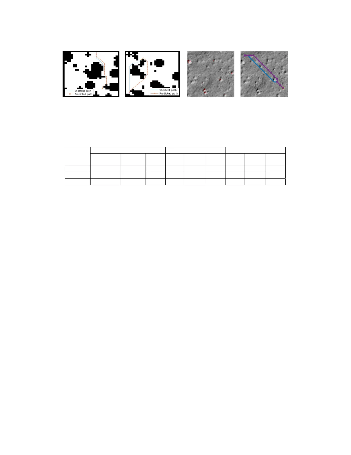
V alue Iteration Networks A viv T amar , Y i W u, Garrett Thomas, Sergey Le vine, and Pieter Abbeel Dept. of Electrical Engineering and Computer Sciences, UC Berkeley Abstract W e introduce the value iteration network (VIN): a fully dif ferentiable neural net- work with a ‘planning module’ embedded within. VINs can learn to plan , and are suitable for predicting outcomes that in volv e planning-based reasoning, such as policies for reinforcement learning. K ey to our approach is a no vel dif ferentiable approximation of the value-iteration algorithm, which can be represented as a con- volutional neural netw ork, and trained end-to-end using standard backpropagation. W e ev aluate VIN based policies on discrete and continuous path-planning domains, and on a natural-language based search task. W e sho w that by learning an explicit planning computation, VIN policies generalize better to new , unseen domains. 1 Introduction Over the last decade, deep conv olutional neural networks (CNNs) have re volutionized supervised learning for tasks such as object recognition, action recognition, and semantic segmentation [ 3 , 15 , 6 , 19 ]. Recently , CNNs have been applied to reinforcement learning (RL) tasks with visual observ ations such as Atari games [ 21 ], robotic manipulation [ 18 ], and imitation learning (IL) [ 9 ]. In these tasks, a neural network (NN) is trained to represent a policy – a mapping from an observation of the system’ s state to an action, with the goal of representing a control strate gy that has good long-term behavior , typically quantified as the minimization of a sequence of time-dependent costs. The sequential nature of decision making in RL is inherently dif ferent than the one-step decisions in supervised learning, and in general requires some form of planning [ 2 ]. Howe ver , most recent deep RL works [ 21 , 18 , 9 ] employed NN architectures that are very similar to the standard networks used in supervised learning tasks, which typically consist of CNNs for feature extraction, and fully connected layers that map the features to a probability distrib ution over actions. Such netw orks are inherently reactive , and in particular, lack explicit planning computation . The success of reactive policies in sequential problems is due to the learning algorithm , which essentially trains a reacti ve policy to select actions that ha ve good long-term consequences in its training domain. T o understand why planning can nevertheless be an important ingredient in a policy , consider the grid-world navig ation task depicted in Figure 1 (left), in which the agent can observe a map of its domain, and is required to navigate between some obstacles to a target position. One hopes that after training a policy to solve se veral instances of this problem with different obstacle configurations, the policy w ould generalize to solve a dif ferent, unseen domain, as in Figure 1 (right). Ho wev er , as we show in our e xperiments, while standard CNN-based networks can be easily trained to solve a set of such maps, they do not generalize well to new tasks outside this set, because they do not understand the goal-directed nature of the beha vior . This observation suggests that the computation learned by reactiv e policies is different from planning, which is required to solv e a new task 1 . 1 In principle, with enough training data that covers all possible task configurations, and a rich enough policy representation, a reacti ve policy can learn to map each task to its optimal polic y . In practice, this is often too expensiv e, and we of fer a more data-efficient approach by exploiting a flexible prior about the planning computation underlying the behavior . 30th Conference on Neural Information Processing Systems (NIPS 2016), Barcelona, Spain. Figure 1: T wo instances of a grid-world domain. T ask is to move to the goal between the obstacles. In this w ork, we propose a NN-based polic y that can ef fectively learn to plan . Our model, termed a value-iteration network (VIN), has a differen- tiable ‘planning program’ embedded within the NN structure. The key to our approach is an observation that the classic value-iteration (VI) planning algo- rithm [ 1 , 2 ] may be represented by a specific type of CNN. By embedding such a VI network module inside a standard feed-forward classifi- cation network, we obtain a NN model that can learn the parameters of a planning computation that yields useful predictions. The VI block is dif ferentiable, and the whole netw ork can be trained using standard backpropagation. This makes our polic y simple to train using standard RL and IL algorithms, and straightforward to integrate with NNs for perception and control. Connections between planning algorithms and recurrent NNs were pre viously explored by Ilin et al. [ 12 ]. Our work builds on related ideas, b ut results in a more broadly applicable policy representation. Our approach is dif ferent from model-based RL [ 25 , 4 ], which requires system identification to map the observ ations to a dynamics model, which is then solv ed for a policy . In many applications, including robotic manipulation and locomotion, accurate system identification is dif ficult, and modelling errors can se verely de grade the policy performance. In such domains, a model-free approach is often preferred [ 18 ]. Since a VIN is just a NN policy , it can be trained model free, without requiring explicit system identification. In addition, the effects of modelling errors in VINs can be mitigated by training the network end-to-end, similarly to the methods in [13, 11]. W e demonstrate the effecti veness of VINs within standard RL and IL algorithms in various problems, among which require visual perception, continuous control, and also natural language based decision making in the W ebNav challenge [ 23 ]. After training, the polic y learns to map an observ ation to a planning computation relev ant for the task, and generate action predictions based on the resulting plan. As we demonstrate, this leads to policies that gener alize better to new , unseen, task instances. 2 Background In this section we provide background on planning, value iteration, CNNs, and policy representations for RL and IL. In the sequel, we shall show that CNNs can implement a particular form of planning computation similar to the value iteration algorithm, which can then be used as a policy for RL or IL. V alue Iteration: A standard model for sequential decision making and planning is the Marko v decision process (MDP) [ 1 , 2 ]. An MDP M consists of states s ∈ S , actions a ∈ A , a re ward function R ( s, a ) , and a transition kernel P ( s 0 | s, a ) that encodes the probability of the next state gi ven the current state and action. A policy π ( a | s ) prescribes an action distribution for each state. The goal in an MDP is to find a polic y that obtains high rew ards in the long term . Formally , the value V π ( s ) of a state under policy π is the expected discounted sum of rew ards when starting from that state and ex ecuting policy π , V π ( s ) . = E π [ P ∞ t =0 γ t r ( s t , a t ) | s 0 = s ] , where γ ∈ (0 , 1) is a discount factor , and E π denotes an expectation over trajectories of states and actions ( s 0 , a 0 , s 1 , a 1 . . . ) , in which actions are selected according to π , and states ev olve according to the transition kernel P ( s 0 | s, a ) . The optimal v alue function V ∗ ( s ) . = max π V π ( s ) is the maximal long-term return possible from a state. A policy π ∗ is said to be optimal if V π ∗ ( s ) = V ∗ ( s ) ∀ s . A popular algorithm for calculating V ∗ and π ∗ is value iteration (VI): V n +1 ( s ) = max a Q n ( s, a ) ∀ s, where Q n ( s, a ) = R ( s, a ) + γ P s 0 P ( s 0 | s, a ) V n ( s 0 ) . (1) It is well known that the value function V n in VI con verges as n → ∞ to V ∗ , from which an optimal policy may be deri ved as π ∗ ( s ) = arg max a Q ∞ ( s, a ) . Con volutional Neural Netw orks (CNNs) are NNs with a particular architecture that has proved useful for computer vision, among other domains [ 8 , 16 , 3 , 15 ]. A CNN is comprised of stacked conv olution and max-pooling layers. The input to each con volution layer is a 3- dimensional signal X , typically , an image with l channels, m horizontal pixels, and n verti- cal pixels, and its output h is a l 0 -channel con volution of the image with kernels W 1 , . . . , W l 0 , h l 0 ,i 0 ,j 0 = σ  P l,i,j W l 0 l,i,j X l,i 0 − i,j 0 − j  , where σ is some scalar activ ation function. A max-pooling layer selects, for each channel l and pixel i, j in h , the maximum value among its neighbors N ( i, j ) , h maxpool l,i,j = max i 0 ,j 0 ∈ N ( i,j ) h l,i 0 ,j 0 . T ypically , the neighbors N ( i, j ) are chosen as a k × k image 2 patch around pixel i, j . After max-pooling, the image is down-sampled by a constant f actor d , com- monly 2 or 4, resulting in an output signal with l 0 channels, m/d horizontal pixels, and n/d vertical pixels. CNNs are typically trained using stochastic gradient descent (SGD), with backpropag ation for computing gradients. Reinfor cement Learning and Imitation Learning: In MDPs where the state space is very large or continuous, or when the MDP transitions or re wards are not known in adv ance, planning algorithms cannot be applied. In these cases, a policy can be learned from either expert supervision – IL, or by trial and error – RL. While the learning algorithms in both cases are different, the policy representations – which are the focus of this w ork – are similar . Additionally , most state-of-the-art algorithms such as [ 24 , 21 , 26 , 18 ] are agnostic to the policy representation, and only require it to be differentiable, for performing gradient descent on some algorithm-specific loss function. Therefore, in this paper we do not commit to a specific learning algorithm, and only consider the policy . Let φ ( s ) denote an observation for state s . The policy is specified as a parametrized function π θ ( a | φ ( s )) mapping observations to a probability ov er actions, where θ are the policy parameters. For example, the policy could be represented as a neural network, with θ denoting the network weights. The goal is to tune the parameters such that the policy behav es well in the sense that π θ ( a | φ ( s )) ≈ π ∗ ( a | φ ( s )) , where π ∗ is the optimal policy for the MDP , as defined in Section 2. In IL, a dataset of N state observations and corresponding optimal actions  φ ( s i ) , a i ∼ π ∗ ( φ ( s i ))  i =1 ,...,N is generated by an expert. Learning a policy then becomes an instance of supervised learning [ 24 , 9 ]. In RL, the optimal action is not av ailable, but instead, the agent can act in the w orld and observe the rewards and state transitions its actions effect. RL algorithms such as in [27, 21, 26, 18] use these observations to impro ve the v alue of the policy . 3 The V alue Iteration Network Model In this section we introduce a general policy representation that embeds an explicit planning module . As stated earlier , the moti vation for such a representation is that a natural solution to man y tasks, such as the path planning described abov e, in volves planning on some model of the domain. Let M denote the MDP of the domain for which we design our policy π . W e assume that there is some unknown MDP ¯ M such that the optimal plan in ¯ M contains useful information about the optimal policy in the original task M . Howe ver , we emphasize that we do not assume to know ¯ M in adv ance. Our idea is to equip the policy with the ability to learn and solve ¯ M , and to add the solution of ¯ M as an element in the policy π . W e hypothesize that this will lead to a policy that automatically learns a useful ¯ M to plan on. W e denote by ¯ s ∈ ¯ S , ¯ a ∈ ¯ A , ¯ R ( ¯ s, ¯ a ) , and ¯ P ( ¯ s 0 | ¯ s, ¯ a ) the states, actions, rew ards, and transitions in ¯ M . T o facilitate a connection between M and ¯ M , we let ¯ R and ¯ P depend on the observation in M , namely , ¯ R = f R ( φ ( s )) and ¯ P = f P ( φ ( s )) , and we will later learn the functions f R and f P as a part of the policy learning process. For example, in the grid-world domain described abov e, we can let ¯ M hav e the same state and action spaces as the true grid-world M . The reward function f R can map an image of the domain to a high reward at the goal, and negati ve rew ard near an obstacle, while f P can encode deterministic mov ements in the grid-world that do not depend on the observation. While these rew ards and transitions are not necessarily the true rewards and transitions in the task, an optimal plan in ¯ M will still follow a trajectory that a voids obstacles and reaches the goal, similarly to the optimal plan in M . Once an MDP ¯ M has been specified, any standard planning algorithm can be used to obtain the v alue function ¯ V ∗ . In the next section, we shall sho w that using a particular implementation of VI for planning has the advantage of being differentiable, and simple to implement within a NN framework. In this section howe ver , we focus on how to use the planning result ¯ V ∗ within the NN policy π . Our approach is based on two important observations. The first is that the v ector of values ¯ V ∗ ( s ) ∀ s encodes all the information about the optimal plan in ¯ M . Thus, adding the v ector ¯ V ∗ as additional features to the policy π is sufficient for e xtracting information about the optimal plan in ¯ M . Howe ver , an additional property of ¯ V ∗ is that the optimal decision ¯ π ∗ ( ¯ s ) at a state ¯ s can depend only on a subset of the v alues of ¯ V ∗ , since ¯ π ∗ ( ¯ s ) = arg max ¯ a ¯ R ( ¯ s, ¯ a ) + γ P ¯ s 0 ¯ P ( ¯ s 0 | ¯ s, ¯ a ) ¯ V ∗ ( ¯ s 0 ) . Therefore, if the MDP has a local connectivity structure, such as in the grid-world e xample abov e, the states for which ¯ P ( ¯ s 0 | ¯ s, ¯ a ) > 0 is a small subset of ¯ S . In NN terminology , this is a form of attention [ 32 ], in the sense that for a given label prediction (action), only a subset of the input features (value function) is relev ant. Attention is known to improve learning performance by reducing the ef fectiv e number of network parameters during learning. Therefore, the second element in our network is an attention module that outputs a v ector of (attention 3 modulated) v alues ψ ( s ) . Finally , the vector ψ ( s ) is added as additional features to a reacti ve policy π re ( a | φ ( s ) , ψ ( s )) . The full network architecture is depicted in Figure 2 (left). Returning to our grid-world e xample, at a particular state s , the reacti ve policy only needs to query the values of the states neighboring s in order to select the correct action. Thus, the attention module in this case could return a ψ ( s ) vector with a subset of ¯ V ∗ for these neighboring states. K recurrence Reward Q Prev. Value New Value VI Module P R V Figure 2: Planning-based NN models. Left: a general policy representation that adds v alue function features from a planner to a reactiv e policy . Right: VI module – a CNN representation of VI algorithm. Let θ denote all the parameters of the policy , namely , the parameters of f R , f P , and π re , and note that ψ ( s ) is in fact a function of φ ( s ) . Therefore, the polic y can be written in the form π θ ( a | φ ( s )) , similarly to the standard policy form (cf. Section 2). If we could back-propagate through this function, then potentially we could train the policy using standard RL and IL algorithms, just like any other standard policy representation. While it is easy to design functions f R and f P that are differentiable (and we provide sev eral examples in our experiments), back-propagating the gradient through the planning algorithm is not tri vial. In the following, we propose a no vel interpretation of an approximate VI algorithm as a particular form of a CNN. This allows us to con veniently treat the planning module as just another NN, and by back-propagating through it, we can train the whole policy end-to-end . 3.1 The VI Module W e now introduce the VI module – a NN that encodes a differentiable planning computation. Our starting point is the VI algorithm (1) . Our main observation is that each iteration of VI may be seen as passing the previous value function V n and rew ard function R through a con volution layer and max-pooling layer . In this analogy , each channel in the con v olution layer corresponds to the Q -function for a specific action, and conv olution kernel weights correspond to the discounted transition probabilities. Thus by recurrently applying a con volution layer K times, K iterations of VI are effecti vely performed. Follo wing this idea, we propose the VI network module, as depicted in Figure 2B. The inputs to the VI module is a ‘rew ard image’ ¯ R of dimensions l, m, n , where here, for the purpose of clarity , we follow the CNN formulation and explicitly assume that the state space ¯ S maps to a 2-dimensional grid. Ho wev er, our approach can be extended to general discrete state spaces, for example, a graph, as we report in the W ikiNav e xperiment in Section 4.4. The re ward is fed into a con volutional layer ¯ Q with ¯ A channels and a linear acti vation function, ¯ Q ¯ a,i 0 ,j 0 = P l,i,j W ¯ a l,i,j ¯ R l,i 0 − i,j 0 − j . Each channel in this layer corresponds to ¯ Q ( ¯ s, ¯ a ) for a particular action ¯ a . This layer is then max-pooled along the actions channel to produce the next-iteration value function layer ¯ V , ¯ V i,j = max ¯ a ¯ Q (¯ a, i, j ) . The next-iteration v alue function layer ¯ V is then stacked with the reward ¯ R , and fed back into the con volutional layer and max-pooling layer K times, to perform K iterations of value iteration. The VI module is simply a NN architecture that has the capability of performing an approximate VI computation. Nev ertheless, representing VI in this form mak es learning the MDP parameters and rew ard function natural – by backpropagating through the network, similarly to a standard CNN. VI modules can also be composed hierarchically , by treating the value of one VI module as additional input to another VI module. W e further report on this idea in the supplementary material. 3.2 V alue Iteration Networks W e no w hav e all the ingredients for a dif ferentiable planning-based policy , which we term a v alue iteration network (VIN). The VIN is based on the general planning-based policy defined abov e, with the VI module as the planning algorithm. In order to implement a VIN, one has to specify the state 4 and action spaces for the planning module ¯ S and ¯ A , the re ward and transition functions f R and f P , and the attention function; we refer to this as the VIN design . F or some tasks, as we sho w in our experiments, it is relati vely straightforward to select a suitable design, while other tasks may require more thought. Howe ver , we emphasize an important point: the reward, transitions, and attention can be defined by parametric functions, and trained with the whole policy 2 . Thus, a rough design can be specified, and then fine-tuned by end-to-end training. Once a VIN design is chosen, implementing the VIN is straightforward, as it is simply a form of a CNN. The networks in our experiments all required only se veral lines of Theano [ 28 ] code. In the next section, we e v aluate VIN policies on various domains, showing that by learning to plan, the y achiev e a better generalization capability . 4 Experiments In this section we ev aluate VINs as policy representations on various domains. Additional experiments in vestigating RL and hierarchical VINs, as well as technical implementation details are discussed in the supplementary material. Source code is av ailable at https://github.com/avivt/VIN . Our goal in these experiments is to in vestigate the follo wing questions: 1. Can VINs effecti vely learn a planning computation using standard RL and IL algorithms? 2. Does the planning computation learned by VINs make them better than reacti ve policies at generalizing to new domains? An additional goal is to point out several ideas for designing VINs for various tasks. While this is not an exhausti ve list that fits all domains, we hope that it will moti vate creati ve designs in future work. 4.1 Grid-W orld Domain Our first experiment domain is a synthetic grid-world with randomly placed obstacles, in which the observation includes the position of the agent, and also an image of the map of obstacles and goal position. Figure 3 shows tw o random instances of such a grid-world of size 16 × 16 . W e conjecture that by learning the optimal policy for several instances of this domain, a VIN policy would learn the planning computation required to solve a ne w , unseen, task. In such a simple domain, an optimal policy can easily be calculated using exact VI. Note, ho wev er , that here we are interested in evaluating whether a NN polic y , trained using RL or IL, can learn to plan . In the following results, policies were trained using IL, by standard supervised learning from demonstrations of the optimal polic y . In the supplementary material, we report additional RL experiments that sho w similar findings. W e design a VIN for this task following the guidelines described above, where the planning MDP ¯ M is a grid-w orld, similar to the true MDP . The reward mapping f R is a CNN mapping the image input to a rew ard map in the grid-world. Thus, f R should potentially learn to discriminate between obstacles, non-obstacles and the goal, and assign a suitable re ward to each. The transitions ¯ P were defined as 3 × 3 con volution k ernels in the VI block, exploiting the fact that transitions in the grid-world are local 3 . The recurrence K was chosen in proportion to the grid-world size, to ensure that information can flow from the goal state to any other state. F or the attention module, we chose a trivial approach that selects the ¯ Q values in the VI block for the current state, i.e., ψ ( s ) = ¯ Q ( s, · ) . The final reactiv e policy is a fully connected network that maps ψ ( s ) to a probability ov er actions. W e compare VINs to the following NN reactiv e policies: CNN network: W e devised a CNN-based reactiv e policy inspired by the recent impressiv e results of DQN [ 21 ], with 5 con v olution layers, and a fully connected output. While the network in [ 21 ] was trained to predict Q v alues, our network outputs a probability ov er actions. These terms are related, since π ∗ ( s ) = arg max a Q ( s, a ) . Fully Conv olutional Netw ork (FCN): The problem setting for this domain is similar to semantic segmentation [19], in which each pix el in the image is assigned a semantic label (the action in our case). W e therefore de vised an FCN inspired by a state-of-the-art semantic segmentation algorithm [ 19 ], with 3 conv olution layers, where the first layer has a filter that spans the whole image, to properly con ve y information from the goal to ev ery other state. In T able 1 we present the average 0 − 1 prediction loss of each model, ev aluated on a held-out test-set of maps with random obstacles, goals, and initial states, for different problem sizes. In addition, for each map, a full trajectory from the initial state w as predicted, by iterati vely rolling-out the ne xt-states 2 VINs are fundamentally dif ferent than in verse RL methods [ 22 ], where transitions are required to be known. 3 Note that the transitions defined this w ay do not depend on the state ¯ s . Interestingly , we shall see that the network learned to plan successful trajectories ne vertheless, by appropriately shaping the re ward. 5 Figure 3: Grid-world domains (best viewed in color). A,B: T wo random instances of the 28 × 28 synthetic gridworld, with the VIN-predicted trajectories and ground-truth shortest paths between random start and goal positions. C: An image of the Mars domain, with points of elev ation sharper than 10 ◦ colored in red. These points were calculated from a matching image of elev ation data (not sho wn), and were not a vailable to the learning algorithm. Note the difficulty of distinguishing between obstacles and non-obstacles. D: The VIN-predicted (purple line with cross markers), and the shortest-path ground truth (blue line) trajectories between between random start and goal positions. Domain VIN CNN FCN Prediction Success T raj. Pred. Succ. T raj. Pred. Succ. T raj. loss rate diff. loss rate diff. loss rate dif f. 8 × 8 0.004 99.6% 0.001 0.02 97.9% 0.006 0.01 97.3% 0.004 16 × 16 0.05 99.3% 0.089 0.10 87.6% 0.06 0.07 88.3% 0.05 28 × 28 0.11 97% 0.086 0.13 74.2% 0.078 0.09 76.6% 0.08 T able 1: Performance on grid-world domain. T op: comparison with reactive policies. For all domain sizes, VIN networks significantly outperform standard reacti ve networks. Note that the performance gap increases dramatically with problem size. predicted by the network. A trajectory was said to succeed if it reached the goal without hitting obstacles. For each trajectory that succeeded, we also measured its difference in length from the optimal trajectory . The av erage difference and the a verage success rate are reported in T able 1. Clearly , VIN policies generalize to domains outside the training set. A visualization of the re ward mapping f R (see supplementary material) sho ws that it is negati ve at obstacles, positi ve at the goal, and a small negati ve constant otherwise. The resulting value function has a gradient pointing towards a direction to the goal around obstacles, thus a useful planning computation was learned. VINs also significantly outperform the reactiv e networks, and the performance gap increases dramatically with the problem size. Importantly , note that the prediction loss for the reactiv e policies is comparable to the VINs, although their success rate is significantly worse. This shows that this is not a standard case of ov erfitting/underfitting of the reacti ve policies. Rather , VIN policies, by their VI structure, focus prediction errors on less important parts of the trajectory , while reactiv e policies do not make this distinction, and learn the easily predictable parts of the trajectory yet fail on the complete task. The VINs hav e an eff ective depth of K , which is larger than the depth of the reactive policies. One may wonder , whether any deep enough network w ould learn to plan. In principle, a CNN or FCN of depth K has the potential to perform the same computation as a VIN. Ho wev er , it has much more parameters, requiring much more training data. W e ev aluate this by untying the weights in the K recurrent layers in the VIN. Our results, reported in the supplementary material, show that untying the weights degrades performance, with a stronger ef fect for smaller sizes of training data. 4.2 Mars Rover Navigation In this experiment we show that VINs can learn to plan from natural image input . W e demonstrate this on path-planning from ov erhead terrain images of a Mars landscape. Each domain is represented by a 128 × 128 image patch, on which we defined a 16 × 16 grid-world, where each state was considered an obstacle if the terrain in its corresponding 8 × 8 image patch contained an ele vation angle of 10 degrees or more, e v aluated using an external ele vation data base. An example of the domain and terrain image is depicted in Figure 3. The MDP for shortest-path planning in this case is similar to the grid-world domain of Section 4.1, and the VIN design was similar , only with a deeper CNN in the rew ard mapping f R for processing the image. The policy was trained to predict the shortest-path dir ectly fr om the terrain image . W e emphasize that the elev ation data is not part of the input , and must be inferred (if needed) from the terrain image. 6 After training, VIN achie ved a success rate of 84 . 8 %. T o put this rate in context, we compare with the best performance achiev able without access to the elev ation data, which is 90 . 3 %. T o make this comparison, we trained a CNN to classify whether an 8 × 8 patch is an obstacle or not. This classifier w as trained using the same image data as the VIN network, but its labels were the true obstacle classifications from the elev ation map (we reiterate that the VIN did not have access to these ground-truth obstacle labels during training or testing). The success rate of planner that uses the obstacle map generated by this classifier from the raw image is 90 . 3 %, showing that obstacle identification from the raw image is indeed challenging. Thus, the success rate of the VIN, which was trained without any obstacle labels, and had to ‘figure out’ the planning process is quite remarkable. 4.3 Continuous Control Network Train Error T est Error VIN 0.30 0.35 CNN 0.39 0.59 Figure 4: Continuous control domain. T op: av er- age distance to goal on training and test domains for VIN and CNN policies. Bottom: trajectories predicted by VIN and CNN on test domains. W e now consider a 2D path planning domain with continuous states and continuous actions , which cannot be solved using VI, and therefore a VIN cannot be naiv ely applied. Instead, we will construct the VIN to perform ‘high-le vel’ planning on a discrete, coarse, grid-world rep- resentation of the continuous domain. W e shall show that a VIN can learn to plan such a ‘high- lev el’ plan, and also exploit that plan within its ‘low-le vel’ continuous control policy . Moreo ver , the VIN policy results in better generalization than a reactiv e policy . Consider the domain in Figure 4. A red-colored particle needs to be navigated to a green goal us- ing horizontal and vertical forces. Gray-colored obstacles are randomly positioned in the domain, and apply an elastic force and friction when contacted. This domain presents a non-trivial control problem, as the agent needs to both plan a feasible trajectory between the obstacles (or use them to bounce of f), but also control the particle (which has mass and inertia) to follo w it. The state obser - vation consists of the particle’ s continuous position and velocity , and a static 16 × 16 downscaled image of the obstacles and goal position in the domain. In principle, such an observation is suf ficient to devise a ‘rough plan’ for the particle to follo w . As in our pre vious experiments, we in vestigate whether a policy trained on se veral instances of this domain with different start state, goal, and obstacle positions, would generalize to an unseen domain. For training we chose the guided policy search (GPS) algorithm with unknown dynamics [ 17 ], which is suitable for learning policies for continuous dynamics with contacts, and we used the publicly av ailable GPS code [ 7 ], and Mujoco [ 30 ] for physical simulation. W e generated 200 random training instances, and ev aluate our performance on 40 differ ent test instances from the same distribution. Our VIN design is similar to the grid-world cases, with some important modifications: the attention module selects a 5 × 5 patch of the value ¯ V , centered around the current (discretized) position in the map. The final reactive polic y is a 3-layer fully connected network, with a 2-dimensional continuous output for the controls. In addition, due to the limited number of training domains, we pre-trained the VIN with transition weights that correspond to discounted grid-world transitions. This is a reasonable prior for the weights in a 2-d task, and we emphasize that e ven with this initialization, the initial value function is meaningless, since the rew ard map f R is not yet learned. W e compare with a CNN-based reactiv e policy inspired by the state-of-the-art results in [ 21 , 20 ], with 2 CNN layers for image processing, followed by a 3-layer fully connected netw ork similar to the VIN reactiv e policy . Figure 4 sho ws the performance of the trained policies, measured as the final distance to the target. The VIN clearly outperforms the CNN on test domains. W e also plot se veral trajectories of both policies on test domains, showing that VIN learned a more sensible generalization of the task. 4.4 W ebNav Challenge In the previous e xperiments, the planning aspect of the task corresponded to 2D navigation. W e now consider a more general domain: W ebNav [23] – a language based search task on a graph. In W ebNav [ 23 ], the agent needs to na vigate the links of a website to wards a goal web-page, specified by a short 4-sentence query . At each state s (web-page), the agent can observe av erage word- embedding features of the state φ ( s ) and possible next states φ ( s 0 ) (linked pages), and the features of the query φ ( q ) , and based on that has to select which link to follow . In [ 23 ], the search was performed 7 on the W ikipedia website. Here, we report experiments on the ‘W ikipedia for Schools’ website, a simplified W ikipedia designed for children, with ov er 6000 pages and at most 292 links per page. In [ 23 ], a NN-based policy was proposed, which first learns a NN mapping from ( φ ( s ) , φ ( q )) to a hidden state vector h . The action is then selected according to π ( s 0 | φ ( s ) , φ ( q )) ∝ exp  h > φ ( s 0 )  . In essence, this policy is reactiv e, and relies on the word embedding features at each state to contain meaningful information about the path to the goal. Indeed, this property naturally holds for an encyclopedic website that is structured as a tree of categories, sub-categories, sub-sub-cate gories, etc. W e sought to explore whether planning, based on a VIN, can lead to better performance in this task, with the intuition that a plan on a simplified model of the website can help guide the reactiv e policy in dif ficult queries. Therefore, we designed a VIN that plans on a small subset of the graph that contains only the 1st and 2nd lev el categories ( < 3 % of the graph), and their word-embedding features. Designing this VIN requires a different approach from the grid-world VINs described earlier , where the most challenging aspect is to define a meaningful mapping between nodes in the true graph and nodes in the smaller VIN graph. F or the re ward mapping f R , we chose a weighted similarity measure between the query features φ ( q ) , and the features of nodes in the small graph φ ( ¯ s ) . Thus, intuitiv ely , nodes that are similar to the query should hav e high reward. The transitions were fixed based on the graph connecti vity of the smaller VIN graph, which is kno wn, though different from the true graph. The attention module was also based on a weighted similarity measure between the features of the possible next states φ ( s 0 ) and the features of each node in the simplified graph φ ( ¯ s ) . The reacti ve policy part of the VIN was similar to the policy of [ 23 ] described above. Note that by training such a VIN end-to-end, we are effecti vely learning ho w to exploit the small graph for doing better planning on the true, large graph. Both the VIN policy and the baseline reactiv e policy were trained by supervised learning, on random trajectories that start from the root node of the graph. Similarly to [ 23 ], a policy is said to succeed a query if all the correct predictions along the path are within its top-4 predictions. After training, the VIN policy performed mildly better than the baseline on 2000 held-out test queries when starting from the root node, achieving 1030 successful runs vs. 1025 for the baseline. Ho we ver , when we tested the policies on a harder task of starting from a random position in the graph, VINs significantly outperformed the baseline, achie ving 346 successful runs vs. 304 for the baseline, out of 4000 test queries. These results confirm that indeed, when navigating a tree of cate gories from the root up, the features at each state contain meaningful information about the path to the goal, making a reacti ve policy suf ficient. Ho wev er , when starting the navigation from a different state, a reacti ve policy may fail to understand that it needs to first go back to the root and switch to a different branch in the tree. Our results indicate such a strategy can be better represented by a VIN. W e remark that there is still room for further improvements of the W ebNav results, e.g., by better models for rew ard and attention functions, and better word-embedding representations of text. 5 Conclusion and Outlook The introduction of powerful and scalable RL methods has opened up a range of ne w problems for deep learning. Howev er , few recent works in vestigate policy architectures that are specifically tailored for planning under uncertainty , and current RL theory and benchmarks rarely in vestigate the generalization properties of a trained polic y [ 27 , 21 , 5 ]. This work tak es a step in this direction, by exploring better generalizing polic y representations. Our VIN policies learn an approximate planning computation rele vant for solving the task, and we hav e shown that such a computation leads to better generalization in a div erse set of tasks, ranging from simple gridworlds that are amenable to v alue iteration, to continuous control, and e ven to navigation of W ikipedia links. In future work we intend to learn different planning computations, based on simulation [ 10 ], or optimal linear control [ 31 ], and combine them with reactiv e policies, to potentially dev elop RL solutions for task and motion planning [14]. Acknowledgments This research was funded in part by Siemens, by ONR through a PECASE a ward, by the Army Research Office through the MAST program, and by an NSF CAREER a ward (#1351028). A. T . was partially funded by the V iterbi Scholarship, T echnion. Y . W . was partially funded by a D ARP A PP AML program, contract F A8750-14-C-0011. 8 References [1] R. Bellman. Dynamic Pr ogramming . Princeton Uni versity Press, 1957. [2] D. Bertsekas. Dynamic Pr ogramming and Optimal Control, V ol II . Athena Scientific, 4th edition, 2012. [3] D. Ciresan, U. Meier, and J. Schmidhuber . Multi-column deep neural networks for image classification. In Computer V ision and P attern Recognition , pages 3642–3649, 2012. [4] M. Deisenroth and C. E. Rasmussen. Pilco: A model-based and data-efficient approach to policy search. In ICML , 2011. [5] Y . Duan, X. Chen, R. Houthooft, J. Schulman, and P . Abbeel. Benchmarking deep reinforcement learning for continuous control. arXiv pr eprint arXiv:1604.06778 , 2016. [6] C. Farabet, C. Couprie, L. Najman, and Y . LeCun. Learning hierarchical features for scene labeling. IEEE T ransactions on P attern Analysis and Machine Intelligence , 35(8):1915–1929, 2013. [7] C. Finn, M. Zhang, J. Fu, X. T an, Z. McCarthy , E. Scharff, and S. Levine. Guided policy search code implementation, 2016. Software av ailable from rll.berkeley .edu/gps. [8] K. Fukushima. Neural network model for a mechanism of pattern recognition unaffected by shift in position- neocognitron. T ransactions of the IECE , J62-A(10):658–665, 1979. [9] A. Giusti et al. A machine learning approach to visual perception of forest trails for mobile robots. IEEE Robotics and Automation Letters , 2016. [10] X. Guo, S. Singh, H. Lee, R. L. Lewis, and X. W ang. Deep learning for real-time atari game play using offline monte-carlo tree search planning. In NIPS , 2014. [11] X. Guo, S. Singh, R. Lewis, and H. Lee. Deep learning for rew ard design to improve monte carlo tree search in atari games. , 2016. [12] R. Ilin, R. K ozma, and P . J. W erbos. Efficient learning in cellular simultaneous recurrent neural netw orks-the case of maze navigation problem. In ADPRL , 2007. [13] J. Joseph, A. Geramifard, J. W . Roberts, J. P . How , and N. Roy . Reinforcement learning with misspecified model classes. In ICRA , 2013. [14] L. P . Kaelbling and T . Lozano-Pérez. Hierarchical task and motion planning in the no w . In IEEE International Conference on Robotics and Automation (ICRA) , pages 1470–1477, 2011. [15] A. Krizhevsky , I. Sutsk ever , and G. Hinton. Imagenet classification with deep conv olutional neural networks. In NIPS , 2012. [16] Y . LeCun, L. Bottou, Y . Bengio, and P . Haf fner . Gradient-based learning applied to document recognition. Pr oceedings of the IEEE , 86(11):2278–2324, 1998. [17] S. Levine and P . Abbeel. Learning neural network policies with guided policy search under unknown dynamics. In NIPS , 2014. [18] S. Levine, C. Finn, T . Darrell, and P . Abbeel. End-to-end training of deep visuomotor policies. JMLR , 17, 2016. [19] J. Long, E. Shelhamer , and T . Darrell. Fully conv olutional networks for semantic segmentation. In IEEE Confer ence on Computer V ision and P attern Recognition , pages 3431–3440, 2015. [20] V . Mnih, A. P . Badia, M. Mirza, A. Graves, T . Lillicrap, T . Harley , D. Silver , and K. Kavukcuoglu. Asynchronous methods for deep reinforcement learning. arXiv pr eprint arXiv:1602.01783 , 2016. [21] V . Mnih, K. Ka vukcuoglu, D. Silver , A. Rusu, J. V eness, M. Bellemare, A. Graves, M. Riedmiller , A. Fidjeland, G. Ostro vski, et al. Human-lev el control through deep reinforcement learning. Nature , 518(7540):529–533, 2015. [22] G. Neu and C. Szepesvári. Apprenticeship learning using in verse reinforcement learning and gradient methods. In UAI , 2007. [23] R. Nogueira and K. Cho. W ebnav: A new lar ge-scale task for natural language based sequential decision making. arXiv pr eprint arXiv:1602.02261 , 2016. [24] S. Ross, G. Gordon, and A. Bagnell. A reduction of imitation learning and structured prediction to no-regret online learning. In AIST ATS , 2011. [25] J. Schmidhuber . An on-line algorithm for dynamic reinforcement learning and planning in reactive en vironments. In International Joint Conference on Neural Networks . IEEE, 1990. [26] J. Schulman, S. Le vine, P . Abbeel, M. Jordan, and P . Moritz. T rust region polic y optimization. In ICML , 2015. [27] R. S. Sutton and A. G. Barto. Reinfor cement learning: An intr oduction . MIT press, 1998. [28] Theano Dev elopment T eam. Theano: A Python frame work for fast computation of mathematical expres- sions. arXiv e-prints , abs/1605.02688, May 2016. [29] T . Tieleman and G. Hinton. Lecture 6.5. COURSERA: Neural Networks for Machine Learning, 2012. [30] E. T odorov , T . Erez, and Y . T assa. Mujoco: A ph ysics engine for model-based control. In Intelligent Robots and Systems (IR OS), 2012 IEEE/RSJ International Conference on , pages 5026–5033. IEEE, 2012. [31] M. W atter , J. Springenberg, J. Boedecker, and M. Riedmiller . Embed to control: A locally linear latent dynamics model for control from raw images. In NIPS , 2015. [32] K. Xu, J. Ba, R. Kiros, K. Cho, A. Courville, R. Salakhudinov , R. Zemel, and Y . Bengio. Sho w , attend and tell: Neural image caption generation with visual attention. In ICML , 2015. 9 A V isualization of Learned Reward and V alue In Figure 5 we plot the learned reward and v alue function for the gridworld task. The learned reward is very ne gati ve at obstacles, v ery positiv e at goal, and a slightly ne gativ e constant otherwise. The resulting value function has a peak at the goal, and a gradient pointing towards a direction to the goal around obstacles. This plot clearly shows that the VI block learned a useful planning computation. Figure 5: V isualization of learned reward and v alue function. Left: a sample domain. Center: learned rew ard f R for this domain. Right: resulting value function (in VI block) for this domain. B W eight Sharing The VINs hav e an eff ective depth of K , which is larger than the depth of the reactive policies. One may wonder , whether any deep enough netw ork would learn to plan. In principle, a CNN or FCN of depth K has the potential to perform the same computation as a VIN. Howe ver , it has much more parameters, requiring much more training data. W e e valuate this by untying the weights in the K recurrent layers in the VIN. Our results, in T able 2 show that untying the weights degrades performance, with a stronger effect for smaller sizes of training data. T raining data VIN VIN Untied W eights Pred. Succ. T raj. Pred. Succ. T raj. loss rate diff. loss rate dif f. 20% 0.06 98.2% 0.106 0.09 91.9% 0.094 50% 0.05 99.4% 0.018 0.07 95.2% 0.078 100% 0.05 99.3% 0.089 0.05 95.6% 0.068 T able 2: Performance on 16 × 16 grid-world domain. Ev aluation of the ef fect of VI module shared weights relativ e to data size. C Gridw orld with Reinf orcement Learning W e demonstrate that the value iteration network can be trained using reinforcement learning methods and achie ves fa vorable generalization properties as compared to standard con volutional neural networks (CNNs). The overall setup of the experiment is as follows: we train policies parameterized by VINs and policies parameterized by con volutional netw orks on the same set of randomly generated gridworld maps in the same way (described belo w) and then test their performance on a held-out set of test maps, which was generated in the same way as the set of training maps but is disjoint from the training set. The MDP is what one would expect of a gridw orld en vironment – the states are the positions on the map; the actions are mo vements up, do wn, left, and right; the re wards are +1 for reaching the goal, − 1 for falling into a hole, and − 0 . 01 otherwise (to encourage the polic y to find the shortest path); the transitions are deterministic. Structure of the networks. The VINs used are similar to those described in the main body of the paper . After K value-iteration recurrences, we hav e approximate Q values for e very state and action in the map. The attention selects only those for the current state, and these are con verted to a 10 Network 8 × 8 16 × 16 VIN 90.9% 82.5% CNN 86.9% 33.1% T able 3: RL Results – performance on test maps. probability distribution o ver actions using the softmax function. W e use K = 10 for the 8 × 8 maps and K = 20 for the 16 × 16 maps. The con volutional networks’ structure was adapted to accommodate the size of the maps. For the 8 × 8 maps, we use 50 filters in the first layer and then 100 filters in the second layer , all of size 3 × 3 . Each of these layers is follo wed by a 2 × 2 max-pool. At the end we ha ve a fully connected hidden layer with 100 hidden units, followed by a fully-connected layer to the (4) outputs, which are conv erted to probabilities using the softmax function. The network for the 16 × 16 maps is similar b ut uses three con volutional layers (with 50, 100, and 100 filters respectively), the first tw o of which are 2 × 2 max-pooled, follo wed by two fully-connected hidden layers (200 and 100 hidden units respectively) before connecting to the outputs and performing softmax. T raining with a curriculum. T o ensure that the policies are not simply memorizing specific maps, we randomly select a map before each episode. But some maps are far more difficult than others, and the agent learns best when it stands a reasonable chance of reaching this goal. Thus we found it beneficial to begin training on the easiest maps and then gradually progress to more difficult maps. This is the idea of curriculum training . W e consider curriculum training as a way to address the exploration problem. If a completely untrained agent is dropped into a very challenging map, it moves randomly and stands approximately zero chance of reaching the goal (and thus learning a useful re ward). But e ven a random policy can consistently reach goals nearby and learn something useful in the process, e.g. to mov e to ward the goal. Once the policy knows how to solve tasks of difficulty n , it can more easily learn to solve tasks of difficulty n + 1 , as compared to a completely untrained policy . This strategy is well-aligned with how formal education is structured; you can’ t effecti vely learn calculus without kno wing basic algebra. Not all en vironments hav e an obvious dif ficulty metric, but fortunately the gridworld task does. W e define the dif ficulty of a map as the length of the shortest path from the start state to the goal state. It is natural to start with difficulty 1 (the start state and goal state are adjacent) and ramp up the dif ficulty by one lev el once a certain threshold of “success” is reached. In our experiments we use the av erage discounted return to assess progress and increase the dif ficulty le vel from n to n + 1 when the av erage discounted return for an iteration exceeds 1 − n 35 . This rule was chosen empirically and takes into account the fact that higher dif ficulty le vels are more dif ficult to learn. All networks were trained using the trust region polic y optimization (TRPO) [ 26 ] algorithm, using publicly av ailable code in the RLLab benchmark [5]. T esting. When testing, we ignore the exact rewards and measure simply whether or not the agent reaches the goal. For each map in the test set, we run an episode, noting if the policy succeeds in reaching the goal. The proportion of successful trials out of all the trials is reported for each network. (See T able 3.) On the 8 × 8 maps, we used the same number of training iterations on both types of networks to make the comparison as fair as possible. On the 16 × 16 maps, it became clear that the conv olutional network was struggling, so we allo wed it twice as many training iterations as the VIN, yet it still failed to achie ve e ven a remotely similar level of performance on the test maps. (See left image of Figure 6.) W e posit that this is because the VIN learns to plan, while the CNN simply follows a reactiv e policy . Though the CNN policy performs reasonably well on the smaller domains, it does not scale to larger domains, while the VIN does. (See right image of Figure 6.) D T echnical Details for Experiments W e report the full technical details used for training our networks. 11 Figure 6: RL results – performance of VIN and CNN on 16 × 16 test maps. Left: Performance on all maps as a function of amount of training. Right: Success rate on test maps of increasing difficulty . D.1 Grid-world Domain Our training set consists of N i = 5000 random grid-world instances, with N t = 7 shortest-path trajectories (calculated using an optimal planning algorithm) from a random start-state to a random goal-state for each instance; a total of N i × N t trajectories. For each state s = ( i, j ) in each trajectory , we produce a (2 × m × n ) -sized observation image s image . The first channel of s image encodes the obstacle presence (1 for obstacle, 0 otherwise), while the second channel encodes the goal position (1 at the goal, 0 otherwise). The full observation v ector is φ ( s ) = [ s, s image ] . In addition, for each state we produce a label a that encodes the action (one of 8 directions) that an optimal shortest-path policy would take in that state. W e design a VIN for this task as follo ws. The state space ¯ S was chosen to be a m × n grid-world, similar to the true state space S . 4 The reward ¯ R in this space can be represented by an m × n map, and we chose the re ward mapping f R to be a CNN with s image as its input, one layer with 150 kernels of size 3 × 3 , and a second layer with one 3 × 3 filter to output ¯ R . Thus, f R maps the image of obstacles and goal to a ‘re ward image’. The transitions ¯ P were defined as 3 × 3 con volution kernels in the VI block, and exploit the f act that transitions in the grid-world are local. Note that the transitions defined this way do not depend on the state ¯ s . Interestingly , we shall see that the network learned re wards and transitions that ne vertheless enable it to successfully plan in this task. For the attention module, since there is a one-to-one mapping between the agent position in S and in ¯ S , we chose a trivial approach that selects the ¯ Q values in the VI block for the state in the real MDP s , i.e., ψ ( s ) = ¯ Q ( s, · ) . The final reactiv e policy is a fully connected softmax output layer with weights W , π re ( ·| ψ ( s )) ∝ exp  W > ψ ( s )  . W e trained se veral neural-netw ork policies based on a multi-class logistic regression loss function using stochastic gradient descent, with an RMSProp step size [ 29 ], implemented in the Theano [ 28 ] library . W e compare the policies: VIN network W e used the VIN model of Section 3 as described above, with 10 channels for the q layer in the VI block. The recurrence K was set relative to the problem size: K = 10 for 8 × 8 domains, K = 20 for 16 × 16 domains, and K = 36 for 28 × 28 domains. The guideline for choosing these values was to keep the network small while guaranteeing that goal information can flow to ev ery state in the map. CNN network: W e de vised a CNN-based reacti ve policy inspired by the recent impressiv e results of DQN [ 21 ], with 5 con volution layers with [50 , 50 , 100 , 100 , 100] kernels of size 3 × 3 , and 2 × 2 max-pooling after the first and third layers. The final layer is fully connected, and maps to a softmax ov er actions. T o represent the current state, we added to s image a channel that encodes the current position (1 at the current state, 0 otherwise). 4 For a particular configuration of obstacles, the true grid-world domain can be captured by a m × n state space with the obstacles encoded in the MDP transitions, as in our notation. For a general obstacle configuration, the obstacle positions have to also be encoded in the state. The VIN was able to learn a policy for a general obstacle configuration by planning in a m × n state space by also taking into account the observation of the map. 12 Fully Con volutional Network (FCN): The problem setting for this domain is similar to semantic segmentation [ 19 ], in which each pix el in the image is assigned a semantic label (the action in our case). W e therefore devised an FCN inspired by a state-of-the-art semantic se gmentation algorithm [ 19 ], with 3 con v olution layers, where the first layer has a filter that spans the whole image, to properly con ve y information from the goal to e very other state. The first con volution layer has 150 filters of size (2 m − 1) × (2 n − 1) , which span the whole image and can con vey information about the goal to e very pix el. The second layer has 150 filters of size 1 × 1 , and the third layer has 10 filters of size 1 × 1 , to produce an output sized 10 × m × n , similarly to the ¯ Q layer in our VIN. Similarly to the attention mechanism in the VIN, the values that correspond to the current state (pixel) are passed to a fully connected softmax output layer . D.2 Mars Domain W e consider the problem of autonomously na vigating the surface of Mars by a rov er such as the Mars Science Laboratory (MSL) (Lockw ood, 2006) ov er long-distance trajectories. The MSL has a limited ability for climbing high-de gree slopes, and its path-planning algorithm should therefore av oid na vigating into high-slope areas. In our experiment, we plan trajectories that av oid slopes of 10 degrees or more, using ov erhead terrain images from the High Resolution Imaging Science Experiment (HiRISE) (McEwen et al., 2007). The HiRISE data consists of grayscale images of the Mars terrain, and matching elev ation data, accurate to tens of centimeters. W e used an image of a 33 . 3 km by 6 . 3 km area at 49.96 degrees latitude and 219.2 degrees longitude, with a 10 . 5 sq. meters / pixel resolution. Each domain is a 128 × 128 image patch, on which we defined a 16 × 16 grid-world, where each state was considered an obstacle if its corresponding 8 × 8 image patch contained an angle of 10 degrees or more, e valuated using an additional elev ation data. An example of the domain and terrain image is depicted in Figure 3. The MDP for shortest-path planning in this case is similar to the grid-world domain of Section 4.1, and the VIN design was similar, only with a deeper CNN in the rew ard mapping f R for processing the image. Our goal is to train a network that predicts the shortest-path trajectory directly fr om the terrain image data . W e emphasize that the ground-truth elev ation data is not part of the input , and the elev ation therefore must be inferred (if needed) from the terrain image itself. Our VIN design follows the model of Section 4.1. In this case, howe ver , instead of feeding in the obstacle map, we feed in the raw terrain image, and accordingly modify the reward mapping f R with 2 additional CNN layers for processing the image: the first with 6 kernels of size 5 × 5 and 4 × 4 max-pooling, and the second with a 12 k ernels of size 3 × 3 and 2 × 2 max-pooling. The resulting 12 × m × n tensor is concatenated with the goal image, and passed to a third layer with 150 kernels of size 3 × 3 and a fourth layer with one 3 × 3 filter to output ¯ R . The state inputs and output labels remain as in the grid-world experiments. W e emphasize that the whole network is trained end-to-end, without pre-training the input filters. In T able 4 we present our results for training a m = n = 16 map from a 10 K image-patch dataset, with 7 random trajectories per patch, e valuated on a held-out test set of 1 K patches. Figure 3 sho ws an instance of the input image, the obstacles, the shortest-path trajectory , and the trajectory predicted by our method. T o put the 84 . 8 % success rate in context, we compare with the best performance achiev able without access to the elev ation data. T o make this comparison, we trained a CNN to classify whether an 8 × 8 patch is an obstacle or not. This classifier was trained using the same image data as the VIN network, b ut its labels were the true obstacle classifications from the elev ation map (we reiterate that the VIN network did not hav e access to these ground-truth obstacle classification labels during training or testing). T raining this classifier is a standard binary classification problem, and its performance represents the best obstacle identification possible with our CNN in this domain. The best-achie vable shortest-path prediction is then defined as the shortest path in an obstacle map generated by this classifier from the ra w image. The results of this optimal predictor are reported in T able 1. The 90.3% success rate sho ws that obstacle identification from the raw image is indeed challenging. Thus, the success rate of the VIN network, which was trained without any obstacle labels, and had to ‘figure out’ the planning process is quite remarkable. D.3 Continuous Control For training we chose the guided policy search (GPS) algorithm with unknown dynamics [ 17 ], which is suitable for learning policies for continuous dynamics with contacts, and we used the publicly av ailable GPS code [ 7 ], and Mujoco [ 30 ] for physical simulation. GPS works by learning time- v arying iLQG controllers for each domain, and then fitting the controllers to a single NN policy using 13 Pred. Succ. T raj. loss rate diff. VIN 0.089 84.8% 0.016 Best - 90.3% 0.0089 achiev able T able 4: Performance of VINs on the Mars domain. For comparison, the performance of a planner that used obstacle predictions trained from labeled obstacle data is shown. This upper bound on performance demonstrates the difficulty in identifying obstacles from the ra w image data. Remarkably , the VIN achiev ed close performance without access to any labeled data about the obstacles. supervised learning. This process is repeated for several iterations, and a special cost function is used to enforce an agreement between the trajectory distrib ution of the iLQG and NN controllers. W e refer to [ 17 , 7 ] for the full algorithm details. F or our task, we ran 10 iterations of iLQG, with the cost being a quadratic distance to the goal, followed by one iteration of NN polic y fitting. This allows us to cleanly compare VINs to other policies without GPS-specific effects. Our VIN design is similar to the grid-world cases: the state space ¯ S is a 16 × 16 grid-world, and the transitions ¯ P are 3 × 3 con volution k ernels in the VI block, similar to the grid-world of Section 4.1. Howe ver , we made some important modifications: the attention module selects a 5 × 5 patch of the value ¯ V , centered around the current (discretized) position in the map. The final reacti ve polic y is a 3-layer fully connected network, with a 2-dimensional continuous output for the controls. In addition, due to the limited number of training domains, we pre-trained the VIN with transition weights that correspond to discounted grid-world transitions (for e xample, the transitions for an action to go north-west would be γ in the top left corner and zeros otherwise), before training end-to-end. This is a reasonable prior for the weights in a 2-d task, and we emphasize that ev en with this initialization, the initial v alue function is meaningless, since the re ward map f R is not yet learned. The re ward mapping f R is a CNN with s image as its input, one layer with 150 kernels of size 3 × 3 , and a second layer with one 3 × 3 filter to output ¯ R . D.4 W ebNa v “W ebNav” [ 23 ] is a recently proposed goal-driven web navigation benchmark. In W ebNav , web pages and links from some website form a directed graph G ( S, E ) . The agent is presented with a query text, which consists of N q sentences from a target page at most N h hops away from the starting page. The goal for the agent is to navigate to that tar get page from the starting page via clicking at most N n links per page. Here, we choose N h = N q = N n = 4 . In [ 23 ], the agent recei ves a re ward of 1 when reaching the tar get page via any path no longer than 10 hops. For e valuation con venience, in our experiment, the agent can recei ve a rew ard only if it reaches the destination via the shortest path , which makes the task much harder . W e measure the top-1 and top-4 prediction accurac y as well as the av erage rew ard for the baseline [23] and our VIN model. For e very page s , the v alid transitions are A s = { s 0 : ( s, s 0 ) ∈ E } . For e very web page s and e very query text q , we utilize the bag-of-words model with pretrained word embedding provided by [ 23 ] to produce feature v ectors φ ( s ) and φ ( q ) . The agent should choose at most N n valid actions from A s = { s 0 : ( s, s 0 ) ∈ E } based on the current s and q . The baseline method of [ 23 ] uses a single tanh-layer neural net parametrized by W to compute a hidden vector h : h ( s, q ) = tanh  W  φ ( s ) φ ( q )  . The final baseline policy is computed via π bsl ( s 0 | s, q ) ∝ exp  h ( s, q ) > φ ( s 0 )  for s 0 ∈ A s . W e design a VIN for this task as follows. W e firstly selected a smaller website as the approximate graph ¯ G ( ¯ S , ¯ E ) , and choose ¯ S as the states in VI. For query q and a page ¯ s in ¯ S , we compute the rew ard ¯ R ( ¯ s ) by f R ( ¯ s | q ) = tanh  ( W R φ ( q ) + b R ) > φ ( ¯ s )  with parameters W R (diagonal matrix) and b R (vector). For transition, since the graph remains unchanged, ¯ P is fixed. For the attention module Π( ¯ V ? , s ) , we compute it by Π( ¯ V ? , s ) = P ¯ s ∈ ¯ S sigmoid  ( W Π φ ( s ) + b Π ) > φ ( ¯ s )  ¯ V ? ( ¯ s ) , where W Π and b Π are parameters and W Π is diagonal. Moreover , we compute the coefficient γ based on the query q and the state s using a tanh-layer neural net parametrized by W γ : γ ( s, q ) = 14 Network T op-1 T est Err . T op-4 T est Err . A vg. Reward BSL 52.019% 24.424% 0.27779 VIN 50.562% 26.055% 0.30389 T able 5: Performance on the full wikipedia dataset. tanh  W γ  φ ( s ) φ ( q )  . Finally , we combine the VI module and the baseline method as our VIN model by simply adding the outputs from these two networks together . In addition to the experiments reported in the main text, we performed experiments on the full wikipedia, using ’wikipedia for schools’ as the graph for VIN planning. W e report our preliminary results here. Full wikipedia website: The full wikipedia dataset consists 779169 training queries (3 million training samples) and 20004 testing queries (76664 testing samples) ov er 4.8 million pages with maximum 300 links per page. W e use the whole W ikiSchool website as our approximate graph and set K = 4 . In VIN, to accelerate training, we firstly only train the VI module with K = 0 . Then, we fix ¯ R obtained in the K = 0 case and jointly train the whole model with K = 4 . The results are sho wn in T ab . 5 VIN achiev es 1.5% better prediction accuracy than the baseline. Interestingly , with only 1.5% prediction accuracy enhancement, VIN achie ves 2.5% better success rate than the baseline: note that the agent can only success when making 4 consecutiv e correct predictions. This indicates the VI does provide useful high-le vel planning information. D.5 Additional T echnical Comments Runtime: For the 2D domains, different samples from the same domain share the same VI com- putation, since they have the same observ ation. Therefore, a single VI computation is required for samples from the same domain. Using this, and GPU code (Theano), VINs are not much slower than the baselines. For the language task, ho wev er , since Theano doesn’t support con v olutions on graphs nor sparse operations on GPU, VINs were considerably slower in our implementation. E Hierarchical VI Modules The number of VI iterations K required in the VIN depends on the problem size. Consider , for example, a grid-world in which the goal is located L steps away from some state s . Then, at least L iterations of VI are required to conv ey the re ward information from the goal to state s , and clearly , any action prediction obtained with less than L VI iterations at state s is unaware of the goal location, and therefore unacceptable. T o con ve y reward information faster in VI, and reduce the effecti ve K , we propose to perform VI at multiple lev els of resolution. W e term this model a hierarchical VI Network (HVIN), due to its similarity with hierarchical planning algorithms. In a HVIN, a copy of the input down-sampled by a factor of d is first fed into a VI module termed the high-lev el VI module. The down-sampling of fers a d × speedup of information transmission in the map, at the price of reduced accurac y . The value layer of the high-lev el VI module is then up-sampled, and added as an additional input channel to the input of the standard VI module. Thus, the high-le vel VI module learns a mapping from do wn-sampled image features to a suitable re ward-shaping for the nominal VI module. The full HVIN model is depicted in Figure 7. This model can easily be extended to include multiple le vels of hierarchy . T able 6 shows the performance of the HVIN module in the grid-world task, compared to the VIN results reported in the main text. W e used a 2 × 2 down-sampling layer . Similarly to the standard VIN, 3 × 3 con volution k ernels, 150 channels for each hidden layer H (for both the do wn-sampled image, and standard image), and 10 channels for the q layer in each VI block. Similarly to the VIN networks, the recurrence K was set relati ve to the problem size, taking into account the down- sampling factor: K = 4 for 8 × 8 domains, K = 10 for 16 × 16 domains, and K = 16 for 28 × 28 domains (in comparison, the respectiv e K v alues for standard VINs were 10 , 20 , and 36 ). The HVINs demonstrated better performance for the larger 28 × 28 map, which we attribute to the improved information transmission in the hierarchical VI module. 15 Observation Reward R Hierarchical VI Network VI Module reward K recurrence q New Value down sample up-sample High-level VI block Reward Map Figure 7: Hierarchical VI network. A cop y of the input is first fed into a con volution layer and then do wnsampled. This signal is then fed into a VI module to produce a coarse v alue function, corresponding to the upper lev el in the hierarchy . This value function is then up-sampled, and added as an additional channel in the rew ard layer of a standard VI module (lower le vel of the hierarchy). Domain VIN Hierarchical VIN Prediction Success T rajectory Prediction Success T rajectory loss rate diff. loss rate diff. 8 × 8 0.004 99.6% 0.001 0.005 99.3% 0.0 16 × 16 0.05 99.3% 0.089 0.03 99% 0.007 28 × 28 0.11 97% 0.086 0.05 98.1% 0.037 T able 6: HVIN performance on grid-world domain. 16