Accelerated Gradient Temporal Difference Learning

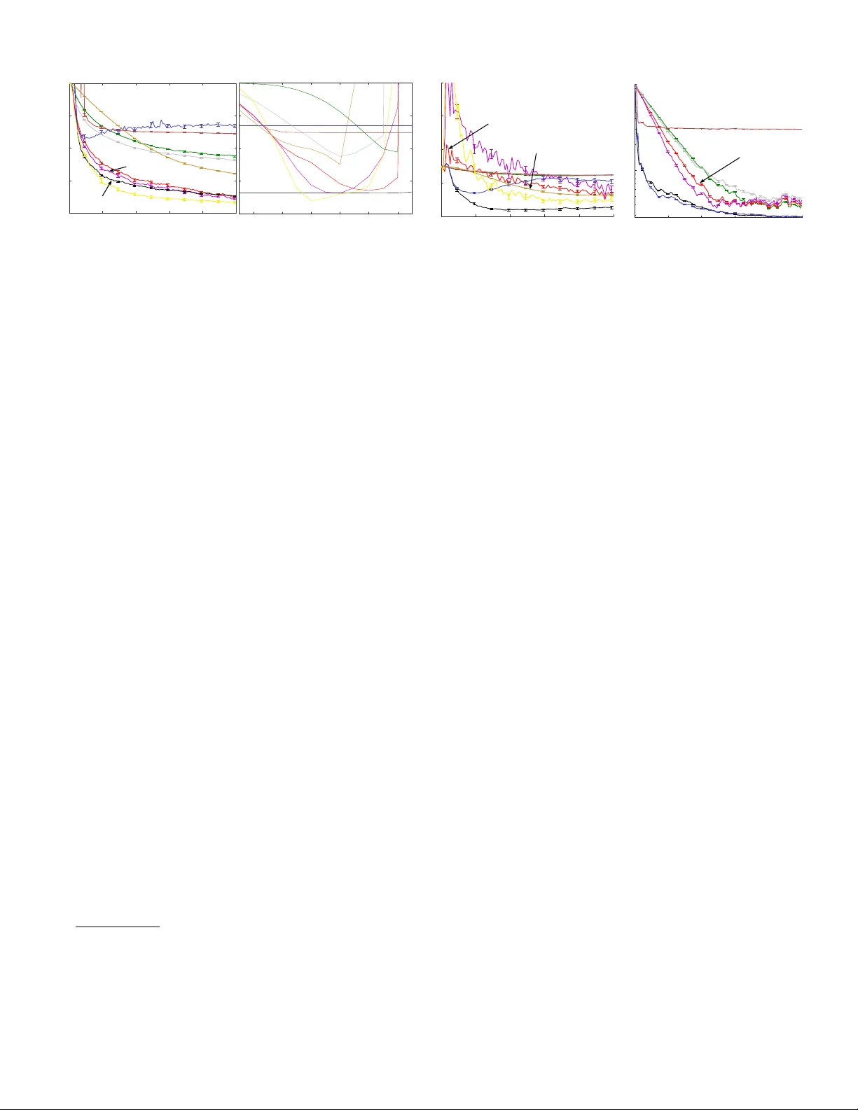
Accelerated Gradient T emporal Differ ence Learning Y angchen Pan, Adam White and Martha White Department of Computer Science Indiana Univ ersity at Bloomington {yangpan,adamw,martha}@indiana.edu Abstract The family of temporal dif ference (TD) methods span a spec- trum from computationally frugal linear methods like TD( λ ) to data efficient least squares methods. Least square methods make the best use of av ailable data directly computing the TD solution and thus do not require tuning a typically highly sensi- tiv e learning rate parameter , b ut require quadratic computation and storage. Recent algorithmic dev elopments have yielded sev eral sub-quadratic methods that use an approximation to the least squares TD solution, b ut incur bias. In this paper , we pro- pose a new family of accelerated gradient TD (A TD) methods that (1) provide similar data ef ficienc y benefits to least-squares methods, at a fraction of the computation and storage (2) sig- nificantly reduce parameter sensitivity compared to linear TD methods, and (3) are asymptotically unbiased. W e illustrate these claims with a proof of con vergence in e xpectation and experiments on se veral benchmark domains and a lar ge-scale industrial energy allocation domain. Introduction In reinforcement learning, a common strategy to learn an opti- mal policy is to iterativ ely estimate the v alue function for the current decision making policy—called policy evaluation — and then update the policy using the estimated values. The ov erall efficiency of this policy iteration scheme is directly in- fluenced by the efficienc y of the policy e v aluation step. T em- poral difference learning methods perform policy e v aluation: they estimate the v alue function directly from the sequence of states, actions, and rew ards produced by an agent interacting with an unknown en vironment. The family of temporal difference methods span a spec- trum from computationally-frugal, linear , stochastic approxi- mation methods to data ef ficient b ut quadratic least squares TD methods. Stochastic approximation methods, such as tem- poral difference (TD) learning (Sutton 1988) and gradient TD methods (Maei 2011) perform approximate gradient de- scent on the mean squared projected Bellman error (MSPBE). These methods require linear (in the number of features) computation per time step and linear memory . These lin- ear TD-based algorithms are well suited to problems with high dimensional feature vectors —compared to av ailable resources— and domains where agent interaction occurs at Copyright c  2017, Association for the Adv ancement of Artificial Intelligence (www .aaai.org). All rights reserved. a high rate (Szepesv ari 2010). When the amount of data is limited or difficult to acquire, the feature vectors are small, or data efficienc y is of primary concern, quadratic least squares TD (LSTD) methods may be preferred. These methods di- rectly compute the value function that minimizes the MSPBE, and thus LSTD computes the same v alue function to which linear TD methods con verge. Of course, there are many do- mains for which neither light weight linear TD methods, nor data efficient least squares methods may be a good match. Significant ef fort has focused on reducing the computation and storage costs of least squares TD methods in order to span the gap between TD and LSTD. The iLSTD method (Geram- ifard and Bo wling 2006) achie ves sub-quadratic computation per time step, b ut still requires memory that is quadratic in the size of the features. The tLSTD method (Gehring et al . 2016) uses an incremental singular v alue decomposition (SVD) to achiev e both sub-quadratic computation and storage. The ba- sic idea is that in many domains the update matrix in LSTD can be replaced with a low rank approximation. In practice tLSTD achiev es runtimes much closer to TD compared to iL- STD, while achieving better data efficienc y . A related idea is to use random projections to reduce computation and storage of LSTD (Gha v amzadeh et al . 2010). In all these approaches, a scalar parameter (descent dimensions, rank, and number of projections), controls the balance between computation cost and quality of solution. In this paper we explore a new approach called Accelerated gradient TD (A TD), that performs quasi-second-order gradi- ent descent on the MSPBE. Our aim is to dev elop a family of algorithms that can interpolate between linear TD methods and LSTD, without incurring bias. A TD, when combined with a lo w-rank approximation, con v er ges in expectation to the TD fixed-point, with con vergence rate dependent on the choice of rank. Unlike pre vious subquadratic methods, con- sistency is guaranteed ev en when the rank is chosen to be one. W e demonstrate the performance of A TD versus many linear and subquadratic methods in three domains, indicating that A TD (1) can match the data efficiency of LSTD, with signifi- cantly less computation and storage, (2) is unbiased, unlik e many of the alternativ e subquadratic methods, (3) signifi- cantly reduces parameter sensitivity for the step-size, v ersus linear TD methods, and (4) is significantly less sensitiv e to the choice of rank parameter than tLSTD, enabling a smaller rank to be chosen and so providing a more efficient incre- mental algorithm. Overall, the results suggest that A TD may be the first practical subquadratic complexity TD method suitable for fully incremental policy e v aluation. Background and Pr oblem F ormulation In this paper we focus on the problem of policy evaluation , or that of learning a v alue function gi v en a fixed polic y . W e model the interaction between an agent and its en vironment as a Marko v decision process ( S , A , P , r ) , where S denotes the set of states, A denotes the set of actions, and P : S × A × S → [0 , ∞ ) encodes the one-step state transition dynamics. On each discrete time step t = 1 , 2 , 3 , ... , the agent selects an action according to its behavior policy , A t ∼ µ ( S t , · ) , with µ : S × A → [0 , ∞ ) and the en vironment responds by transitioning into a new state S t +1 according to P , and emits a scalar rew ard R t +1 def = r ( S t , A t , S t +1 ) . The objective under policy ev aluation is to estimate the value function , v π : S → R , as the e xpected return from each state under some tar get policy π : S × A → [0 , ∞ ) : v π ( s ) def = E π [ G t | S t = s ] , where E π denotes the expectation, defined ov er the future states encountered while selecting actions according to π . The return , denoted by G t ∈ R is the discounted sum of future rew ards gi ven actions are selected according to π : G t def = R t +1 + γ t +1 R t +2 + γ t +1 γ t +2 R t +3 + ... (1) = R t +1 + γ t +1 G t +1 where γ t +1 ∈ [0 , 1] is a scalar that depends on S t , A t , S t +1 and discounts the contribution of future rew ards exponentially with time. The generalization to transition-based discount- ing enables the unification of episodic and continuing tasks (White 2016) and so we adopt it here. In the standard continu- ing case, γ t = γ c for some constant γ c < 1 and for a standard episodic setting, γ t = 1 until the end of an episode, at which point γ t +1 = 0 , ending the infinite sum in the return. In the most common on-policy ev aluation setting π = µ , otherwise π 6 = µ and policy e v aluation problem is said to be off-policy . In domains where the number of states is too large or the state is continuous, it is not feasible to learn the value of each state separately and we must generalize values between states using function approximation. In the case of linear func- tion approximation the state is represented by fixed length feature vectors x : S → R d , where x t def = x ( S t ) and the approximation to the value function is formed as a linear combination of a learned weight vector , w ∈ R d , and x ( S t ) : v π ( S t ) ≈ w > x t . The goal of policy e v aluation is to learn w from samples generated while following µ . The objecti ve we pursue towards this goal is to minimize the mean-squared projected Bellman error (MSPBE): MSPBE ( w , m ) = ( b m − A m w ) > C − 1 ( b m − A m w ) (2) where m : S → [0 , ∞ ) is a weighting function, A m def = E µ [ e m,t ( x t − γ t +1 x t +1 ) > ] b m def = E µ [ R t +1 e m,t ] C is an y positiv e definite matrix, typically C = E µ [ x t x > t ] with b m − A m w = E µ [ δ t ( w ) e m,t ] for TD-error δ t ( w ) = R t +1 + γ t +1 x > t +1 w − x > t w . The vector e m,t is called the eligibility trace e m,t def = ρ t ( γ t +1 λ e m,t − 1 + M t x t )  ρ t def = π ( s t , a t ) µ ( s t , a t ) M t s.t. E µ [ M t | S t = s t ] = m ( s ) /d µ ( s ) if d µ ( s ) 6 = 0 . where λ ∈ [0 , 1] is called the trace-decay parameter and d µ : S → [0 , ∞ ) is the stationary distribution induced by following µ . The importance sampling ratio ρ t reweights samples generated by µ to gi ve an e xpectation o ver π E µ [ δ t ( w ) e m,t ] = X s ∈S d µ ( s ) E π [ δ t ( w )( γ λ e m,t − 1 + M t x t ) | S t = s ] . This re-weighting enables v π to be learned from samples generated by µ (under of f-policy sampling). The most well-studied weighting occurs when M t = 1 (i.e., m ( s ) = d µ ( s )) . In the on-policy setting, with µ = π , ρ t = 1 for all t and m ( s ) = d π ( s ) the w that minimizes the MSPBE is the same as the w found by the on-policy temporal dif ference learning algorithm called TD( λ ). More recently , a new emphatic weighting was introduced with the emphatic TD (ETD) algorithm, which we denote m ETD . This weighting includes long-term information about π (see (Sutton et al. 2016, Pg. 16)), M t = λ t + (1 − λ t ) F t  F t = γ t ρ t − 1 F t − 1 + 1 . Importantly , the A m ETD matrix induced by the emphatic weighting is positive semi-definite (Y u 2015; Sutton et al . 2016), which we will later use to ensure con v er gence of our algorithm under both on- and of f-policy sampling. The A d µ used by TD( λ ) is not necessarily positiv e semi-definite, and so TD( λ ) can div er ge when π 6 = µ (off-polic y). T wo common strategies to obtain the minimum w of this objecti ve are stochastic temporal difference techniques, such as TD( λ ) (Sutton 1988), or directly approximating the linear system and solving for the weights, such as in LSTD( λ ) (Boyan 1999). The first class constitute linear complexity methods, both in computation and storage, in- cluding the family of gradient TD methods (Maei 2011), true online TD methods (van Seijen and Sutton 2014; van Hasselt et al . 2014) and sev eral others (see (Dann et al . 2014; White and White 2016) for a more complete summary). On the other e xtreme, with quadratic computation and stor - age, one can approximate A m and b m incrementally and solve the system A m w = b m . Given a batch of t samples { ( S i , A i , S i +1 , R i +1 ) } t i =1 , one can estimate A m,t def = 1 t t X i =1 e m,i ( x i − γ x i +1 ) > b m,t def = 1 t t X i =1 e m,i R i +1 , and then compute solution w such that A m,t w = b m,t . Least-squares TD methods are typically implemented incre- mentally using the Sherman-Morrison formula, requiring O ( d 2 ) storage and computation per step. Our goal is to develop algorithms that interpolate between these two extremes, which we discuss in the ne xt section. Algorithm derivation T o derive the ne w algorithm, we first take the gradient of the MSPBE (in 2) to get − 1 2 ∇ w MSPBE ( w , m ) = A > m C − 1 E µ [ δ t ( w ) e m,t ] . (3) Consider a second order update by computing the Hessian: H = A > m C − 1 A > m . For simplicity of notation, let A = A m and b = b m . For in vertible A , the second-order update is w t +1 = w t − α t 2 H − 1 ∇ w MSPBE ( w , m ) = w t + α t ( A > C − 1 A ) − 1 A > C − 1 E µ [ δ t ( w ) e m,t ] = w t + α t A − 1 CA −> A > C − 1 E µ [ δ t ( w ) e m,t ] = w t + α t A − 1 E µ [ δ t ( w ) e m,t ] In fact, for our quadratic loss, the optimal descent direc- tion is A − 1 E µ [ δ t ( w ) e m,t ] with α t = 1 , in the sense that argmin ∆ w loss ( w t + ∆ w ) = A − 1 E µ [ δ t ( w ) e m,t ] . Comput- ing the Hessian and updating w requires quadratic computa- tion, and in practice quasi-Ne wton approaches are used that approximate the Hessian. Additionally , there have been re- cent insights that using approximate Hessians for stochastic gradient descent can in fact speed conv ergence (Schrau- dolph et al . 2007; Bordes et al . 2009; Mokhtari and Ribeiro 2014). These methods maintain an approximation to the Hes- sian, and sample the gradient. This Hessian approximation provides curv ature information that can significantly speed con v ergence, as well as reduce parameter sensiti vity to the step-size. Our objecti ve is to improve on the sample ef ficienc y of lin- ear TD methods, while av oiding both quadratic computation and asymptotic bias. First, we need an approximation ˆ A to A that provides useful curv ature information, but that is also sub-quadratic in storage and computation. Second, we need to ensure that the approximation, ˆ A , does not lead to a biased solution w . W e propose to achiev e this by approximating only A − 1 and sampling E µ [ δ t ( w ) e m,t ] = b − Aw using δ t ( w t ) e t as an unbiased sample. The proposed accelerated temporal difference learning update—which we call A TD( λ )—is w t +1 = w t + ( α t ˆ A † t + η I ) δ t e t with expected update w t +1 = w t + ( α t ˆ A † + η I ) E µ [ δ t ( w ) e m,t ] (4) with regularization η > 0 . If ˆ A is a poor approximation of A , or discards key information—as we will do with a low rank approximation— then updating using only b − ˆ Aw will result in a biased solution, as is the case for tLSTD (Gehring et al . 2016, Theorem 1). Instead, sampling b − Aw = E µ [ δ t ( w ) e m,t ] , as we sho w in Theorem 1, yields an unbiased solution, ev en with a poor approximation ˆ A . The regularization η > 0 is key to ensure this consistency , by providing a full rank preconditioner α t ˆ A † t + η I . Giv en the general form of A TD( λ ), the next question is how to approximate A . T wo natural choices are a diagonal approximation and a low-rank approximation. Storing and using a diagonal approximation would only require linear O ( d ) time and space. For a low-rank approximation ˆ A , of rank k , represented with truncated singular value decomposi- tion ˆ A = U k Σ k V > k , the storage requirement is O ( dk ) and the required matrix-vector multiplications are only O ( dk ) be- cause for any vector v , ˆ Av = U k Σ k ( V > k v ) , is a sequence of O ( dk ) matrix-vector multiplications. Exploratory e xper - iments revealed that the low-rank approximation approach significantly outperformed the diagonal approximation. In general, howe v er , many other approximations to A could be used, which is an important direction for A TD. W e opt for an incremental SVD, that previously proved ef fectiv e for incremental estimation in reinforcement learning (Gehring et al . 2016). The total computational complexity of the algorithm is O ( dk + k 3 ) for the fully incremental update to ˆ A and O ( dk ) for mini-batch updates of k samples. Notice that when k = 0 , the algorithm reduces exactly to TD ( λ ), where η is the step-size. On the other extreme, where k = d , A TD is equiv alent to an iterati v e form of LSTD( λ ). See the appendix for a further discussion, and implementation details. Con v ergence of A TD( λ ) As with previous con v er gence results for temporal difference learning algorithms, the first key step is to prove that the expected update con ver ges to the TD fixed point. Unlike previous proofs of con ver gence in expectation, we do not require the true A to be full rank. This generalization is important, because as shown pre viously , A is often low-rank, ev en if features are linearly independent (Bertsekas 2007; Gehring et al . 2016). Further , A TD should be more effecti v e if A is lo w-rank, and so requiring a full-rank A would limit the typical use-cases for A TD. T o get across the main idea, we first prove con v er gence of A TD with weightings that give positi v e semi-definite A m ; a more general proof for other weightings is in the appendix. Assumption 1. A is diagonalizable, that is, there exists in- vertible Q ∈ R d × d with normalized columns (eigen vectors) and diagonal Λ ∈ R d × d , Λ = diag( λ 1 , . . . , λ d ) , such that A = QΛQ − 1 . Assume the or dering λ 1 ≥ . . . ≥ λ d . Assumption 2. α ∈ (0 , 2) and 0 < η ≤ λ − 1 1 max(2 − α, α ) . Finally , we introduce an assumption that is only used to characterize the con ver gence rate. This condition has been previously used (Hansen 1990; Gehring et al . 2016) to en- force a lev el of smoothness on the system. Assumption 3. The linear system defined by A = QΛQ − 1 and b satisfy the discr ete Picar d condition: for some p > 1 , | ( Q − 1 b ) j | ≤ λ p j for all j = 1 , . . . , rank ( A ) . Theorem 1. Under Assumptions 1 and 2, for any k ≥ 0 , let ˆ A be the rank- k appr oximation ˆ A = QΛ k Q − 1 of A m , wher e Λ k ∈ R d × d with Λ k ( j, j ) = λ j for j = 1 , . . . , k and zer o otherwise . If m = d µ or m ETD , the e xpected updating rule in (4) con ver ges to the fixed-point w ? = A † m b m . Further , if Assumption 3 is satisfied, the conver gence rate is k w t − w ? k ≤ max  max j ∈{ 1 ,...,k } | 1 − α − η λ j | t λ p − 1 j , max j ∈{ k +1 ,..., rank ( A ) } | 1 − η λ j | t λ p − 1 j  Proof: W e use a general result about stationary iterativ e methods which is applicable to the case where A is not full rank. Theorem 1.1 (Shi et al . 2011) states that gi ven a singular and consistent linear system Aw = b where b is in the range of A , the stationary iteration with w 0 ∈ R d for t = 1 , 2 , . . . w t = ( I − BA ) w t − 1 + Bb (5) con v erges to the solution w = A † b if and only if the follow- ing three conditions are satisfied. Condition I : the eigen v alues of I − BA are equal to 1 or hav e absolute v alue strictly less than 1. Condition II : rank ( BA ) = rank [( BA ) 2 ] . Condition III : nullspace ( BA ) = nullspace ( A ) . W e verify these conditions to prove the result. First, because we use the projected Bellman error, b is in the range of A and the system is consistent: there exists w s.t. Aw = b . T o rewrite our updating rule (4) to be expressible in terms of (5), let B = α ˆ A † + η I , giving BA = α ˆ A † A + η A = α QΛ † k Q − 1 QΛQ − 1 + η QΛQ − 1 = α QI k Q − 1 + η QΛQ − 1 = Q ( α I k + η Λ ) Q − 1 (6) where I k is a diagonal matrix with the indices 1 , . . . , k set to 1, and the rest zero. Proof for condition I . Using (6) , I − BA = Q ( I − α I k − η Λ ) Q − 1 . T o bound the maximum ab- solute value in the diagonal matrix I − α I k − η Λ , we consider eigen v alue λ j in Λ , and address two cases. Because A m is positiv e semi-definite for the assumed m (Sutton et al. 2016), λ j ≥ 0 for all j = 1 , . . . , d . Case 1: j ≤ k . | 1 − α − η λ j |  for 0 < η < max  2 − α λ 1 , α λ 1  < max( | 1 − α | , | 1 − α − (2 − α ) | , | 1 − α − α | ) = max( | 1 − α | , 1 , 1) < 1  because α ∈ (0 , 2) . Case 2: j > k . | 1 − η λ j | < 1 if 0 < η < 2 /λ j which is true for η = λ − 1 1 max(2 − α , α ) for any α ∈ (0 , 2) . Proof f or condition II. ( BA ) 2 does not change the number of positiv e eigen values, so the rank is unchanged. Proof for condition III . T o show the nullspaces of BA and A are equal, it is sufficient to prove BAw = 0 if and only if Aw = 0 . B = Q ( α Λ k + η I ) Q − 1 , is inv ertible because η > 0 and λ j ≥ 0 . For any w ∈ nullspace ( A ) , we get BAw = B0 = 0 , and so w ∈ nullspace ( BA ) . For an y w ∈ nullspace ( BA ) , BAw = 0 = ⇒ Aw = B − 1 0 = 0 , and so w ∈ nullspace ( A ) . Con ver gence rate. Assume w 0 = 0 . On each step, we up- date with w t +1 = ( I − BA ) w t + Bb = P t − 1 i =0 ( I − BA ) i Bb . This can be verified inducti v ely , where w t +1 = ( I − BA ) t − 2 X i =0 ( I − BA ) i Bb + ( I − BA ) 0 Bb = t − 1 X i =0 ( I − BA ) i Bb . For ¯ Λ = I − α I k − η Λ , because ( I − BA ) i = Q ¯ Λ i Q − 1 , w t = Q t − 1 X i =0 ¯ Λ i ! Q − 1 Q ( α Λ † k + η I ) Q − 1 b = Q t − 1 X i =0 ¯ Λ i ! ( α Λ † k + η I ) Q − 1 b and because w t → w ? , k w t − w ? k = k Q ∞ X i =0 ¯ Λ i − t X i =0 ¯ Λ i ! ( α Λ † k + η I ) Q − 1 b k = k Q ¯ Λ t ( α Λ † k + η I ) Q − 1 b k  ¯ Λ t ( j, j ) def = ¯ λ t j 1 − ¯ λ j ≤ k Q kk ¯ Λ t ( α Λ † k + η I ) Q − 1 b k where k Q k ≤ 1 because Q has normalized columns. For j = 1 , . . . , k , we hav e that the magnitude of the values in ¯ Λ t ( α Λ † k + η I ) are (1 − α − η λ j ) t α + η λ j ( αλ − 1 j + η ) = (1 − α − η λ j ) t λ j . For j = k , . . . , rank ( A ) , we get (1 − η λ j ) t λ j . Under the discrete Picard condition, | ( Q − 1 b ) j | ≤ λ p j and so the denominator λ j cancels, giving the desired result.  This theorem giv es insight into the utility of A TD for speed- ing con v ergence, as well as the effect of k . Consider TD( λ ), which has positi ve definite A in on-policy learning (Sutton 1988, Theorem 2). The abov e theorem guarantees A TD con- ver gences to the TD fixed-point, for any k . For k = 0 , the expected A TD update is exactly the expected TD update. Now , we can compare the conv er gence rate of TD and A TD, using the abov e con v er gence rate. T ake for instance the setting α = 1 for A TD, which is com- mon for second-order methods and let p = 2 . The rate of con- ver gence reduces to the maximum of max j ∈{ 1 ,...,k } η t λ t +1 j and max j ∈{ k +1 ,..., rank ( A ) } | 1 − η λ j | t λ j . In early learning, the con v ergence rate for TD is dominated by | 1 − η λ 1 | t λ 1 , be- cause λ j is largest relati v e to | 1 − η λ j | t for small t . A TD, on the other hand, for a larger k , can pick a smaller η and so has a much smaller v alue for j = 1 , i.e., η t λ t +1 1 , and | 1 − η λ j | t λ j is small because λ j is small for j > k . As k gets smaller, | 1 − η λ k +1 | t λ k +1 becomes larger , slowing con vergence. F or low-rank domains, howe ver , k could be quite small and the preconditioner could still improve the conv ergence rate in early learning—potentially significantly outperforming TD. A TD is a quasi-second order method, meaning sensitivity to parameters should be reduced and thus it should be simpler to set the parameters. The con v er gence rate provides intuition that, for reasonably chosen k , the regularizer η should be small—smaller than a typical stepsize for TD. Additionally , because A TD is a stochastic update, not the expected update, we make use of typical con v entions from stochastic gradient descent to set our parameters. W e set α t = α 0 t , as in pre vious stochastic second-order methods (Schraudolph et al . 2007), where we choose α 0 = 1 and set η to a small fixed v alue. Our choice for η represents a small final step-size, as well as matching the con v ergence rate intuition. On the bias of subquadratic methods. The A TD( λ ) up- date was deri v ed to ensure con vergence to the minimum of the MSPBE, either for the on-polic y or of f-polic y setting. Our algorithm summarizes past information, in ˆ A , to improv e the con v ergence rate, without requiring quadratic computation and storage. Prior work aspired to the same goal, howe ver , the resultant algorithms are biased. The iLSTD algorithm can be shown to con ver ge for a specific class of feature selec- tion mechanisms (Geramifard et al . 2007, Theorem 2); this class, ho we ver , does not include the greedy mechanism that is used in iLSTD algorithm to select a descent direction. The random projections variant of LSTD (Ghav amzadeh et al . 2010) can significantly reduce the computational complexity compared with con v entional LSTD, with projections down to size k , but the reduction comes at a cost of an increase in the approximation error (Gha vamzadeh et al . 2010). Fast LSTD (Prashanth et al . 2013) does randomized TD updates on a batch of data; this algorithm could be run incrementally with O( dk ) by using mini-batches of size k . Though it has a nice theoretical characterization, this algorithm is restricted to λ = 0 . Finally , the most related algorithm is tLSTD, which also uses a low-rank approximation to A . In A TD ˆ A t is used very differently , from how ˆ A t is used in tLSTD. The tLSTD algorithm uses a similar approxima- tion ˆ A t as A TD, but tLSTD uses it to compute a closed form solution w t = ˆ A † t b t , and thus is biased (Gehring et al . 2016, Theorem 1). In f act, the bias gro ws with decreasing k , propor - tionally to the magnitude of the k th largest singular v alue of A . In A TD, the choice of k is decoupled from the fixed point, and so can be set to balance learning speed and computation with no fear of asymptotic bias. Empirical Results All the follo wing e xperiments in v estigate the on-polic y set- ting, and thus we make use of the standard v ersion of A TD for simplicity . Future work will explore off-policy domains with the emphatic update. The results presented in this section were generated ov er 756 thousand individual experiments run on three different domains. Due to space constraints detailed descriptions of each domain, error calculation, and all other parameter settings are discussed in detail in the appendix. W e included a wide variety of baselines in our experiments, additional related baselines excluded from our study are also discussed in the appendix. 1 2 3 4 5 6 7 8 9 10 11 12 13 14 15 16 17 18 0 0.1 0.2 0.3 0.4 0.5 1 2 3 4 5 6 7 8 9 10 11 12 13 14 15 16 17 18 Alpha/N 0 0.1 0.2 0.3 0.4 0.5 PAME TD(0) LSTD A TD ETD T0ETD TOTD TD( λ ) TD(0) ETD TD( λ ) TOTD T0ETD 𝛂 / η 𝛂 / η with n 0 =10 2 𝛂 / η with n 0 =10 6 Cons t ant s tep-size Deca y ed s tep-size per cent ag e er r or per cent ag e er r or Figure 1: Parameter sensitivity in Boyan’ s chain with constant step-size (LHS) and decayed step-sizes (RHS). In the plots abo ve, each point summarizes the mean performance (over 1000 time steps) of an algorithm for one setting of α for linear methods, or η for LSTD, and α/ 100 regularizer for A TD, using percentage error compared to the true v alue function. In the decayed step-size case, where α t = α 0 n 0 +1 n 0 + episode# , 18 values of α 0 and two values of n 0 were tested—corresponding to the two sides of the RHS graph. The LSTD algorithm (in yello w) has no parameters to decay . Our A TD algorithm (in black) achie ves the lo west error in this domain, and exhibits little sensitivity to it’ s regularization parameter (with step-size as α t = 1 t across all experiments). Our first batch of experiments were conducted on Boyan’ s chain—a domain kno wn to elicit the strong advantages of LSTD( λ ) ov er TD( λ ). In Boyan’ s chain the agent’ s objecti ve is to estimate the value function based on a low-dimensional, dense representation of the underlying state (perfect represen- tation of the value function is possible). The ambition of this experiment w as to in vestigate the performance of A TD in a domain where the pre-conditioner matrix is full rank; no rank truncation is applied. W e compared fi ve linear-comple xity methods (TD(0), TD( λ ), true online TD( λ ), ETD( λ ), true online ETD( λ )), against LSTD( λ ) and A TD, reporting the percentage error relati ve to the true v alue function o v er the first 1000 steps, averaged over 200 independent runs. W e swept a lar ge range of step-size parameters, trace decay rates, and regularization parameters, and tested both fixed and de- caying step-size schedules. Figure 1 summarizes the results. Both LSTD( λ ) and A TD achiev e lower error compared to all the linear baselines—ev en thought each linear method was tuned using 864 combinations of step-sizes and λ . In terms of sensitivity , the choice of step-size for TD(0) and ETD exhibit lar ge effect on performance (indicated by sharp valle ys), whereas true-online TD( λ ) is the least sensiti v e to learning rate. LSTD( λ ) using the Sherman-Morrison update (used in many prior empirical studies) is sensitiv e to the regularization parameter; the parameter free nature of LSTD may be slightly ov erstated in the literature. 1 Our second batch of experiments inv estigated character- istics of A TD in a classic benchmark domain with a sparse high-dimensional feature representation where perfect ap- proximation of the value function is not possible—Mountain car with tile coding. The polic y to be e v aluated stochastically takes the action in the direction of the sign of the velocity , with performance measured by computing a truncated Monte 1 W e are not the first to observe this. Sutton and Barto (2016) note that η plays a role similar to the step-size for LSTD. 1000 2000 3000 4000 5000 0.2 0.4 0.6 0.8 1 2 4 6 8 10 12 0 .2 0 .4 0 .6 0 .8 1 percentage error time steps tLSTD RP-LSTD iLSTD TD(0) fast LSTD LSTD AT D TO-TD TO-ETD AT D LSTD tLSTD p e rce n t a g e e rro r 𝛂 / η rank = 50 Figure 2: The learning curv es (LHS) are percentage error v ersus time steps av eraged ov er 100 runs of A TD with rank 50, LSTD and sev eral baselines described in text. The sensitivity plot (RHS) is with respect to the learning rate of the linear methods, and re gular- ization parameter of the matrix methods. The tLSTD algorithm has no parameter besides rank, while A TD has little sensiti vity to it’ s regularization parameter . Carlo estimate of the return from states sampled from the stationary distribution (detailed in the appendix). W e used a fine grain tile coding of the the 2D state, resulting in a 1024 dimensional feature representation with e xactly 10 units acti ve on e very time step. W e tested TD(0), true online TD( λ ) true online ETD( λ ), and sub-quadratic methods, including iLSTD, tLSTD, random projection LSTD, and fast LSTD (Prashanth et al . 2013). As before a wide range of parameters ( α, λ, η ) were swept ov er a lar ge set. Performance was a v er - aged ov er 100 independent runs. A fix ed step-size schedule was used for the linear TD baselines, because that achiev ed the best performance. The results are summarized in figure 2. LSTD and A TD exhibit faster initial learning compared to all other methods. This is particularly impressive since k is less than 5% of the size of A . Both fast LSTD and projected LSTD perform considerably worse than the linear TD-methods, while iLSTD exhibits high parameter sensiti v- ity . tLSTD has no tunable parameter besides k , but performs poorly due to the high stochasticity in the policy—additional experiments with randomness in action selection of 0% and 10% yielded better performance for tLSTD, b ut ne ver equal to A TD. The true online linear methods perform very well compared to A TD, but this required sweeping hundreds of combinations of α and λ , whereas A TD exhibited little sen- sitivity to it’ s regularization parameter (see Figure 2 RHS); A TD achieved e xcellent performance with the same parame- ter setting as we used in Boyan’ s chain. 2 W e ran an additional experiment in Mountain car to more clearly exhibit the benefit of A TD over e xisting methods. W e used the same setting as above, except that 100 additional features were added to the feature vector , with 50 of them randomly set to one and the rest zero. This noisy feature vector is meant to emulate a situation such as a robot that has a sensor that becomes unreliable, generating noisy data, b ut the remaining sensors are still useful for the task at hand. The results are summarized in Figure 4. Naturally all methods are adversely effected by this change, howe v er A TD’ s low 2 For the remaining experiments in the paper, we excluded the TD methods without true online traces because they perform worse than their true online counterparts in all our experiments. This result matches the results in the literature (van Seijen et al. 2016). 2000 4000 6000 8000 10000 10 -1 10 0 1000 2000 3000 4000 5000 0.4 0.8 1.2 1.6 2 percentage error time steps tLSTD iLSTD TD(0) / R-LSTD / F-LSTD LSTD TO-TD TO-ETD AT D Mountain Car w noisy features time steps RP-LSTD TD(0) fast-LSTD TO-ETD tLSTD AT D TO-TD Energy domain Figure 3: Learning curves on Mountain Car with noisy features (LHS) and on Energy allocation (RHS), in logscale. rank approximation enables the agent to ignore the unreliable feature information and learn efficiently . tLSTD, as suggested by our pre vious experiments does not seem to cope well with the increase in stochasticity . Our final experiment compares the performance of several sub-quadratic complexity policy e v aluation methods in an in- dustrial energy allocation simulator with much larger feature dimension (see Figure 4). As before we report percentage error computed from Monte Carlo rollouts, averaging perfor - mance over 50 independent runs and selecting and testing parameters from an extensi v e set (detailed in the appendix). The policy was optimized ahead of time and fixed, and the feature vectors were produced via tile coding, resulting in an 8192 dimensional feature vector with 800 units active on each step. Although the feature dimension here is still relativ ely small, a quadratic method like LSTD nonetheless would require o ver 67 million operations per time step, and thus methods that can exploit low rank approximations are of particular interest. The results indicate that both A TD and tLSTD achiev e the fastest learning, as e xpected. The instrin- sic rank in this domain appears to be small compared to the feature dimension—which is exploited by A TD and tLSTD with r = 40 —while the performance of tLSTD indicates that the domain exhibits little stochasticity . The appendix contains additional results for this domain—in the small rank setting A TD significantly outperforms tLSTD. Conclusion and future w ork In this paper , we introduced a new family of TD learning algorithms that take a fundamentally dif ferent approach from previous incremental TD algorithms. The ke y idea is to use a preconditioner on the temporal dif ference update, similar to a quasi-Ne wton stochastic gradient descent update. W e prov e that the e xpected update is consistent, and empirically demon- strated improv ed learning speed and parameter insensiti vity , ev en with significant approximations in the preconditioner . This paper only begins to scratch the surface of poten- tial preconditioners for A TD. There remains many a v enues to explore the utility of other preconditioners, such as di- agonal approximations, eigen v alues estimates, other matrix factorizations and approximations to A that are amenable to in v ersion. The family of A TD algorithms provides a promis- ing avenue for more effecti v ely using results for stochastic gradient descent to improve sample complexity , with feasible computational complexity . References [Bertsekas 2007] Bertsekas, D. 2007. Dynamic Pr ogramming and Optimal Contr ol . Athena Scientific Press. [Bordes et al. 2009] Bordes, A.; Bottou, L.; and Gallinari, P . 2009. SGD-QN: Careful quasi-Newton stochastic gradient descent. Journal of Machine Learning Resear ch . [Boyan 1999] Boyan, J. A. 1999. Least-squares temporal difference learning. International Confer ence on Machine Learning . [Dabney and Thomas 2014] Dabney , W ., and Thomas, P . S. 2014. Natural T emporal Difference Learning. In AAAI Con- fer ence on Artificial Intelligence . [Dann et al. 2014] Dann, C.; Neumann, G.; and Peters, J. 2014. Policy e v aluation with temporal dif ferences: a surv ey and comparison. The Journal of Mac hine Learning Resear ch . [Gehring et al. 2016] Gehring, C.; Pan, Y .; and White, M. 2016. Incremental Truncated LSTD. In International Joint Confer ence on Artificial Intelligence . [Geramifard and Bo wling 2006] Geramifard, A., and Bowl- ing, M. 2006. Incremental least-squares temporal difference learning. In AAAI Conference on Artificial Intellig ence . [Geramifard et al. 2007] Geramifard, A.; Bowling, M.; and Zinke vich, M. 2007. iLSTD: Eligibility traces and conv er- gence analysis. In Advances in Neural Information Pr ocess- ing Systems . [Ghav amzadeh et al. 2010] Ghav amzadeh, M.; Lazaric, A.; Maillard, O. A.; and Munos, R. 2010. LSTD with random projections. In Advances in Neural Information Pr ocessing Systems . [Givchi and P alhang 2014] Givc hi, A., and Palhang, M. 2014. Quasi newton temporal dif ference learning. In Asian Confer- ence on Machine Learning . [Hansen 1990] Hansen, P . C. 1990. The discrete picard con- dition for discrete ill-posed problems. BIT Numerical Mathe- matics . [Maei 2011] Maei, H. 2011. Gradient T emporal-Dif fer ence Learning Algorithms . Ph.D. Dissertation, Univ ersity of Al- berta. [Mahadev an et al. 2014] Mahadev an, S.; Liu, B.; Thomas, P . S.; Dabney , W .; Giguere, S.; Jacek, N.; Gemp, I.; and 0002, J. L. 2014. Proximal reinforcement learning: A new theory of sequential decision making in primal-dual spaces. CoRR abs/1405.6757 . [Meyer et al. 2014] Meyer , D.; Degenne, R.; Omrane, A.; and Shen, H. 2014. Accelerated gradient temporal difference learning algorithms. In IEEE Symposium on Adaptive Dy- namic Pr o gramming and Reinfor cement Learning . [Mokhtari and Ribeiro 2014] Mokhtari, A., and Ribeiro, A. 2014. RES: Regularized stochastic BFGS algorithm. IEEE T ransactions on Signal Pr ocessing . [Prashanth et al. 2013] Prashanth, L. A.; K orda, N.; and Munos, R. 2013. Fast LSTD using stochastic approximation: Finite time analysis and application to traffic control. ECML PKDD . [Salas and Powell 2013] Salas, D. F ., and Po well, W . B. 2013. Benchmarking a Scalable Approximate Dynamic Program- ming Algorithm for Stochastic Control of Multidimensional Energy Storage Problems. Dept Oper Res Financial Eng . [Schraudolph et al. 2007] Schraudolph, N.; Y u, J.; and Gün- ter , S. 2007. A stochastic quasi-Newton method for online con v ex optimization. In International Conference on Artifi- cial Intelligence and Statistics . [Shi et al. 2011] Shi, X.; W ei, Y .; and Zhang, W . 2011. Con- ver gence of general nonstationary iterati ve methods for solv- ing singular linear equations. SIAM Journal on Matrix Anal- ysis and Applications . [Sutton and Barto 1998] Sutton, R., and Barto, A. G. 1998. Reinfor cement Learning: An Intr oduction . MIT press. [Sutton and Barto 2016] Sutton, R., and Barto, A. G. 2016. Reinfor cement Learning: An Intr oduction 2nd Edition . MIT press. [Sutton et al. 2016] Sutton, R. S.; Mahmood, A. R.; and White, M. 2016. An emphatic approach to the problem of off-policy temporal-difference learning. The Journal of Machine Learning Resear ch . [Sutton 1988] Sutton, R. 1988. Learning to predict by the methods of temporal differences. Machine Learning . [Szepesvari 2010] Szepesvari, C. 2010. Algorithms for Rein- for cement Learning . Morgan & Claypool Publishers. [van Hasselt et al. 2014] van Hasselt, H.; Mahmood, A. R.; and Sutton, R. 2014. Off-polic y TD ( λ ) with a true on- line equi valence. In Conference on Uncertainty in Artificial Intelligence . [van Seijen and Sutton 2014] van Seijen, H., and Sutton, R. 2014. True online TD(lambda). In International Conference on Machine Learning . [van Seijen et al. 2016] van Seijen, H.; Mahmood, R. A.; Pi- larski, P . M.; Machado, M. C.; and Sutton, R. S. 2016. True Online T emporal-Difference Learning. In Journal of Machine Learning Resear c h . [W ang and Bertsekas 2013] W ang, M., and Bertsekas, D. P . 2013. On the con vergence of simulation-based iterative meth- ods for solving singular linear systems. Stochastic Systems . [White and White 2016] White, A. M., and White, M. 2016. In v estigating practical, linear temporal dif ference learning. In International Confer ence on Autonomous Agents and Mul- tiagent Systems . [White 2016] White, M. 2016. Unifying task specification in reinforcement learning. arXiv .org . [Y u 2015] Y u, H. 2015. On con vergence of emphatic temporal-difference learning. In Annual Confer ence on Learning Theory . Con v ergence pr oof For the more general setting, where m can also equal D µ , we redefine the rank- k approximation. W e say the rank- k approximation ˆ A to A is composed of eigenv alues { λ i 1 , . . . , λ i k } ⊆ { λ 1 , . . . , λ d } if ˆ A = QΛ k Q − 1 for diago- nal Λ k ∈ R d × d , Λ ( i j , i j ) = λ i j for j = 1 , . . . , k , and zero otherwise. Theorem 2. Under Assumptions 1 and 2, let ˆ A be the r ank- k appr oximation composed of eigen values { λ i 1 , . . . , λ i k } ⊆ { λ 1 , . . . , λ d } . If λ d ≥ 0 or { λ i 1 , . . . , λ i k } contains all the ne gative eig en values in { λ 1 , . . . , λ d } , then the e xpected up- dating rule in (4) con ver ges to the fixed-point w ? = A † b . Proof: W e use a general result about stationary iterativ e methods (Shi et al . 2011), which is applicable to the case where A is not full rank. Theorem 1.1 (Shi et al . 2011) states that gi ven a singular and consistent linear system Aw = b where b is in the range of A , the stationary iteration with w 0 ∈ R d for t = 1 , 2 , . . . w i = ( I − BA ) w t − 1 + Bb (5) con v erges to the solution w = A † b if and only if the follow- ing three conditions are satisfied. Condition I : the eigen v alues of I − BA are equal to 1 or hav e absolute v alue strictly less than 1. Condition II : rank ( BA ) = rank [( BA ) 2 ] . Condition III : the null space N ( BA ) = N ( A ) . W e verify these conditions to prove the result. First, because we are using the projected Bellman error , we kno w that b is in the range of A and the system is consistent: there exists w s.t. Aw = b . T o rewrite our updating rule (4) to be expressible in terms of (5), let B = α ˆ A † + η I , giving BA = α ˆ A † A + η A = α QΛ † k Q − 1 QΛQ − 1 + η QΛQ − 1 = α QI k Q − 1 + η QΛQ − 1 = Q ( α I k + η Λ ) Q − 1 (6) where I k is a diagonal matrix with the indices i 1 , . . . , i k set to 1, and the rest zero. Proof for condition I . Using (6) , I − BA = Q ( I − α I k − η Λ ) Q − 1 . T o bound the maximum ab- solute value in the diagonal matrix I − α I k − η Λ , we consider eigen v alue λ j in Λ , and address three cases. Case 1: j ∈ { i 1 , . . . , i k } , λ j ≥ 0 : | 1 − α − η λ j |  for 0 < η < max  2 − α λ 1 , α λ 1  < max( | 1 − α | , | 1 − α − (2 − α ) | , | 1 − α − α | ) = max( | 1 − α | , 1 , 1) < 1  because α ∈ (0 , 2) . Case 2: j ∈ { i 1 , . . . , i k } , λ j < 0 : | 1 − α − η λ i | = | 1 − α + η | λ i || < 1 if 0 ≤ 1 − α + η | λ i | < 1 = ⇒ η < α/ | λ i | . Case 3: j / ∈ { i 1 , . . . , i k } . For this case, λ j ≥ 0 , by as- sumption, as { i 1 , . . . , i k } contains the indices for all negati ve eigen v alues of A . So | 1 − η λ i | < 1 if 0 < η < 2 /λ i . All three cases are satisfied by the assumed α ∈ (0 , 2) and η ≤ λ − 1 max max(2 − α, α ) . Therefore, the absolute v alue of the eigen v alues of I − BA are all less than 1 and so the first condition holds. Proof for condition II. ( BA ) 2 does not change the number of positiv e eigen values, so the rank is unchanged. BA = Q ( α I k + η Λ ) Q − 1 ( BA ) 2 = Q ( α I k + η Λ ) Q − 1 Q ( α I k + η Λ ) Q − 1 = Q ( α I k + η Λ ) 2 Q − 1 Proof f or condition III . T o show that the nullspaces of BA and A are equal, it is sufficient to prove BAw = 0 if and only if Aw = 0 . Because B = Q ( α Λ k + η I ) Q − 1 , we kno w that B is in vertible as long as α 6 = − η λ j . Because η > 0 , this is clearly true for λ j ≥ 0 and also true for λ j < 0 because η is strictly less than α/ | λ j | . For any w ∈ nullspace ( A ) , we get BAw = B0 = 0 , and so w ∈ nullspace ( BA ) . For any w ∈ nullspace ( BA ) , we get BAw = 0 = ⇒ Aw = B − 1 0 = 0 , and so w ∈ nullspace ( A ) , completing the proof.  W ith k = d , the update is a gradient descent update on the MSPBE, and so will con v erge ev en under off-polic y sampling. As k << d , the gradient is only approximate and theoretical results about (stochastic) gradient descent no longer obvi- ously apply . For this reason, we use the iterativ e update anal- ysis abov e to understand conv er gence properties. Iterative updates for the full expected update, with preconditioners, hav e been studied in reinforcement learning (c.f. (W ang and Bertsekas 2013)); howe v er , the y typically analyzed dif ferent preconditioners, as they had no requirements for reducing computation belo w quadratic computation. For e xample, they consider a regularized preconditioner B = ( A + η I ) − 1 , which is not compatible with an incremental singular value decomposition and, to the best of our knowledge, current iter- ativ e eigen value decompositions require symmetric matrices. The theorem is agnostic to what components of A are approximated by the rank- k matrix ˆ A . In general, a natural choice, particularly in on-policy learning or more generally with a positi ve definite A , is to select the largest magnitude eigen v alues of A , which contain the most significant informa- tion about the system and so are likely to giv e the most useful curvature information. Ho we v er , ˆ A could also potentially be chosen to obtain conv er gence for off-polic y learning with m = d µ , where A is not necessarily positiv e semi-definite. This theorem indicates that if the rank k approximation ˆ A contains the negati v e eigenv alues of A , e ven if it does not contain the remaining information in A , then we obtain con- ver gence under off-policy sampling. W e can of course use the emphatic weighting more easily for off-policy learning, but if the weighting m = d µ is desired rather than m ETD , then carefully selecting ˆ A for A TD enables that choice. Algorithm 1 Accelerated T emporal Difference Learning  where U 0 = [] , V 0 = [] , Σ 0 = [] , b 0 = 0 , e 0 = 0 , initialized w 0 arbitrarily function A T D( k , η , λ ) x 0 = first observation η = a small final stepsize value, e.g., η = 10 e − 4 for t = 0 , 1 , 2 , ... do In x t , select action A t ∼ π , observe x t +1 , rew ard r t +1 , discount γ t +1 (could be zero if terminal state) β t = 1 / ( t + 1) δ t = r t +1 + γ t +1 w > x t +1 − w > x t e t = T R A C E _ U P DA T E ( e t − 1 , x t , γ t , λ t )  or call E M PA H T I C _ T R AC E _ U P DAT E to use emphatic weighting  U t Σ t V > t = (1 − β t ) U t − 1 Σ t − 1 V > t − 1 + β t e t ( x t − γ t +1 x t +1 ) > [ U t , Σ t , V t ] = S V D - U P DAT E ( U t − 1 , (1 − β t ) Σ t − 1 , V t − 1 , √ β t e t , √ β t ( x t − γ t +1 x t +1 ) , k )  see (Gehring et al . 2016)  Ordering of matrix operations important, first multiply U > t e t in O ( dk ) time  to get a new vector , then by Σ † t and V t to maintain only matrix-vector multiplications w t +1 = w t + ( 1 t +1 V t Σ † t U > t + η I )( δ t e t )  where Σ † t = diag( ˆ σ − 1 1 , . . . , ˆ σ − 1 k , 0 ) Algorithmic details In this section, we outline the implemented A TD( λ ) algo- rithm. The key choices are ho w to update the approximation to ˆ A , and how to update the eligibility trace to obtain dif- ferent v ariants of TD. W e include both the conv entional and emphatic trace updates in Algorithms 2 and 3 respectiv ely . The lo w-rank update to ˆ A uses an incremental singular v alue decomposition (SVD). This update to ˆ A is the same one used for tLSTD, and so we refer the reader to (Gehring et al . 2016, Algorithm 3). The general idea is to incorporate the rank one update e t ( x t − γ t +1 x t +1 ) > into the current SVD of ˆ A . In addition, to maintain a normalized ˆ A , we multiply by β t : ˆ A t +1 = (1 − β t ) ˆ A + β t e t ( x t − γ t +1 x t +1 ) > = t t +1 ˆ A + 1 t +1 e t ( x t − γ t +1 x t +1 ) > Multiplying ˆ A by a constant corresponds to multiplying the singular values. W e also find that multiplying each compo- nent of the rank one update by p 1 / ( t + 1) is more effecti v e than multiplying only one of them by 1 / ( t + 1) . Algorithm 2 Con v entional trace update for A TD function T R A C E _ U P DA T E ( e t − 1 , x t , γ t , λ t ) retur n γ t λ t e t − 1 + x t Algorithm 3 Emphatic trace update for A TD  where F 0 ← 0 , M 0 ← 0 is initialized globally , before ex ecuting the for loop in A TD( λ ) function E M P H A T I C _ T R AC E _ U P DAT E ( e t − 1 , x t , γ t , λ t ) ρ t ← π ( s t ,a t ) µ ( s t ,a t )  Where ρ t = 1 in the on-policy case F t ← ρ t − 1 γ t F t − 1 + i t  For uniform interest, i t = 1 M t ← λ t i t + (1 − λ t ) F t retur n ρ t ( γ t λ t e t − 1 + M t x t ) Detailed experimental specification In both mountain car and energy storage domains we do not hav e access to the parameter’ s of the underlying MDPs (as we do in Boyan’ s chain), and thus must turn to Monte Carlo rollouts to estimate v π in order to e v aluate our v alue function approximation methods. In both domains we follo wed the same strategy . T o generate training data we generated 100 trajectories of rew ards and observ ations under the target polic y , starting in randomly from a small area near a start state. Each tra- jectory is composed of a fixed number of steps, either 5000 or 10000, and, in the case of episodic tasks like mountain car , may contain many episodes. The start states for each trajectory were sampled uniform randomly from (1) near the bottom of the hill with zero v elocity for mountain car , (2) a small set of v alid start states specified by the energy storage domains (Salas and Po well 2013). Each trajectory represents one independent run of the domain. The testing data was sampled according to the on-polic y distribution induced by the target policy . For both domains we generated a single long trajectory selecting actions according to π . Then we randomly sampled 2000 states from this one trajectory . In mountain car domain, we ran 500 Monte Carlo rollouts to compute undiscounted sum of future rewards until termination, and take the av erage as an estimate true v alue. In the energy allocation domain, we ran 300 Monte Carlo roll- outs for each e v aluation state, each with length 1000 steps 3 , av eraging o ver 300 trajectories from each of the ev aluation states. W e ev aluated the algorithms’ performances by compar- ing the agent’ s prediction value with the estimated value of the 2000 ev aluation states, at every 50 steps during training. W e measured the percentage absolution mean error: error ( w ) = 1 2000 2000 X i =1 | w T x ( s i ) − ˆ v π ( s i ) | | ˆ v π ( s i ) | , 3 After 1000 steps, for γ = 0 . 99 , the reward in the return is multiplied by γ 1000 < 10 − 5 and so contrib utes a ne gligible amount to the return. where ˆ v π ( s i ) ∈ R denotes the Monte Carlo estimate of the value of e v aluation state s i . Algorithms The algorithms included in the experiments constitute a wide range of stochastic approximation algorithms and matrix- based (subquadratic) algorithms. There are a few related algorithms, ho we ver , that we chose not to include; for com- pleteness we explain our decision making here. There hav e been some accelerations proposed to gradient TD algorithms (Mahadev an et al . 2014; Meyer et al . 2014; Dabney and Thomas 2014). Howe v er , they ha v e either shown to perform poorly in practice (White and White 2016), or were based on applying accelerations outside their intended use (Meyer et al . 2014; Dabney and Thomas 2014). Dabney and Thomas (2014) explored a similar update to A TD, but for the control setting and with an incremental update to the Fisher information matrix rather than A used here. As the y acknowledge, this approach for TD methods is somewhat adhoc, as the typical update is not a gradient, and rather their method is better suited for the policy gradient algorithms explored in that paper . Me yer et al . (2014) applied an acceler - ated Nesterov technique, called SA GE, to the two timescale gradient algorithms. Their approach does not take advantage of the simpler quadratic form of the MSPBE, and so only uses an approximate Lipschitz constant to improv e selection of the stepsize. Diagonal approximations to A constitute a strictly more informative stepsize approach, and we found these to be inferior to our low-rank strategy . The results by Meyer et al . (2014) using SA GE for GTD similarly indicated little to no gain. Finally , Givchi and Palhang (2014) adapted SGD-QN for TD, and showed some impro vements using this diagonal step-size approximation. On the other hand, the true-online methods hav e consis- tently been shown to ha v e surprisingly strong performance (White and White 2016), and so we opt instead for these practical competitors. Boyan’ s Chain This domain was implemented exactly as describe in Boyan’ s paper (Boyan 1999). The task is episodic and the true value function is known, and thus we did not need to compute rollouts. Otherwise e v aluation was performed e xactly as de- scribed abov e. W e tested the following parameter settings: • α 0 ∈ { 0 . 1 × 2 . 0 j | j = − 12 , − 11 , − 10 , ..., 4 , 5 } , 18 values in total • n 0 ∈ { 10 2 , 10 6 } • λ ∈ { 0 . 0 , 0 . 1 , ..., 0 . 9 , 0 . 91 , 0 . 93 , 0 . 95 , 0 . 97 , 0 . 99 , 1 . 0 } , 16 values in total • η ∈ { 10 j | j = − 4 , − 3 . 5 , − 3 , ..., 3 . 5 , 4 , 4 . 5 } , 18 values in total. The linear methods, (e.g., TD(0) true online ETD( λ )), made use of α 0 , n 0 , and λ , whereas the LSTD made use of η to initialize the incremental approximation of A in v erse and λ . For the linear methods we also tested decaying step size schedule as originally in v estigated by Boyan α t = α 0 n 0 + 1 n 0 + #terminations . W e also tested constant step-sizes where α t = α 0 . The A TD algorithm, as proposed was tested with one fixed parameter setting. Mountain Car Our second batch of experiments was conducted on the clas- sic RL benchmark domain Mountain Car . W e used the Sutton and Barto (1998) specification of the domain, where the agent’ s objective is to select one of three discrete actions (rev erse, coast, forward), based on the continuous position and v elocity of an underpowered car to drive it out of a valley , at which time the episode terminates. This is an undiscounted task. Each episode begins at the standard initial location — randomly near the bottom of the hill — with zero velocity . Actions were selected according to a stochastic Bang-bang policy , where reverse is selected if the v elocity is negati ve and forward is selected if the v elocity is positive and occasionally a random action is selected—we tested randomness in action selection of 0%, 10%, and 20%. W e used tile coding to con vert the continuous state v ariable into high-dimensional binary feature vectors. The position and velocity we tile coded jointly with 10 tilings, each form- ing a two dimensional uniform grid partitioned by 10 tiles in each dimension. This resulted in a binary feature vector of length 1000, with exactly 10 components equal to one and the remaining equal to zero. W e requested 1024 memory size to guarantee the performance of tile coder , resulted in finally 1024 features. W e used a standard freely av ailable implementation of tile coding 4 , which is described in detail in Sutton and Barto (1998). W e tested the following parameter settings for Mountain Car: • α 0 ∈ { 0 . 1 × 2 . 0 j | j = − 7 , − 6 , ..., 4 , 5 } divided by number of tilings, 13 values in total • λ ∈ { 0 . 0 , 0 . 1 , ..., 0 . 9 , 0 . 93 , 0 . 95 , 0 . 97 , 0 . 99 , 1 . 0 } , 15 values in total • η ∈ { 10 j | j = − 4 , − 3 . 25 , − 2 . 5 , ..., 3 . 5 , 4 . 25 , 5 . 0 } , 13 val- ues in total. The linear methods (e.g., TD(0)), iLSTD, and fast LSTD made use of α 0 as stepsize, A TD uses α 0 / 100 as regu- larizer , whereas the LSTD, and random projection LSTD made use of the η as regularization for Sherman-Morrison matrix initialization. All methods except fast LSTD and TD(0) made use of the λ parameter . iLSTD used decay- ing step-sizes with n 0 = 10 2 . In addition we fixed the number of descent dimensions for iLSTD to one (recom- mended by previous studies (Geramifard and Bowling 2006; Geramifard et al . 2007)). W e found that the linear methods, 4 https://webdocs.cs.ualberta.ca/ sutton/tiles2.html on the other hand, performed w orse in this domain with de- cayed step-sizes so we only reported the performance for the constant step size setting. In this domain we tested sev eral set- tings for the regularization parameter for A TD. Howe v er , as the results demonstrate A TD is insensitiv e to this parameter . Therefore we present results with the same fixed parameter setting for A TD as used in Boyan’ s chain. The lo w rank ma- trix methods—including A TD—were tested with rank equal to 20, 30, 40, 50, and 100. W ith rank 20, 30, 40, we ob- served that A TD can still do reasonably well but con verges slower . Howe ver , rank = 100 setting does not sho w obvious strength, likely due to the f act that the threshold for in versing A remains unchanged. Energy Allocation Our final experiments were run on a simulator of a complex energy storage and allocation task. This domain simulates control of a storage device that interacts with a market and stochastic source of energy as a continuing discounted RL tasks. The problem was originally modeled as a finite hori- zon undiscounted task (Salas and Powell 2013), with four state variables at each time step: the amount of energy in the storage device R t , the net amount of wind energy E t , time aggreg ate demand D t , and price of electricity P t in spot market. The re ward function encodes the re v enue earned by the agent’ s energy allocation strategy as a real value number . The policy to be e v aluated w as produced by an approximate dynamic programming algorithm from the literature (Salas and Powell 2013). The simulation program is from Energy storag e datasets II from http://castlelab .princeton.edu . W e made several minor modifications to the simulator to allo w generating training or testing data for policy e v aluation. First, we modified the original policy by setting the input time index as ( #timeindex mod 24) so that we can remove the restriction that time inde x must be no greater than 24 . Though no longer an optimal policy , this still constitutes a v alid policy that provides the same distribution ov er actions for a giv en state. Second, we added an additional variable, D t − 1 , to the state at time t , encoding the state as fi v e v ariables. This addition was to ensure a Markov state, are using only the original four variables results in a time-dependent state. Third, we considered the problem as a continuing task by setting discount rate ( γ = 0 . 99 ) when estimating values of states. W e used the following parameter setting of generating the training data and testing data. The stochastic processes associated with P t , E t , D t are jump process, uniform pro- cess and sinusoidal process. The ranges of R t , E t , P t , D t are: [0 , 30] , [1 , 7] , [30 , 70] , [0 , 7] . When generating the train- ing trajectories, we randomly choose each state values from the ranges: [0 , 10] , [1 , 5] , [30 , 50] , [0 , 7] . Again, we used tile coding to con vert the state v ariable into high-dimensional binary feature vectors, similar to ho w the acrobot domain was encoded in prior work (see Sut- ton & Barto, 1998). W e tile coded all 3-wise combinations, all pair-wise combinations, and each of the fiv e state vari- ables independently (sometimes called stripped tilings). More specifically we used: • all fi ve one-wise tilings of 5 state v ariables, with gridsize = 4, numtilings = 32 (memory = 5 × 4 × 32 ) • all ten two-wise tilings of 5 state variables, with gridsize = 4, numtilings = 32 (memory = 10 × 4 2 × 32 ) • all ten three-wise tilings of 5 state variables, with gridsize = 2, numtilings = 32 (memory = 10 × 2 3 × 32 ). This resulted in a binary feature vector of length 8320, which we hashed down to 8192 = 2 13 . T raining data and e v aluation were conducted in the exact same manner as the Mountain car experiment. W e tested a similar set of parameters as before: • α 0 ∈ { 0 . 1 × 2 . 0 j | j = − 7 , − 6 , ..., 4 , 5 } divided by number of tilings, 13 values in total • λ ∈ { 0 . 0 , 0 . 1 , ..., 0 . 9 , 1 . 0 } , 10 values in total • η ∈ { 10 j | j = − 4 , − 3 . 25 , − 2 . 5 , ..., 3 . 5 , 4 . 25 , 5 . 0 } , 13 val- ues in total. 0 2000 4000 6000 8000 10000 0 0.2 0.4 0.6 0.8 1 percentage error time steps RP-LSTD TD(0) fast-LSTD TO-ETD tLSTD AT D TO-TD Energy domain rank = 10 Figure 4: Learning curves on energy allocation domain with rank equal to 10. Here we see the clear difference of the effect of rank on these two methods. A TD is only using the curvature information in ˆ A , to speed learning, whereas tLSTD uses ˆ A in a closed form solution. Due to the size of the feature vector we excluded LSTD from the results, while iLSTD was also e xcluded due to it’ s slow runtime and poor performance in Mountain Car . Note that though iLSTD av oids O ( d 2 ) computation per step for sparse features, it still needs to store and update an O ( d 2 ) ma- trix, and so does not scale as well as the other sub-quadratic methods.