Averaged-DQN: Variance Reduction and Stabilization for Deep Reinforcement Learning

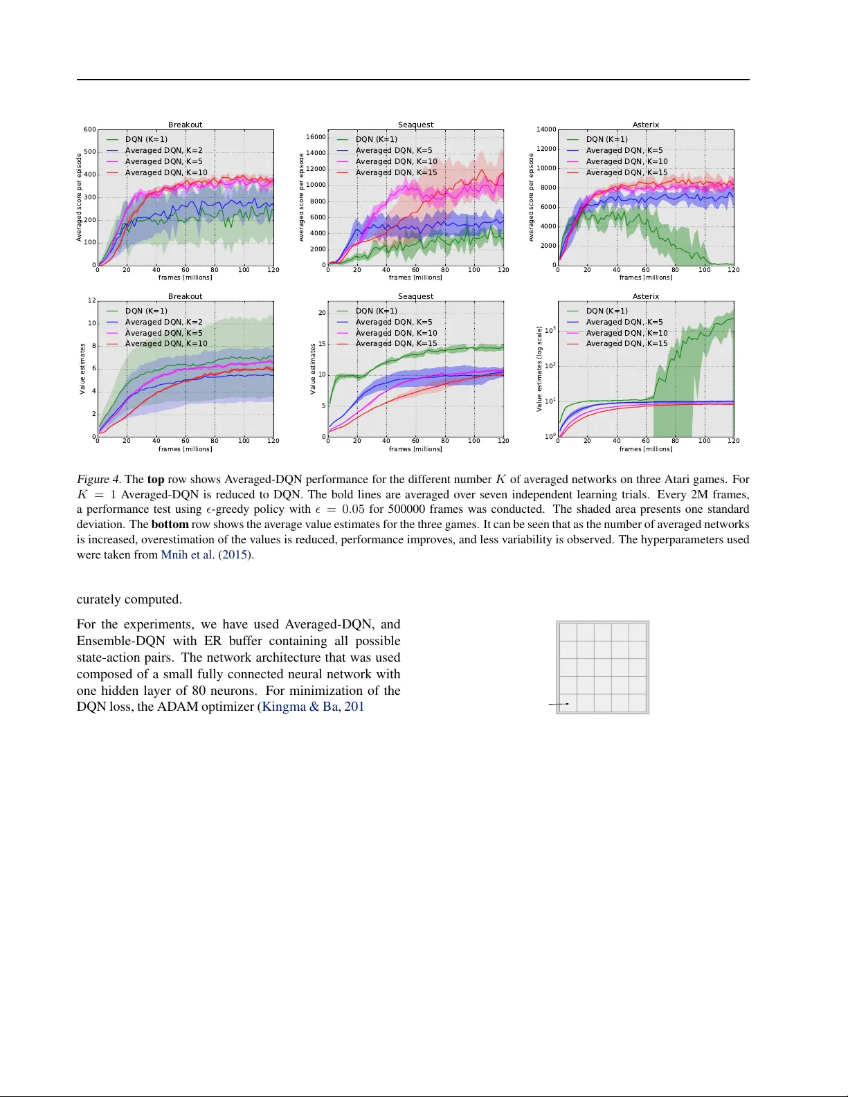
A veraged-DQN: V ariance Reduction and Stabilization f or Deep Reinf orcement Lear ning Oron Anschel 1 Nir Baram 1 Nahum Shimkin 1 Abstract Instability and variability of Deep Reinforcement Learning (DRL) algorithms tend to adversely af- fect their performance. A veraged-DQN is a sim- ple extension to the DQN algorithm, based on av eraging previously learned Q-v alues estimates, which leads to a more stable training procedure and improved performance by reducing approxi- mation error v ariance in the target v alues. T o un- derstand the effect of the algorithm, we examine the source of v alue function estimation errors and provide an analytical comparison within a sim- plified model. W e further present experiments on the Arcade Learning En vironment benchmark that demonstrate significantly improved stability and performance due to the proposed extension. 1. Introduction In Reinforcement Learning (RL) an agent seeks an opti- mal policy for a sequential decision making problem ( Sut- ton & Barto , 1998 ). It does so by learning which action is optimal for each en vironment state. Over the course of time, many algorithms have been introduced for solv- ing RL problems including Q-learning ( W atkins & Dayan , 1992 ), SARSA ( Rummery & Niranjan , 1994 ; Sutton & Barto , 1998 ), and policy gradient methods ( Sutton et al. , 1999 ). These methods are often analyzed in the setup of linear function approximation, where conv ergence is guar- anteed under mild assumptions ( Tsitsiklis , 1994 ; Jaakkola et al. , 1994 ; Tsitsiklis & V an Roy , 1997 ; Ev en-Dar & Man- sour , 2003 ). In practice, real-world problems usually in- volv e high-dimensional inputs forcing linear function ap- proximation methods to rely upon hand engineered features for problem-specific state representation. These problem- specific features diminish the agent fle xibility , and so the 1 Department of Electrical Engineering, Haifa 32000, Israel. Correspondence to: Oron Anschel < oronanschel@campus.technion.ac.il > , Nir Baram < nirb@campus.technion.ac.il > , Nahum Shimkin < shimkin@ee.technion.ac.il > . need of an expres siv e and fle xible non-linear function ap- proximation emerges. Except for fe w successful attempts (e.g., TD-gammon, T esauro ( 1995 )), the combination of non-linear function approximation and RL was considered unstable and w as shown to div erge e ven in simple domains ( Boyan & Moore , 1995 ). The recent Deep Q-Network (DQN) algorithm ( Mnih et al. , 2013 ), was the first to successfully combine a power - ful non-linear function approximation technique known as Deep Neural Network (DNN) ( LeCun et al. , 1998 ; Krizhevsk y et al. , 2012 ) together with the Q-learning al- gorithm. DQN presented a remarkably flexible and stable algorithm, showing success in the majority of games within the Arcade Learning En vironment (ALE) ( Bellemare et al. , 2013 ). DQN increased the training stability by breaking the RL problem into sequential supervised learning tasks. T o do so, DQN introduces the concept of a target network and uses an Experience Replay buf fer (ER) ( Lin , 1993 ). Follo wing the DQN work, additional modifications and ex- tensions to the basic algorithm further increased training stability . Schaul et al. ( 2015 ) suggested sophisticated ER sampling strategy . Sev eral works extended standard RL exploration techniques to deal with high-dimensional input ( Bellemare et al. , 2016 ; T ang et al. , 2016 ; Osband et al. , 2016 ). Mnih et al. ( 2016 ) showed that sampling from ER could be replaced with asynchronous updates from parallel en vironments (which enables the use of on-policy meth- ods). W ang et al. ( 2015 ) suggested a network architecture base on the advantage function decomposition ( Baird III , 1993 ). In this work we address issues that arise from the combi- nation of Q-learning and function approximation. Thrun & Schwartz ( 1993 ) were first to in vestigate one of these issues which they hav e termed as the over estimation phenomena . The max operator in Q-learning can lead to overestimation of state-action values in the presence of noise. V an Hasselt et al. ( 2015 ) suggest the Double-DQN that uses the Double Q-learning estimator ( V an Hasselt , 2010 ) method as a solu- tion to the problem. Additionally , V an Hasselt et al. ( 2015 ) showed that Q-learning overestimation do occur in practice (at least in the ALE). A veraged-DQN: V ariance Reduction and Stabilization for Deep Reinfor cement Learning This work suggests a dif ferent solution to the overestima- tion phenomena, named A veraged-DQN (Section 3 ), based on av eraging previously learned Q-values estimates. The av eraging reduces the target approximation error v ariance (Sections 4 and 5 ) which leads to stability and improv ed results. Additionally , we provide experimental results on selected games of the Arcade Learning En vironment. W e summarize the main contributions of this paper as fol- lows: • A novel e xtension to the DQN algorithm which stabi- lizes training, and impro ves the attained performance, by av eraging ov er previously learned Q-v alues. • V ariance analysis that explains some of the DQN problems, and how the proposed extension addresses them. • Experiments with several ALE games demonstrating the fa vorable ef fect of the proposed scheme. 2. Background In this section we elaborate on relev ant RL background, and specifically on the Q-learning algorithm. 2.1. Reinforcement Learning W e consider the usual RL learning framework ( Sutton & Barto , 1998 ). An agent is faced with a sequential deci- sion making problem, where interaction with the environ- ment takes place at discrete time steps ( t = 0 , 1 , . . . ). At time t the agent observes state s t ∈ S , selects an action a t ∈ A , which results in a scalar reward r t ∈ R , and a transition to a next state s t +1 ∈ S . W e consider infinite horizon problems with a discounted cumulati ve re ward ob- jectiv e R t = P ∞ t 0 = t γ t 0 − t r t 0 , where γ ∈ [0 , 1] is the dis- count factor . The goal of the agent is to find an optimal policy π : S → A that maximize its expected discounted cumulativ e re ward. V alue-based methods for solving RL problems encode poli- cies through the use of value functions, which denote the expected discounted cumulative rew ard from a giv en state s , following a polic y π . Specifically we are interested in state-action value functions: Q π ( s, a ) = E π " ∞ X t =0 γ t r t | s 0 = s, a 0 = a # . The optimal v alue function is denoted as Q ∗ ( s, a ) = max π Q π ( s, a ) , and an optimal policy π ∗ can be easily de- riv ed by π ∗ ( s ) ∈ argmax a Q ∗ ( s, a ) . 2.2. Q-learning One of the most popular RL algorithms is the Q-learning algorithm ( W atkins & Dayan , 1992 ). This algorithm is based on a simple value iteration update ( Bellman , 1957 ), directly estimating the optimal value function Q ∗ . T ab ular Q-learning assumes a table that contains old action-v alue function estimates and preform updates using the follo w- ing update rule: Q ( s, a ) ← Q ( s, a ) + α ( r + γ max a 0 Q ( s 0 , a 0 ) − Q ( s, a )) , (1) where s 0 is the resulting state after applying action a in the state s , r is the immediate reward observed for action a at state s , γ is the discount factor , and α is a learning rate. When the number of states is large, maintaining a look- up table with all possible state-action pairs values in mem- ory is impractical. A common solution to this issue is to use function approximation parametrized by θ , such that Q ( s, a ) ≈ Q ( s, a ; θ ) . 2.3. Deep Q Networks (DQN) W e present in Algorithm 1 a slightly different formulation of the DQN algorithm ( Mnih et al. , 2013 ). In iteration i the DQN algorithm solv es a supervised learning problem to approximate the action-value function Q ( s, a ; θ ) (line 6). This is an extension of implementing ( 1 ) in its function ap- proximation form ( Riedmiller , 2005 ). Algorithm 1 DQN 1: Initialize Q ( s, a ; θ ) with random weights θ 0 2: Initialize Experience Replay (ER) buf fer B 3: Initialize exploration procedure Explor e( · ) 4: for i = 1 , 2 , . . . , N do 5: y i s,a = E B [ r + γ max a 0 Q ( s 0 , a 0 ; θ i − 1 ) | s, a ] 6: θ i ≈ argmin θ E B  ( y i s,a − Q ( s, a ; θ )) 2  7: Explor e( · ) , update B 8: end f or output Q DQN ( s, a ; θ N ) The target values y i s,a (line 5) are constructed using a desig- nated targ et-network Q ( s, a ; θ i − 1 ) (using the previous iter- ation parameters θ i − 1 ), where the e xpectation ( E B ) is taken w .r .t. the sample distribution of experience transitions in the ER buf fer ( s, a, r , s 0 ) ∼ B . The DQN loss (line 6) is mini- mized using a Stochastic Gradient Descent (SGD) variant, sampling mini-batches from the ER buf fer . Additionally , DQN requires an exploration procedure (which we denote as Explor e( · ) ) to interact with the en vironment (e.g., an  - greedy exploration procedure). The number of ne w e xperi- ence transitions ( s, a, r, s 0 ) added by exploration to the ER A veraged-DQN: V ariance Reduction and Stabilization for Deep Reinfor cement Learning buf fer in each iteration is small, relativ ely to the size of the ER buf fer . Thereby , θ i − 1 can be used as a good initializa- tion for θ in iteration i . Note that in the original implementation ( Mnih et al. , 2013 ; 2015 ), transitions are added to the ER buf fer simultane- ously with the minimization of the DQN loss (line 6). Us- ing the hyperparameters employed by Mnih et al. ( 2013 ; 2015 ) (detailed for completeness in Appendix D ), 1% of the experience transitions in ER buf fer are replaced be- tween target network parameter updates, and 8% are sam- pled for minimization. 3. A veraged DQN The A veraged-DQN algorithm (Algorithm 2 ) is an exten- sion of the DQN algorithm. A veraged-DQN uses the K previously learned Q-v alues estimates to produce the cur- rent action-value estimate (line 5). The A veraged-DQN al- gorithm stabilizes the training process (see Figure 1 ), by reducing the variance of targ et appr oximation err or as we elaborate in Section 5 . The computational effort com- pared to DQN is, K -fold more forward passes through a Q-network while minimizing the DQN loss (line 7). The number of back-propagation updates (which is the most de- manding computational element), remains the same as in DQN. The output of the algorithm is the a verage over the last K previously learned Q-networks. 0 20 40 60 80 100 120 frames [millions] 0 100 200 300 400 500 Averaged score per episode Breakout DQN Averaged DQN, K=10 Figure 1. DQN and A veraged-DQN performance in the Atari game of B R E A K O U T . The bold lines are av erages o ver seven in- dependent learning trials. Every 1M frames, a performance test using  -greedy policy with  = 0 . 05 for 500000 frames was con- ducted. The shaded area presents one standard deviation. F or both DQN and A veraged-DQN the hyperparameters used were taken from Mnih et al. ( 2015 ). In Figures 1 and 2 we can see the performance of A veraged- Algorithm 2 A veraged DQN 1: Initialize Q ( s, a ; θ ) with random weights θ 0 2: Initialize Experience Replay (ER) buf fer B 3: Initialize exploration procedure Explor e ( · ) 4: for i = 1 , 2 , . . . , N do 5: Q A i − 1 ( s, a ) = 1 K P K k =1 Q ( s, a ; θ i − k ) 6: y i s,a = E B  r + γ max a 0 Q A i − 1 ( s 0 , a 0 ) | s, a  7: θ i ≈ argmin θ E B  ( y i s,a − Q ( s, a ; θ )) 2  8: Explor e( · ) , update B 9: end f or output Q A N ( s, a ) = 1 K P K − 1 k =0 Q ( s, a ; θ N − k ) DQN compared to DQN (and Double-DQN), further exper - imental results are giv en in Section 6 . W e note that recently-learned state-action v alue estimates are likely to be better than older ones, therefore we have also considered a recency-weighted average. In practice, a weighted a verage scheme did not improve performance and therefore is not presented here. 4. Overestimation and Appr oximation Errors Next, we discuss the various types of errors that arise due to the combination of Q-learning and function approximation in the DQN algorithm, and their effect on training stability . W e refer to DQN’ s performance in the B R E A K O U T game in Figure 1 . The source of the learning curve variance in DQN’ s performance is an occasional sudden drop in the av erage score that is usually recovered in the next ev alua- tion phase (for another illustration of the variance source see Appendix A ). Another phenomenon can be observ ed in Figure 2 , where DQN initially reaches a steady state (after 20 million frames), followed by a gradual deterioration in performance. For the rest of this section, we list the abov e mentioned er- rors, and discuss our hypothesis as to the relations between each error and the instability phenomena depicted in Fig- ures 1 and 2 . W e follow terminology from Thrun & Schwartz ( 1993 ), and define some additional rele vant quantities. Letting Q ( s, a ; θ i ) be the v alue function of DQN at iteration i , we denote ∆ i = Q ( s, a ; θ i ) − Q ∗ ( s, a ) and decompose it as follows: ∆ i = Q ( s, a ; θ i ) − Q ∗ ( s, a ) = Q ( s, a ; θ i ) − y i s,a | {z } T arg et Approximation Err or + y i s,a − ˆ y i s,a | {z } Over estimation Err or + ˆ y i s,a − Q ∗ ( s, a ) | {z } Optimality Differ ence . A veraged-DQN: V ariance Reduction and Stabilization for Deep Reinfor cement Learning 0 20 40 60 80 100 120 frames [millions] 0 2000 4000 6000 8000 10000 Averaged score per episode Asterix DQN Double - DQN Averaged DQN, K=10 20 40 60 80 100 120 frames [millions] 1 0 - 1 1 0 0 1 0 1 1 0 2 1 0 3 1 0 4 Value estimates (log scale) Asterix DQN Double - DQN Averaged DQN, K=10 Figure 2. DQN, Double-DQN, and A veraged-DQN performance (left), and average value estimates (right) in the Atari game of A S T E R I X . The bold lines are averages over se ven independent learning trials. The shaded area presents one standard deviation. Every 2M frames, a performance test using  -greedy policy with  = 0 . 05 for 500000 frames was conducted. The hyperparameters used were taken from Mnih et al. ( 2015 ). Here y i s,a is the DQN tar get , and ˆ y i s,a is the true tar get : y i s,a = E B h r + γ max a 0 Q ( s 0 , a 0 ; θ i − 1 ) | s, a i , ˆ y i s,a = E B h r + γ max a 0 ( y i − 1 s 0 ,a 0 ) | s, a i . Let us denote by Z i s,a the target approximation error, and by R i s,a the ov erestimation error, namely Z i s,a = Q ( s, a ; θ i ) − y i s,a , R i s,a = y i s,a − ˆ y i s,a . The optimality dif ference can be seen as the error of a stan- dard tabular Q-learning, here we address the other errors. W e next discuss each error in turn. 4.1. T arget Appr oximation Error (T AE) The T AE ( Z i s,a ), is the error in the learned Q ( s, a ; θ i ) rela- tiv e to y i s,a , which is determined after minimizing the DQN loss (Algorithm 1 line 6, Algorithm 2 line 7). The T AE is a result of sev eral factors: Firstly , the sub-optimality of θ i due to inexact minimization. Secondly , the limited repre- sentation power of a neural net (model error). Lastly , the generalization error for unseen state-action pairs due to the finite size of the ER buf fer . The T AE can cause a de viations from a policy to a worse one. For example, such deviation to a sub-optimal policy occurs in case y i s,a = ˆ y i s,a = Q ∗ ( s, a ) and, argmax a [ Q ( s, a ; θ i )] 6 = argmax a [ Q ( s, a ; θ i ) − Z i s,a ] = argmax a [ y i s,a ] . W e hypothesize that the variability in DQN’ s performance in Figure 1 , that was discussed at the start of this section, is related to de viating from a steady-state policy induced by the T AE. 4.2. Overestimation Error The Q-learning overestimation phenomena were first in ves- tigated by Thrun & Schwartz ( 1993 ). In their work, Thrun and Schw artz considered the T AE Z i s,a as a random v ari- able uniformly distrib uted in the interval [ − ,  ] . Due to the max operator in the DQN target y i s,a , the expected over - estimation errors E z [ R i s,a ] are upper bounded by γ  n − 1 n +1 (where n is the number of applicable actions in state s ). The intuition for this upper bound is that in the worst case, all Q values are equal, and we get equality to the upper bound: E z [ R i s,a ] = γ E z [max a 0 [ Z i − 1 s 0 ,a 0 ]] = γ  n − 1 n + 1 . The overestimation error is different in its nature from the T AE since it presents a positive bias that can cause asymp- totically sub-optimal policies, as was shown by Thrun & Schwartz ( 1993 ), and later by V an Hasselt et al. ( 2015 ) in the ALE en vironment. Note that a uniform bias in the action-value function will not cause a change in the induced policy . Unfortunately , the overestimation bias is unev en and is bigger in states where the Q-values are similar for the different actions, or in states which are the start of a long trajectory (as we discuss in Section 5 on accumulation of T AE variance). Follo wing from the abo ve mentioned o verestimation upper bound, the magnitude of the bias is controlled by the vari- ance of the T AE. A veraged-DQN: V ariance Reduction and Stabilization for Deep Reinfor cement Learning The Double Q-learning and its DQN implementation (Double-DQN) ( V an Hasselt et al. , 2015 ; V an Hasselt , 2010 ) is one possible approach to tackle the o verestimation problem, which replaces the positiv e bias with a neg ativ e one. Another possible remedy to the adverse effects of this error is to directly reduce the variance of the T AE, as in our proposed scheme (Section 5 ). In Figure 2 we repeated the experiment presented in V an Hasselt et al. ( 2015 ) (along with the application of A veraged-DQN). This experiment is discussed in V an Has- selt et al. ( 2015 ) as an example of ov erestimation that leads to asymptotically sub-optimal policies. Since A veraged- DQN reduces the T AE v ariance, this experiment supports an hypothesis that the main cause for overestimation in DQN is the T AE variance. 5. T AE V ariance Reduction T o analyse the T AE variance we first must assume a statis- tical model on the T AE, and we do so in a similar way to Thrun & Schwartz ( 1993 ). Suppose that the T AE Z i s,a is a random process such that E [ Z i s,a ] = 0 , V ar [ Z i s,a ] = σ 2 s , and for i 6 = j : Cov [ Z i s,a , Z j s 0 ,a 0 ] = 0 . Furthermore, to fo- cus only on the T AE we eliminate the overestimation error by considering a fixed policy for updating the target values. Also, we can con veniently consider a zero rew ard r = 0 ev erywhere since it has no ef fect on variance calculations. Denote by Q i , Q ( s ; θ i ) s ∈ S the vector of value estimates in iteration i (where the fixed action a is suppressed), and by Z i the vector of corresponding T AEs. For A veraged- DQN we get: Q i = Z i + γ P 1 K K X k =1 Q i − k , where P ∈ R S × S + is the transition probabilities matrix for the gi ven policy . Assuming stationarity of Q i , its cov ari- ance can be obtained using standard techniques (e.g., as a solution of a linear equations system). Howe ver , to obtain an explicit comparison, we further specialize the model to an M -state unidirectional MDP as in Figure 3 s 0 s 1 · · · s M − 2 s M − 1 a a a a Figure 3. M states unidirectional MDP , The process starts at state s 0 , then in each time step moves to the right, until the terminal state s M − 1 is reached. A zero rew ard is obtained in any state. 5.1. DQN V ariance W e assume the statistical model mentioned at the start of this section. Consider a unidirectional Markov Decision Process (MDP) as in Figure 3 , where the agent starts at state s 0 , state s M − 1 is a terminal state, and the re ward in any state is equal to zero. Employing DQN on this MDP model, we get that for i > M : Q DQN ( s 0 , a ; θ i ) = Z i s 0 ,a + y i s 0 ,a = Z i s 0 ,a + γ Q ( s 1 , a ; θ i − 1 ) = Z i s 0 ,a + γ [ Z i − 1 s 1 ,a + y i − 1 s 1 ,a ] = · · · = = Z i s 0 ,a + γ Z i − 1 s 1 ,a + · · · + γ ( M − 1) Z i − ( M − 1) s M − 1 ,a , where in the last equality we have used the fact y j M − 1 ,a = 0 for all j (terminal state). Therefore, V ar [ Q DQN ( s 0 , a ; θ i )] = M − 1 X m =0 γ 2 m σ 2 s m . The abov e example gives intuition about the behavior of the T AE v ariance in DQN. The T AE is accumulated ov er the past DQN iterations on the updates trajectory . Accu- mulation of T AE errors results in bigger variance with its associated adverse ef fect, as was discussed in Section 4 . Algorithm 3 Ensemble DQN 1: Initialize K Q-networks Q ( s, a ; θ k ) with random weights θ k 0 for k ∈ { 1 , . . . , K } 2: Initialize Experience Replay (ER) buf fer B 3: Initialize exploration procedure Explor e( · ) 4: for i = 1 , 2 , . . . , N do 5: Q E i − 1 ( s, a ) = 1 K P K k =1 Q ( s, a ; θ k i − 1 ) 6: y i s,a = E B  r + γ max a 0 Q E i − 1 ( s 0 , a 0 )) | s, a  7: for k = 1 , 2 , . . . , K do 8: θ k i ≈ argmin θ E B  ( y i s,a − Q ( s, a ; θ )) 2  9: end for 10: Explor e( · ) , update B 11: end f or output Q E N ( s, a ) = 1 K P K k =1 Q ( s, a ; θ k i ) 5.2. Ensemble DQN V ariance W e consider two approaches for T AE variance reduction. The first one is the A veraged-DQN and the second we term Ensemble-DQN . W e start with Ensemble-DQN which is a straightforward way to obtain a 1 /K variance reduction, A veraged-DQN: V ariance Reduction and Stabilization for Deep Reinfor cement Learning with a computational ef fort of K -fold learning problems, compared to DQN. Ensemble-DQN (Algorithm 3 ) solves K DQN losses in parallel, then av erages over the resulted Q-values estimates. For Ensemble-DQN on the unidirectional MDP in Figure 3 , we get for i > M : Q E i ( s 0 , a ) = M − 1 X m =0 γ m 1 K K X k =1 Z k,i − m s m ,a , V ar [ Q E i ( s 0 , a )] = M − 1 X m =0 1 K γ 2 m σ 2 s m = 1 K V ar [ Q DQN ( s 0 , a ; θ i )] , where for k 6 = k 0 : Z k,i s,a and Z k 0 ,j s 0 ,a 0 are two uncorrelated T AEs. The calculations of Q E ( s 0 , a ) are detailed in Ap- pendix B . 5.3. A veraged DQN V ariance W e continue with A veraged-DQN, and calculate the v ari- ance in state s 0 for the unidirectional MDP in Figure 3 . W e get that for i > K M : V ar [ Q A i ( s 0 , a )] = M − 1 X m =0 D K,m γ 2 m σ 2 s m , where D K,m = 1 N P N − 1 n =0 | U n /K | 2( m +1) , with U = ( U n ) N − 1 n =0 denoting a Discrete Fourier T ransform (DFT) of a rectangle pulse, and | U n /K | ≤ 1 . The calculations of Q A ( s 0 , a ) and D K,m are more inv olved and are detailed in Appendix C . Furthermore, for K > 1 , m > 0 we have that D K,m < 1 /K (Appendix C ) and therefore the following holds V ar [ Q A i ( s 0 , a )] < V ar [ Q E i ( s 0 , a )] = 1 K V ar [ Q DQN ( s 0 , a ; θ i )] , meaning that A veraged-DQN is theoretically more efficient in T AE variance reduction than Ensemble-DQN, and at least K times better than DQN. The intuition here is that A veraged-DQN averages ov er T AEs averages, which are the value estimates of the ne xt states. 6. Experiments The experiments were designed to address the following questions: • How does the number K of averaged target networks affect the error in value estimates, and in particular the ov erestimation error . • How does the averaging affect the learned polices quality . T o that end, we ran A veraged-DQN and DQN on the ALE benchmark. Additionally , we ran A veraged-DQN, Ensemble-DQN, and DQN on a Gridworld toy problem where the optimal v alue function can be computed exactly . 6.1. Arcade Learning Envir onment (ALE) T o ev aluate A veraged-DQN, we adopt the typical RL methodology where agent performance is measured at the end of training. W e refer the reader to Liang et al. ( 2016 ) for further discussion about DQN ev aluation methods on the ALE benchmark. The hyperparameters used were taken from Mnih et al. ( 2015 ), and are presented for complete- ness in Appendix D . DQN code was taken from McGill Univ ersity RLLAB, and is av ailable online 1 (together with A veraged-DQN implementation). W e ha ve ev aluated the A veraged-DQN algorithm on three Atari games from the Arcade Learning En vironment ( Bellemare et al. , 2013 ). The game of B R E A K O U T was selected due to its popularity and the relative ease of the DQN to reach a steady state policy . In contrast, the game of S E AQ U E S T was selected due to its relative complexity , and the significant improv ement in performance obtained by other DQN variants (e.g., Schaul et al. ( 2015 ); W ang et al. ( 2015 )). Finally , the game of A S T E R I X was presented in V an Hasselt et al. ( 2015 ) as an example to overestimation in DQN that leads to div ergence. As can be seen in Figure 4 and in T able 1 for all three games, increasing the number of averaged networks in A veraged-DQN results in lower average values estimates, better-preforming policies, and less v ariability between the runs of independent learning trials. For the game of A S - T E R I X , we see similarly to V an Hasselt et al. ( 2015 ) that the div ergence of DQN can be pre vented by av eraging. Overall, the results suggest that in practice A veraged-DQN reduces the T AE v ariance, which leads to smaller ov eres- timation, stabilized learning curves and significantly im- prov ed performance. 6.2. Gridworld The Gridw orld problem (Figure 5 ) is a common RL bench- mark (e.g., Boyan & Moore ( 1995 )). As opposed to the ALE, Gridworld has a smaller state space that allo ws the ER buf fer to contain all possible state-action pairs. Addi- tionally , it allows the optimal value function Q ∗ to be ac- 1 McGill Univ ersity RLLAB DQN Atari code: https: //bitbucket.org/rllabmcgill/atari_release . A veraged-DQN code https://bitbucket.org/ oronanschel/atari_release_averaged_dqn A veraged-DQN: V ariance Reduction and Stabilization for Deep Reinfor cement Learning 0 20 40 60 80 100 120 frames [millions] 0 100 200 300 400 500 600 Averaged score per episode Breakout DQN (K=1) Averaged DQN, K=2 Averaged DQN, K=5 Averaged DQN, K=10 0 20 40 60 80 100 120 frames [millions] 0 2000 4000 6000 8000 10000 12000 14000 16000 Averaged score per episode Seaquest DQN (K=1) Averaged DQN, K=5 Averaged DQN, K=10 Averaged DQN, K=15 0 20 40 60 80 100 120 frames [millions] 0 2000 4000 6000 8000 10000 12000 14000 Averaged score per episode Asterix DQN (K=1) Averaged DQN, K=5 Averaged DQN, K=10 Averaged DQN, K=15 0 20 40 60 80 100 120 frames [millions] 0 2 4 6 8 10 12 Value estimates Breakout DQN (K=1) Averaged DQN, K=2 Averaged DQN, K=5 Averaged DQN, K=10 0 20 40 60 80 100 120 frames [millions] 0 5 10 15 20 Value estimates Seaquest DQN (K=1) Averaged DQN, K=5 Averaged DQN, K=10 Averaged DQN, K=15 0 20 40 60 80 100 120 frames [millions] 1 0 0 1 0 1 1 0 2 1 0 3 Value estimates (log scale) Asterix DQN (K=1) Averaged DQN, K=5 Averaged DQN, K=10 Averaged DQN, K=15 Figure 4. The top row shows A veraged-DQN performance for the different number K of av eraged networks on three Atari games. For K = 1 A veraged-DQN is reduced to DQN. The bold lines are averaged over seven independent learning trials. Every 2M frames, a performance test using  -greedy policy with  = 0 . 05 for 500000 frames was conducted. The shaded area presents one standard deviation. The bottom row shows the a verage value estimates for the three games. It can be seen that as the number of averaged networks is increased, overestimation of the v alues is reduced, performance improv es, and less variability is observed. The hyperparameters used were taken from Mnih et al. ( 2015 ). curately computed. For the experiments, we have used A veraged-DQN, and Ensemble-DQN with ER buf fer containing all possible state-action pairs. The network architecture that was used composed of a small fully connected neural network with one hidden layer of 80 neurons. For minimization of the DQN loss, the ADAM optimizer ( Kingma & Ba , 2014 ) was used on 100 mini-batches of 32 samples per tar get network parameters update in the first experiment, and 300 mini- batches in the second. 6 . 2 . 1 . E N V I R O N M E N T S E T U P In this experiment on the problem of Gridworld (Figure 5 ), the state space contains pairs of points from a 2D dis- crete grid ( S = { ( x, y ) } x,y ∈ 1 ,..., 20 ). The algorithm inter- acts with the environment through raw pixel features with a one-hot feature map φ ( s t ) := ( 1 { s t = ( x, y ) } ) x,y ∈ 1 ,..., 20 . There are four actions corresponding to steps in each com- pass direction, a reward of r = +1 in state s t = (20 , 20) , and r = 0 otherwise. W e consider the discounted return problem with a discount factor of γ = 0 . 9 . +1 start Gridworld Figure 5. Gridworld problem. The agent starts at the left-bottom of the grid. In the upper-right corner , a reward of +1 is obtained. 6 . 2 . 2 . O V E R E S T I M AT I O N In Figure 6 it can be seen that increasing the number K of av eraged target networks leads to reduced ov erestimation ev entually . Also, more averaged target networks seem to reduces the overshoot of the values, and leads to smoother and less inconsistent con ver gence. 6 . 2 . 3 . A V E R AG E D V E R S U S E N S E M B L E D Q N In Figure 7 , it can be seen that as was predicted by the analysis in Section 5 , Ensemble-DQN is also inferior to A veraged-DQN regarding variance reduction, and as a con- A veraged-DQN: V ariance Reduction and Stabilization for Deep Reinfor cement Learning T able 1. The columns present the av erage performance of DQN and A veraged-DQN after 120M frames, using  -greedy policy with  = 0 . 05 for 500000 frames. The standard variation represents the v ariability over sev en independent trials. A verage performance improv ed with the number of averaged netw orks. Human and random performance were taken from Mnih et al. ( 2015 ). G A M E D Q N A V E R A G E D - D Q N A V E R A G E D - D Q N A V E R A G E D - D Q N H U M A N R A N D O M A V G . ( S T D . D E V . ) ( K = 5 ) ( K = 1 0 ) ( K = 1 5 ) B R E A K O U T 2 4 5 . 1 ( 1 2 4 . 5 ) 3 8 1 . 5 ( 2 0 . 2 ) 3 8 1 . 8 ( 2 4 . 2 ) - - 3 1 . 8 1 . 7 S E AQ U E S T 3 7 7 5 . 2 ( 1 5 7 5 . 6 ) 5 7 4 0 . 2 ( 6 6 4 . 7 9 ) 9 9 6 1 . 7 ( 1 9 4 6 . 9 ) 1 0 4 7 5 . 1 ( 2 9 2 6 . 6 ) 2 0 1 8 2 . 0 6 8 . 4 A S T E R I X 1 9 5 . 6 ( 8 0 . 4 ) 6 9 6 0 . 0 ( 9 9 9 . 2 ) 8 0 0 8 . 3 ( 2 4 3 . 6 ) 8 3 6 4 . 9 ( 6 1 8 . 6 ) 85 0 3 . 0 2 1 0 . 0 200 400 600 800 1000 Iter ations 1 . 90 1 . 92 1 . 94 1 . 96 1 . 98 2 . 00 2 . 02 2 . 04 2 . 06 A v er age predicted v alue A B C D Gr idw or ld E s [ max a Q ∗ ( s, a )] DQN (K=1) A v er aged DQN, K=5 A v er aged DQN, K=10 A v er aged DQN, K=20 Figure 6. A veraged-DQN a verage predicted value in Gridw orld. Increasing the number K of averaged tar get networks leads to a faster con vergence with less overestimation (positi ve-bias). The bold lines are a verages over 40 independent learning trials, and the shaded area presents one standard deviation. In the figure, A,B,C,D present DQN, and A veraged-DQN for K=5,10,20 av er- age ov erestimation. sequence far more overestimates the v alues. W e note that Ensemble-DQN was not implemented for the ALE exper- iments due to its demanding computational effort, and the empirical e vidence that was already obtained in this simple Gridworld domain. 7. Discussion and Future Directions In this work, we have presented the A veraged-DQN algo- rithm, an e xtension to DQN that stabilizes training, and im- prov es performance by efficient T AE variance reduction. W e hav e shown both in theory and in practice that the pro- posed scheme is superior in T AE variance reduction, com- pared to a straightforward but computationally demanding approach such as Ensemble-DQN (Algorithm 3 ). W e have demonstrated in sev eral games of Atari that increasing the number K of av eraged target networks leads to better poli- 0 200 400 600 800 1000 Iter ations 1 . 90 1 . 92 1 . 94 1 . 96 1 . 98 2 . 00 2 . 02 2 . 04 A v er age predicted v alue Gr idw or ld E s [ max a Q ∗ ( s, a )] DQN (K=1) Ensemb le DQN, K=20 A v er aged DQN, K=20 Figure 7. A veraged-DQN and Ensemble-DQN predicted value in Gridworld. A veraging of past learned value is more beneficial than learning in parallel. The bold lines are averages ov er 20 independent learning trials, where the shaded area presents one standard deviation. cies while reducing overestimation. A veraged-DQN is a simple extension that can be easily integrated with other DQN variants such as Schaul et al. ( 2015 ); V an Hasselt et al. ( 2015 ); W ang et al. ( 2015 ); Bellemare et al. ( 2016 ); He et al. ( 2016 ). Indeed, it would be of interest to study the added value of averaging when combined with these variants. Also, since A veraged-DQN has v ariance reduc- tion effect on the learning curve, a more systematic com- parison between the different variants can be facilitated as discussed in ( Liang et al. , 2016 ). In future work, we may dynamically learn when and how many networks to a verage for best results. One simple sug- gestion may be to correlate the number of networks with the state TD-error , similarly to Schaul et al. ( 2015 ). Finally , incorporating averaging techniques similar to A veraged- DQN within on-policy methods such as SARSA and Actor- Critic methods ( Mnih et al. , 2016 ) can further stabilize these algorithms. A veraged-DQN: V ariance Reduction and Stabilization for Deep Reinfor cement Learning References Baird III, Leemon C. Advantage updating. T echnical re- port, DTIC Document, 1993. Bellemare, M. G., Naddaf, Y ., V eness, J., and Bowling, M. The arcade learning en vironment: An ev aluation plat- form for general agents. Journal of Artificial Intelligence Resear ch , 47:253–279, 2013. Bellemare, Marc G, Sriniv asan, Sriram, Ostrovski, Georg, Schaul, T om, Saxton, David, and Munos, Remi. Uni- fying count-based exploration and intrinsic motiv ation. arXiv pr eprint arXiv:1606.01868 , 2016. Bellman, Richard. A Mark ovian decision process. Indiana Univ . Math. J . , 6:679–684, 1957. Boyan, Justin and Moore, Andrew W . Generalization in reinforcement learning: Safely approximating the value function. Advances in neural information processing systems , pp. 369–376, 1995. Even-Dar , Eyal and Mansour , Y ishay . Learning rates for q-learning. J ournal of Machine Learning Researc h , 5 (Dec):1–25, 2003. He, Frank S., Y ang Liu, Alexander G. Schwing, and Peng, Jian. Learning to play in a day: Faster deep reinforce- ment learning by optimality tightening. arXiv preprint arXiv:1611.01606 , 2016. Jaakkola, T ommi, Jordan, Michael I, and Singh, Satinder P . On the con ver gence of stochastic iterativ e dynamic pro- gramming algorithms. Neural Computation , 6(6):1185– 1201, 1994. Kingma, Diederik P . and Ba, Jimmy . Adam: A method for stochastic optimization. arXiv preprint arXiv: 1412.6980 , 2014. Krizhevsk y , Alex, Sutsk ev er , Ilya, and Hinton, Geof frey E. Imagenet classification with deep con volutional neural networks. In Advances in NIPS , pp. 1097–1105, 2012. LeCun, Y ann, Bottou, L ´ eon, Bengio, Y oshua, and Haffner , Patrick. Gradient-based learning applied to document recognition. Pr oceedings of the IEEE , 86(11):2278– 2324, 1998. Liang, Y itao, Machado, Marlos C, T alvitie, Erik, and Bowl- ing, Michael. State of the art control of Atari games using shallow reinforcement learning. In Proceedings of the 2016 International Confer ence on Autonomous Agents & Multiag ent Systems , pp. 485–493, 2016. Lin, Long-Ji. Reinforcement learning for robots using neu- ral networks. T echnical report, DTIC Document, 1993. Mnih, V olodymyr, Ka vukcuoglu, Koray , Silver , David, Grav es, Alex, Antonoglou, Ioannis, W ierstra, Daan, and Riedmiller , Martin. Playing Atari with deep reinforce- ment learning. arXiv preprint , 2013. Mnih, V olodymyr, Ka vukcuoglu, Koray , Silver , David, Rusu, Andrei A, V eness, Joel, Bellemare, Marc G, Grav es, Alex, Riedmiller , Martin, Fidjeland, Andreas K, Ostrovski, Georg, et al. Human-le vel control through deep reinforcement learning. Natur e , 518(7540):529– 533, 2015. Mnih, V olodymyr , Badia, Adria Puigdomenech, Mirza, Mehdi, Graves, Alex, Lillicrap, T imothy P , Harley , Tim, Silver , David, and Kavukcuoglu, Koray . Asynchronous methods for deep reinforcement learning. arXiv pr eprint arXiv:1602.01783 , 2016. Osband, Ian, Blundell, Charles, Pritzel, Alexander , and V an Roy , Benjamin. Deep exploration via bootstrapped DQN. arXiv preprint , 2016. Riedmiller , Martin. Neural fitted Q iteration–first experi- ences with a data ef ficient neural reinforcement learning method. In Eur opean Confer ence on Machine Learning , pp. 317–328. Springer , 2005. Rummery , Gavin A and Niranjan, Mahesan. On-line Q- learning using connectionist systems . Univ ersity of Cambridge, Department of Engineering, 1994. Schaul, T om, Quan, John, Antonoglou, Ioannis, and Sil- ver , David. Prioritized e xperience replay . arXiv pr eprint arXiv:1511.05952 , 2015. Sutton, Richard S and Barto, Andrew G. Reinforcement Learning: An Intr oduction . MIT Press Cambridge, 1998. Sutton, Richard S, McAllester , David A, Singh, Satinder P , and Mansour , Y ishay . Policy gradient methods for re- inforcement learning with function approximation. In NIPS , volume 99, pp. 1057–1063, 1999. T ang, Haoran, Rein Houthooft, Davis Foote, Adam Stooke, Xi Chen, Y an Duan, John Schulman, and Filip De T urck, Pieter Abbeel. #exploration: A study of count-based ex- ploration for deep reinforcement learning. arXiv preprint arXiv:1611.04717 , 2016. T esauro, Gerald. T emporal difference learning and td- gammon. Communications of the ACM , 38(3):58–68, 1995. Thrun, Sebastian and Schwartz, Anton. Issues in using function approximation for reinforcement learning. In Pr oceedings of the 1993 Connectionist Models Summer School Hillsdale, NJ . Lawrence Erlbaum , 1993. A veraged-DQN: V ariance Reduction and Stabilization for Deep Reinfor cement Learning Tsitsiklis, John N. Asynchronous stochastic approxima- tion and q-learning. Machine Learning , 16(3):185–202, 1994. Tsitsiklis, John N and V an Roy , Benjamin. An analysis of temporal-difference learning with function approxi- mation. IEEE transactions on automatic contr ol , 42(5): 674–690, 1997. V an Hasselt, Hado. Double Q-learning. In Lafferty , J. D., W illiams, C. K. I., Shawe-T aylor , J., Zemel, R. S., and Culotta, A. (eds.), Advances in Neural Information Pr o- cessing Systems 23 , pp. 2613–2621. 2010. V an Hasselt, Hado, Guez, Arthur , and Silver , David. Deep reinforcement learning with double Q-learning. arXiv pr eprint arXiv: 1509.06461 , 2015. W ang, Ziyu, de Freitas, Nando, and Lanctot, Marc. Dueling network architectures for deep reinforcement learning. arXiv pr eprint arXiv: 1511.06581 , 2015. W atkins, Christopher JCH and Dayan, Peter . Q-learning. Machine Learning , 8(3-4):279–292, 1992. A veraged-DQN: V ariance Reduction and Stabilization for Deep Reinfor cement Learning A. DQN V ariance Source Example Figure 8 presents a single learning trial of DQN compared to A veraged-DQN, which emphasizes that the source of variability in DQN between learning trials is due to occa- sions drops in av erage score within the learning trial. As suggested in Section 4 , this effect can be related to the T AE causing to a deviation from the steady state polic y . B. Ensemble DQN T AE V ariance Calculation in a unidirectional MDP (Section 5.2 ) Recall that E [ Z k,i s,a ] = 0 , V ar [ Z k,i s,a ] = σ 2 s , for all i 6 = j : Cov [ Z k,i s,a , Z k 0 ,j s 0 ,a ] = 0 , and for all k 6 = k 0 : Cov [ Z k,i s,a , Z k 0 ,j s 0 ,a ] = 0 . Following the Ensemble-DQN up- date equations in Algorithm 3 : Q E i ( s 0 , a ) = = 1 K K X k =1 Q ( s 0 , a ; θ k i ) = 1 K K X k =1 [ Z k,i s 0 ,a + y i s 0 ,a ] = 1 K K X k =1 [ Z k,i s 0 ,a ] + y i s 0 ,a = 1 K K X k =1 [ Z k,i s 0 ,a ] + γ Q E i − 1 ( s 1 , a ) = 1 K K X k =1 [ Z k,i s 0 ,a ] + γ K K X k =1 [ Z k,i − 1 s 1 ,a ] + γ y i − 1 s 2 ,a . By iterati vely expanding y i − 1 s 2 ,a as abov e, and noting that y j s M − 1 ,a = 0 for all times (terminal state), we obtain, Q E i ( s 0 , a ) = M − 1 X m =0 γ m 1 K K X k =1 Z k,i − m s m ,a . Since the T AEs are uncorrelated by assumption, we get V ar [ Q E i ( s 0 , a )] = M − 1 X m =0 1 K γ 2 m σ 2 s m . C. A veraged DQN T AE V ariance Calculation in a unidirectional MDP (Section 5.3 ) Recall that E [ Z i s,a ] = 0 , V ar [ Z i s,a ] = σ 2 s , and for i 6 = j : Cov [ Z i s,a , Z j s 0 ,a 0 ] = 0 . Further assume that for all s 6 = s 0 : Cov [ Z i s,a , Z i s 0 ,a ] = 0 . Following the A veraged-DQN 0 20 40 60 80 100 120 frames [millions] 0 100 200 300 400 500 Averaged score per episode Breakout DQN Averaged DQN, K=10 Figure 8. DQN and A veraged-DQN performance in the Atari game of B R E A K O U T . The bold lines are single learning trials of the DQN and A veraged-DQN algorithm. The dashed lines present av erage of 7 independent learning trials. Every 1M frames, a per - formance test using  -greedy polic y with  = 0 . 05 for 500000 frames w as conducted. The shaded area presents one standard de- viation (from the av erage). For both DQN and A veraged-DQN the hyperparameters used, were taken from Mnih et al. ( 2015 ). update equations in Algorithm 2 : Q A i ( s 0 , a ) = = 1 K K X k =1 Q ( s 0 , a ; θ i +1 − k ) = 1 K K X k =1 [ Z i +1 − k s 0 ,a + y i +1 − k s 0 ,a ] = 1 K K X k =1 [ Z i +1 − k s 0 ,a ] + γ K K X k =1 Q A i − k ( s 1 , a ) = 1 K K X k =1 [ Z i +1 − k s 0 ,a ] + γ K 2 K X k =1 K X k 0 =1 Q ( s 1 , a ; θ i +1 − k − k 0 ) . By iterati vely expanding Q ( s 1 , a ; θ i +1 − k − k 0 ) as above, and noting that y j s M − 1 ,a = 0 for all times (terminal state), we get Q A i ( s 0 , a ) = 1 K K X k =1 Z i +1 − k s 0 ,a + γ K 2 K X k =1 K X k 0 =1 Z i +1 − k − k 0 s 1 ,a + · · · + γ M − 1 K M K X j 1 =1 K X j 2 =1 · · · K X j M =1 Z i +1 − j 1 −···− j M s M − 1 ,a . Since the T AEs in different states are uncorrelated by as- sumption the latter sums are uncorrelated and we may cal- A veraged-DQN: V ariance Reduction and Stabilization for Deep Reinfor cement Learning culate the variance of each separately . For L = 1 , . . . , M , denote V L = V ar " 1 K L K X i 1 =1 K X i 1 =2 . . . K X i L =1 Z i 1 + i 2 + ... + i L # , where to simplify notation Z L , Z L +1 , . . . , Z K · L are inde- pendent and identically distrib uted (i.i.d. ) T AEs random variables, with E [ Z l ] = 0 and E [( Z l ) 2 ] = σ 2 z . Since the random variables are zero-mean and i.i.d. we hav e that: V L = 1 K 2 L E z [( K L X j = L n j,L Z j  2  = σ 2 z K 2 L K L X j = L ( n j,L ) 2 , where n j,L is the number of times Z j is counted in the multiple summation above. The problem is reduced now to ev aluating n j,L for j ∈ { L, . . . , K · L } , where n j,L is the number of solutions for the following equation: i 1 + i 2 + . . . + i L = j, (2) ov er i 1 , . . . , i L ∈ { 1 , . . . , K } . The calculation can be done recursiv ely , by noting that n j,L = K X i =1 n j − i,L − 1 . Since the final goal of this calculation is bounding the v ari- ance reduction coef ficient, we will calculate the solution in the frequency domain where the bound can be easily ob- tained. Denote u K j = ( 1 if j ∈ { 1 , . . . , K } 0 otherwise , For L = 1 (base case), we trivially get that for an y j ∈ Z : n j, 1 = u K j , and we can rewrite our recursi ve formula for n j,L as: n j,L = ∞ X i = −∞ n j − i,L − 1 · u K i ≡ ( n j − 1 ,L − 1 ∗ u K ) j = ( u K ∗ u K . . . ∗ u K | {z } ) j L times , where ∗ is the discrete conv olution. T o continue, we denote the Discrete Fourier Transform (DFT) of u K = ( u K n ) N − 1 n =0 as U = ( U n ) N − 1 n =0 , and by us- ing Parse v al’ s theorem we have that V L = σ 2 z K 2 L N − 1 X n =0 | ( u K ∗ u K . . . ∗ u K ) n | 2 = σ 2 z K 2 L 1 N N − 1 X n =0 | U n | 2 L , where N is the length of the vectors u and U and is taken large enough so that the sum includes all non- zero elements of the con volution. W e denote D K,m = 1 K 2( m +1) 1 N P N − 1 n =0 | U n | 2( m +1) , and now we can write A veraged-DQN v ariance as: V ar [ Q A i ( s 0 , a )] = M − 1 X m =0 D K,m γ 2 m σ 2 s m . Next we bound D K,m in order to compare A veraged-DQN to Ensemble-DQN, and to DQN. For K > 1 , m > 0 : D K,m = 1 K 2( m +1) 1 N N − 1 X n =0 | U n | 2( m +1) = 1 N N − 1 X n =0 | U n /K | 2( m +1) < 1 N N − 1 X n =0 | U n /K | 2 = 1 K 2 N − 1 X n =0 | u K n | 2 = 1 K where we hav e used the easily verified facts that 1 K | U n | ≤ 1 , 1 K | U n | = 1 only if n = 0 , and Parse v al’ s theorem again. D. Experimental Details for the Arcade Learning En vir onment Domain W e hav e selected three popular games of Atari to ex- periment with A veraged-DQN. W e have used the ex- act setup proposed by Mnih et al. ( 2015 ) for the experiments, we only provide the details here for completeness. The full implementation is av ail- able at https://bitbucket.org/oronanschel/ atari_release_averaged_dqn . Each episode starts by ex ecuting a no-op action for one up to 30 times uniformly . W e have used a frame skipping A veraged-DQN: V ariance Reduction and Stabilization for Deep Reinfor cement Learning where each agent action is repeated four times before the next frame is observed. The rewards obtained from the en- vironment are clipped between -1 and 1. D.1. Network Architectur e The network input is a 84x84x4 tensor . It contains a con- catenation of the last four observed frames. Each frame is rescaled (to a 84x84 image), and gray-scale. W e hav e used three con v olutional layers followed by a fully-connected hidden layer of 512 units. The first con volution layer con- volv es the input with 32 filters of size 8 (stride 4), the sec- ond, has 64 layers of size 4 (stride 2), the final one has 64 filters of size 3 (stride 1). The activ ation unit for all of the layers a was Rectifier Linear Units (ReLu). The fully con- nected layer output is the different Q-values (one for each action). F or minimization of the DQN loss function RM- SProp (with momentum parameter 0.95) was used. D.2. Hyper -parameters The discount factor was set to γ = 0.99, and the optimizer learning rate to α = 0.00025. The steps between target net- work updates were 10,000. T raining is done over 120M frames. The agent is ev aluated every 1M/2M steps (ac- cording to the figure). The size of the experience replay memory is 1M tuples. The ER buf fer gets sampled to up- date the network every 4 steps with mini batches of size 32. The exploration policy used is an  -greedy policy with  decreasing linearly from 1 to 0.1 over 1M steps.