Universal adversarial perturbations

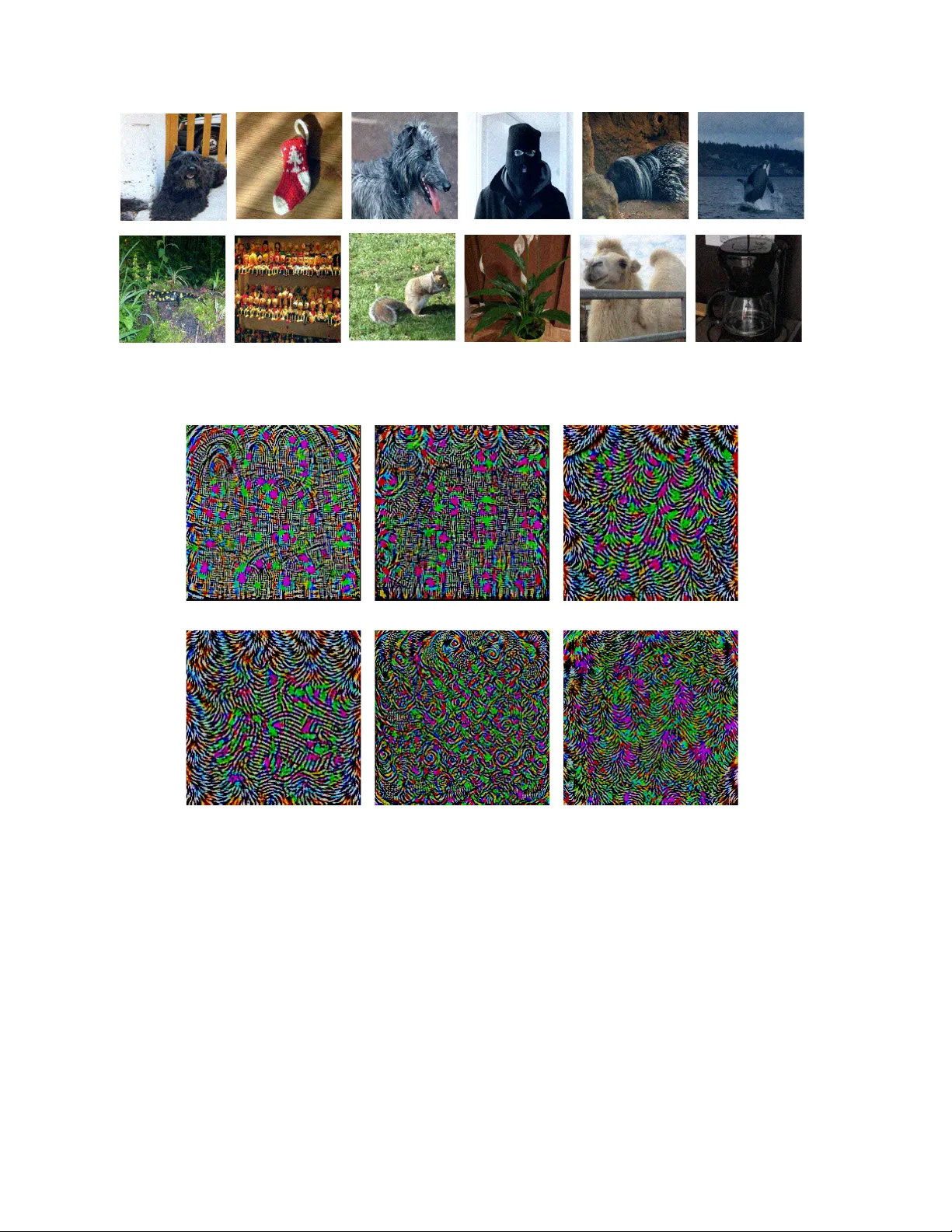
Univ ersal adversarial perturbations Seyed-Mohsen Moosa vi-Dezfooli ∗ † seyed.moosavi@epfl.ch Alhussein Fa wzi ∗ † alhussein.fawzi@epfl.ch Omar Fa wzi ‡ omar.fawzi@ens-lyon.fr Pascal Frossard † pascal.frossard@epfl.ch Abstract Given a state-of-the-art deep neural network classifier , we show the existence of a univer sal (image-a gnostic) and very small perturbation vector that causes natural images to be misclassified with high pr obability . W e pr opose a sys- tematic algorithm for computing universal perturbations, and show that state-of-the-art deep neural networks ar e highly vulner able to such perturbations, albeit being quasi- imper ceptible to the human eye. W e further empirically an- alyze these universal perturbations and show , in particular , that the y g eneralize very well acr oss neural networks. The surprising existence of universal perturbations re veals im- portant geometric corr elations among the high-dimensional decision boundary of classifiers. It further outlines poten- tial security br eaches with the e xistence of single dir ections in the input space that adversaries can possibly exploit to br eak a classifier on most natural ima ges. 1 1. Introduction Can we find a single small image perturbation that fools a state-of-the-art deep neural network classifier on all nat- ural images? W e show in this paper the existence of such quasi-imperceptible univer sal perturbation vectors that lead to misclassify natural images with high probability . Specif- ically , by adding such a quasi-imper ceptible perturbation to natural images, the label estimated by the deep neu- ral network is changed with high probability (see Fig. 1 ). Such perturbations are dubbed universal , as the y are image- agnostic. The existence of these perturbations is problem- atic when the classifier is deployed in real-world (and pos- sibly hostile) en vironments, as they can be e xploited by ad- ∗ The first two authors contributed equally to this w ork. † ´ Ecole Polytechnique F ´ ed ´ erale de Lausanne, Switzerland ‡ ENS de L yon, LIP , UMR 5668 ENS L yon - CNRS - UCBL - INRIA, Univ ersit ´ e de L yon, France 1 T o encourage reproducible research, the code is av ailable at gitHub . Furthermore, a video demonstrating the effect of universal perturbations on a smartphone can be found here . J o y s t i c k W h i p t a i l l iz a r d B al lo o n Ly caenid Tibetan masti T h r e s h e r G ri l l e F l a g p o l e F a c e p o w d e r Labrador C h i h u a h u a C h i h u a h u a J a y L a b r a d o r L a b r a d o r Tibetan masti Brabancon grion Border terrier Figure 1: When added to a natural image, a universal per- turbation image causes the image to be misclassified by the deep neural network with high probability . Left images: Original natural images. The labels are shown on top of each arrow . Central image: Uni versal perturbation. Right images: Perturbed images. The estimated labels of the per- turbed images are shown on top of each arro w . 1 versaries to break the classifier . Indeed, the perturbation process inv olves the mere addition of one very small pertur- bation to all natural images, and can be relativ ely straight- forward to implement by adv ersaries in real-world en viron- ments, while being relativ ely difficult to detect as such per- turbations are very small and thus do not significantly af fect data distributions. The surprising existence of universal per - turbations further reveals new insights on the topology of the decision boundaries of deep neural networks. W e sum- marize the main contributions of this paper as follo ws: • W e show the existence of uni versal image-agnostic perturbations for state-of-the-art deep neural networks. • W e propose an algorithm for finding such perturba- tions. The algorithm seeks a uni versal perturbation for a set of training points, and proceeds by aggregating atomic perturbation vectors that send successive data- points to the decision boundary of the classifier . • W e show that uni versal perturbations hav e a remark- able generalization property , as perturbations com- puted for a rather small set of training points fool new images with high probability . • W e show that such perturbations are not only univer - sal across images, b ut also generalize well across deep neural networks. Such perturbations are therefore dou- bly uni v ersal, both with respect to the data and the net- work architectures. • W e explain and analyze the high vulnerability of deep neural networks to universal perturbations by examin- ing the geometric correlation between different parts of the decision boundary . The robustness of image classifiers to structured and un- structured perturbations hav e recently attracted a lot of at- tention [ 19 , 16 , 20 , 3 , 4 , 12 , 13 , 14 ]. Despite the impressi ve performance of deep neural network architectures on chal- lenging visual classification benchmarks [ 6 , 9 , 21 , 10 ], these classifiers were shown to be highly vulnerable to perturba- tions. In [ 19 ], such networks are shown to be unstable to very small and often imperceptible additiv e adversarial per- turbations. Such carefully crafted perturbations are either estimated by solving an optimization problem [ 19 , 11 , 1 ] or through one step of gradient ascent [ 5 ], and result in a perturbation that fools a specific data point. A fundamental property of these adversarial perturbations is their intrin- sic dependence on datapoints: the perturbations are specif- ically crafted for each data point independently . As a re- sult, the computation of an adversarial perturbation for a new data point requires solving a data-dependent optimiza- tion problem from scratch, which uses the full knowledge of the classification model. This is different from the uni- versal perturbation considered in this paper , as we seek a single perturbation v ector that fools the netw ork on most natural images. Perturbing a new datapoint then only in- volv es the mere addition of the univ ersal perturbation to the image (and does not require solving an optimization prob- lem/gradient computation). Finally , we emphasize that our notion of uni versal perturbation dif fers from the general- ization of adversarial perturbations studied in [ 19 ], where perturbations computed on the MNIST task were shown to generalize well across different models. Instead, we exam- ine the existence of uni versal perturbations that are common to most data points belonging to the data distribution. 2. Universal perturbations W e formalize in this section the notion of univ ersal per- turbations, and propose a method for estimating such per- turbations. Let µ denote a distribution of images in R d , and ˆ k define a classification function that outputs for each im- age x ∈ R d an estimated label ˆ k ( x ) . The main focus of this paper is to seek perturbation vectors v ∈ R d that fool the classifier ˆ k on almost all datapoints sampled from µ . That is, we seek a vector v such that ˆ k ( x + v ) 6 = ˆ k ( x ) for “most” x ∼ µ. W e coin such a perturbation universal , as it represents a fixed image-agnostic perturbation that causes label change for most images sampled from the data distribution µ . W e focus here on the case where the distribution µ represents the set of natural images, hence containing a huge amount of v ariability . In that context, we examine the existence of small univ ersal perturbations (in terms of the ` p norm with p ∈ [1 , ∞ ) ) that misclassify most images. The goal is there- fore to find v that satisfies the following two constraints: 1. k v k p ≤ ξ , 2. P x ∼ µ  ˆ k ( x + v ) 6 = ˆ k ( x )  ≥ 1 − δ. The parameter ξ controls the magnitude of the perturbation vector v , and δ quantifies the desired fooling rate for all images sampled from the distribution µ . Algorithm. Let X = { x 1 , . . . , x m } be a set of images sampled from the distribution µ . Our proposed algorithm seeks a universal perturbation v , such that k v k p ≤ ξ , while fooling most data points in X . The algorithm proceeds it- erativ ely ov er the data points in X and gradually builds the univ ersal perturbation, as illustrated in Fig. 2 . At each iter- ation, the minimal perturbation ∆ v i that sends the current perturbed point, x i + v , to the decision boundary of the clas- sifier is computed, and aggregated to the current instance of the uni versal perturbation. In more details, provided the current univ ersal perturbation v does not fool data point x i , we seek the extra perturbation ∆ v i with minimal norm that allows to fool data point x i by solving the following opti- ∆ v 1 x 1,2,3 R 1 R 2 v ∆ v 2 R 3 Figure 2: Schematic representation of the proposed algo- rithm used to compute univ ersal perturbations. In this il- lustration, data points x 1 , x 2 and x 3 are super -imposed, and the classification regions R i (i.e., regions of constant esti- mated label) are sho wn in dif ferent colors. Our algorithm proceeds by aggregating sequentially the minimal perturba- tions sending the current perturbed points x i + v outside of the corresponding classification region R i . mization problem: ∆ v i ← arg min r k r k 2 s.t. ˆ k ( x i + v + r ) 6 = ˆ k ( x i ) . (1) T o ensure that the constraint k v k p ≤ ξ is satisfied, the up- dated universal perturbation is further projected on the ` p ball of radius ξ and centered at 0 . That is, let P p,ξ be the projection operator defined as follows: P p,ξ ( v ) = arg min v 0 k v − v 0 k 2 subject to k v 0 k p ≤ ξ . Then, our update rule is giv en by v ← P p,ξ ( v + ∆ v i ) . Sev- eral passes on the data set X are performed to improv e the quality of the uni versal perturbation. The algorithm is ter- minated when the empirical “fooling rate” on the perturbed data set X v := { x 1 + v , . . . , x m + v } exceeds the target threshold 1 − δ . That is, we stop the algorithm whenev er Err ( X v ) := 1 m m X i =1 1 ˆ k ( x i + v ) 6 = ˆ k ( x i ) ≥ 1 − δ. The detailed algorithm is provided in Algorithm 1 . Interest- ingly , in practice, the number of data points m in X need not be lar ge to compute a uni versal perturbation that is v alid for the whole distrib ution µ . In particular , we can set m to be much smaller than the number of training points (see Section 3 ). The proposed algorithm in volv es solving at most m in- stances of the optimization problem in Eq. ( 1 ) for each pass. While this optimization problem is not conv e x when ˆ k is a Algorithm 1 Computation of univ ersal perturbations. 1: input: Data points X , classifier ˆ k , desired ` p norm of the perturbation ξ , desired accuracy on perturbed sam- ples δ . 2: output: Univ ersal perturbation vector v . 3: Initialize v ← 0 . 4: while Err ( X v ) ≤ 1 − δ do 5: for each datapoint x i ∈ X do 6: if ˆ k ( x i + v ) = ˆ k ( x i ) then 7: Compute the minimal perturbation that sends x i + v to the decision boundary: ∆ v i ← arg min r k r k 2 s.t. ˆ k ( x i + v + r ) 6 = ˆ k ( x i ) . 8: Update the perturbation: v ← P p,ξ ( v + ∆ v i ) . 9: end if 10: end f or 11: end while standard classifier (e.g., a deep neural network), several ef- ficient approximate methods hav e been devised for solving this problem [ 19 , 11 , 7 ]. W e use in the follo wing the ap- proach in [ 11 ] for its efficenc y . It should further be noticed that the objecti ve of Algorithm 1 is not to find the smallest univ ersal perturbation that fools most data points sampled from the distribution, but rather to find one such perturba- tion with sufficiently small norm. In particular, dif ferent random shufflings of the set X naturally lead to a diverse set of universal perturbations v satisfying the required con- straints. The proposed algorithm can therefore be lev eraged to generate multiple univ ersal perturbations for a deep neu- ral network (see next section for visual e xamples). 3. Universal perturbations for deep nets W e no w analyze the robustness of state-of-the-art deep neural network classifiers to universal perturbations using Algorithm 1 . In a first experiment, we assess the estimated univ ersal perturbations for different recent deep neural networks on the ILSVRC 2012 [ 15 ] validation set (50,000 images), and report the fooling ratio , that is the proportion of images that change labels when perturbed by our univ ersal perturbation. Results are reported for p = 2 and p = ∞ , where we respectiv ely set ξ = 2000 and ξ = 10 . These numerical values were chosen in order to obtain a perturbation whose norm is significantly smaller than the image norms, such that the perturbation is quasi-imperceptible when added to CaffeNet [ 8 ] VGG-F [ 2 ] VGG-16 [ 17 ] VGG-19 [ 17 ] GoogLeNet [ 18 ] ResNet-152 [ 6 ] ` 2 X 85.4% 85.9% 90.7% 86.9% 82.9% 89.7% V al. 85.6 87.0% 90.3% 84.5% 82.0% 88.5% ` ∞ X 93.1% 93.8% 78.5% 77.8% 80.8% 85.4% V al. 93.3% 93.7% 78.3% 77.8% 78.9% 84.0% T able 1: Fooling ratios on the set X , and the validation set. natural images 2 . Results are listed in T able 1 . Each result is reported on the set X , which is used to compute the per- turbation, as well as on the validation set (that is not used in the process of the computation of the universal pertur- bation). Observe that for all networks, the uni v ersal per- turbation achieves very high fooling rates on the validation set. Specifically , the univ ersal perturbations computed for CaffeNet and VGG-F fool more than 90% of the validation set (for p = ∞ ). In other words, for any natural image in the validation set, the mere addition of our universal per- turbation fools the classifier more than 9 times out of 10 . This result is moreover not specific to such architectures, as we can also find uni versal perturbations that cause V GG, GoogLeNet and ResNet classifiers to be fooled on natural images with probability edging 80% . These results have an element of surprise, as they show the existence of single univ ersal perturbation vectors that cause natural images to be misclassified with high probability , albeit being quasi- imperceptible to humans. T o verify this latter claim, we show visual examples of perturbed images in Fig. 3 , where the GoogLeNet architecture is used. These images are ei- ther taken from the ILSVRC 2012 validation set, or cap- tured using a mobile phone camera. Observe that in most cases, the univ ersal perturbation is quasi-imper ceptible , yet this po werful image-agnostic perturbation is able to mis- classify any image with high probability for state-of-the-art classifiers. W e refer to the supp. material for the original (unperturbed) images, as well as their ground truth labels. W e also refer to the video in the supplementary material for real-world examples on a smartphone. W e visualize the uni- versal perturbations corresponding to different networks in Fig. 4 . It should be noted that such uni versal perturbations are not unique, as many different uni versal perturbations (all satisfying the two required constraints) can be generated for the same network. In Fig. 5 , we visualize fiv e different univ ersal perturbations obtained by using different random shufflings in X . Observe that such universal perturbations are dif ferent, although they exhibit a similar pattern. This is moreover confirmed by computing the normalized inner products between two pairs of perturbation images, as the normalized inner products do not exceed 0 . 1 , which shows that one can find div erse uni versal perturbations. 2 For comparison, the av erage ` 2 and ` ∞ norm of an image in the vali- dation set is respectiv ely ≈ 5 × 10 4 and ≈ 250 . While the abov e uni versal perturbations are computed for a set X of 10,000 images from the training set (i.e., in av erage 10 images per class), we now examine the influence of the size of X on the quality of the uni versal perturbation. W e show in Fig. 6 the fooling rates obtained on the val- idation set for different sizes of X for GoogLeNet. Note for example that with a set X containing only 500 images, we can fool more than 30% of the images on the validation set. This result is significant when compared to the num- ber of classes in ImageNet ( 1000 ), as it sho ws that we can fool a lar ge set of unseen images, e ven when using a set X containing less than one image per class! The universal perturbations computed using Algorithm 1 hav e therefore a remarkable generalization power over unseen data points, and can be computed on a very small set of training images. Cross-model universality . While the computed pertur- bations are uni versal across unseen data points, we no w e x- amine their cr oss-model universality . That is, we study to which e xtent universal perturbations computed for a spe- cific architecture (e.g., VGG-19) are also valid for another architecture (e.g., GoogLeNet). T able 2 displays a matrix summarizing the universality of such perturbations across six different architectures. For each architecture, we com- pute a universal perturbation and report the fooling ratios on all other architectures; we report these in the rows of T able 2 . Observe that, for some architectures, the universal pertur- bations generalize very well across other architectures. For example, universal perturbations computed for the V GG-19 network hav e a fooling ratio above 53% for all other tested architectures. This result sho ws that our universal perturba- tions are, to some extent, doubly-universal as they general- ize well across data points and very different architectures. It should be noted that, in [ 19 ], adversarial perturbations were previously shown to generalize well, to some extent, across dif ferent neural networks on the MNIST problem. Our results are howe ver different, as we show the general- izability of uni versal perturbations across different architec- tures on the ImageNet data set. This result shows that such perturbations are of practical relevance, as they generalize well across data points and architectures. In particular , in order to fool a ne w image on an unkno wn neural network, a simple addition of a univ ersal perturbation computed on the VGG-19 architecture is likely to misclassify the data point. wool Indian elephant Indian elephant African grey tabby African grey common newt carousel grey fox macaw three-toed sloth macaw Figure 3: Examples of perturbed images and their corresponding labels. The first 8 images belong to the ILSVRC 2012 validation set, and the last 4 are images tak en by a mobile phone camera. See supp. material for the original images. (a) CaffeNet (b) VGG-F (c) VGG-16 (d) VGG-19 (e) GoogLeNet (f) ResNet-152 Figure 4: Uni versal perturbations computed for different deep neural network architectures. Images generated with p = ∞ , ξ = 10 . The pixel v alues are scaled for visibility . V isualization of the effect of univ ersal perturbations. T o gain insights on the ef fect of universal perturbations on natural images, we now visualize the distribution of labels on the ImageNet validation set. Specifically , we build a di- rected graph G = ( V , E ) , whose vertices denote the labels, and directed edges e = ( i → j ) indicate that the majority of images of class i are fooled into label j when applying the univ ersal perturbation. The existence of edges i → j therefore suggests that the preferred fooling label for im- ages of class i is j . W e construct this graph for GoogLeNet, and visualize the full graph in the supp. material for space constraints. The visualization of this graph shows a very pe- culiar topology . In particular , the graph is a union of disjoint components, where all edges in one component mostly con- nect to one tar get label. See Fig. 7 for an illustration of two connected components. This visualization clearly shows the existence of se veral dominant labels , and that universal per- turbations mostly make natural images classified with such Figure 5: Diversity of uni versal perturbations for the GoogLeNet architecture. The fiv e perturbations are generated using different random shufflings of the set X . Note that the normalized inner products for any pair of univ ersal perturbations does not exceed 0 . 1 , which highlights the di v ersity of such perturbations. VGG-F CaffeNet GoogLeNet VGG-16 VGG-19 ResNet-152 VGG-F 93.7% 71.8% 48.4% 42.1% 42.1% 47.4 % CaffeNet 74.0% 93.3% 47.7% 39.9% 39.9% 48.0% GoogLeNet 46.2% 43.8% 78.9% 39.2% 39.8% 45.5% VGG-16 63.4% 55.8% 56.5% 78.3% 73.1% 63.4% VGG-19 64.0% 57.2% 53.6% 73.5% 77.8% 58.0% ResNet-152 46.3% 46.3% 50.5% 47.0% 45.5% 84.0% T able 2: Generalizability of the univ ersal perturbations across dif ferent networks. The percentages indicate the fooling rates. The ro ws indicate the architecture for which the universal perturbations is computed, and the columns indicate the architecture for which the fooling rate is reported. Number of images in X 500 1000 2000 4000 Fooling ratio (%) 0 10 20 30 40 50 60 70 80 90 Figure 6: Fooling ratio on the v alidation set v ersus the size of X . Note that e ven when the univ ersal perturbation is computed on a very small set X (compared to training and validation sets), the fooling ratio on v alidation set is large. labels. W e hypothesize that these dominant labels occupy large regions in the image space, and therefore represent good candidate labels for fooling most natural images. Note that these dominant labels are automatically found by Algo- rithm 1 , and are not imposed a priori in the computation of perturbations. Fine-tuning with universal perturbations. W e now ex- amine the effect of fine-tuning the networks with perturbed images. W e use the VGG-F architecture, and fine-tune the network based on a modified training set where universal perturbations are added to a fraction of (clean) training sam- ples: for each training point, a uni v ersal perturbation is added with probability 0 . 5 , and the original sample is pre- served with probability 0 . 5 . 3 T o account for the di versity of uni versal perturbations, we pre-compute a pool of 10 dif- ferent univ ersal perturbations and add perturbations to the training samples randomly from this pool. The network is fine-tuned by performing 5 extra epochs of training on the modified training set. T o assess the effect of fine-tuning on the robustness of the network, we compute a new universal perturbation for the fine-tuned network (using Algorithm 1 , with p = ∞ and ξ = 10 ), and report the fooling rate of the network. After 5 extra epochs, the fooling rate on the vali- dation set is 76 . 2% , which sho ws an improv ement with re- spect to the original network ( 93 . 7% , see T able 1 ). 4 Despite this improvement, the fine-tuned network remains lar gely vulnerable to small univ ersal perturbations. W e therefore 3 In this fine-tuning experiment, we use a slightly modified notion of univ ersal perturbations, where the dir ection of the universal vector v is fixed for all data points, while its magnitude is adaptive. That is, for each data point x , we consider the perturbed point x + αv , where α is the small- est coefficient that fools the classifier . W e observed that this feedbacking strategy is less prone to overfitting than the strategy where the univ ersal perturbation is simply added to all training points. 4 This fine-tuning procedure moreover led to a minor increase in the error rate on the validation set, which might be due to a slight overfitting of the perturbed data. great grey owl platypus nematode dowitcher Arctic fox leopard digital clock fountain slide rule space shuttle cash machine pillow computer keyboard dining table envelope medicine chest microwave mosquito net pencil box plate rack quilt refrigerator television tray wardrobe window shade Figure 7: T wo connected components of the graph G = ( V , E ) , where the vertices are the set of labels, and directed edges i → j indicate that most images of class i are fooled into class j . repeated the above procedure (i.e., computation of a pool of 10 universal perturbations for the fine-tuned network, fine- tuning of the new network based on the modified training set for 5 extra epochs), and we obtained a new fooling ra- tio of 80 . 0% . In general, the repetition of this procedure for a fixed number of times did not yield any improvement ov er the 76 . 2% fooling ratio obtained after one step of fine- tuning. Hence, while fine-tuning the network leads to a mild improv ement in the robustness, we observed that this sim- ple solution does not fully immune against small univ ersal perturbations. 4. Explaining the vulnerability to universal perturbations The goal of this section is to analyze and explain the high vulnerability of deep neural netw ork classifiers to univer - sal perturbations. T o understand the unique characteristics of uni versal perturbations, we first compare such perturba- tions with other types of perturbations, namely i) random perturbation, ii) adversarial perturbation computed for a randomly picked sample (computed using the DF and FGS methods respectively in [ 11 ] and [ 5 ]), iii) sum of adversar- ial perturbations o ver X , and i v) mean of the images (or ImageNet bias ). For each perturbation, we depict a phase transition graph in Fig. 8 showing the fooling rate on the validation set with respect to the ` 2 norm of the perturba- tion. Dif ferent perturbation norms are achieved by scaling accordingly each perturbation with a multiplicative factor to hav e the target norm. Note that the universal perturbation is computed for ξ = 2000 , and also scaled accordingly . Observe that the proposed univ ersal perturbation quickly reaches very high fooling rates, ev en when the perturbation is constrained to be of small norm. For example, the uni- versal perturbation computed using Algorithm 1 achiev es a fooling rate of 85% when the ` 2 norm is constrained to ξ = 2000 , while other perturbations achiev e much smaller ratios for comparable norms. In particular , random vec- tors sampled uniformly from the sphere of radius of 2000 only fool 10% of the validation set. The large difference between universal and random perturbations suggests that the uni versal perturbation e xploits some geometric corr ela- tions between different parts of the decision boundary of the classifier . In fact, if the orientations of the decision bound- ary in the neighborhood of different data points were com- pletely uncorrelated (and independent of the distance to the decision boundary), the norm of the best univ ersal perturba- tion would be comparable to that of a random perturbation. Note that the latter quantity is well understood (see [ 4 ]), as the norm of the random perturbation required to fool a specific data point precisely behaves as Θ( √ d k r k 2 ) , where d is the dimension of the input space, and k r k 2 is the dis- tance between the data point and the decision boundary (or equiv alently , the norm of the smallest adversarial perturba- tion). For the considered ImageNet classification task, this quantity is equal to √ d k r k 2 ≈ 2 × 10 4 , for most data points, which is at least one order of magnitude lar ger than the uni- versal perturbation ( ξ = 2000 ). This substantial difference between random and universal perturbations thereby sug- gests redundancies in the geometry of the decision bound- aries that we now e xplore. For each image x in the validation set, we com- pute the adversarial perturbation vector r ( x ) = arg min r k r k 2 s.t. ˆ k ( x + r ) 6 = ˆ k ( x ) . It is easy to see that r ( x ) is normal to the decision boundary of the clas- sifier (at x + r ( x ) ). The vector r ( x ) hence captures the local geometry of the decision boundary in the region surrounding the data point x . T o quantify the correlation 0 2000 4000 6000 8000 10000 Norm of perturbation 0 0.1 0.2 0.3 0.4 0.5 0.6 0.7 0.8 0.9 1 Fooling rate Universal Random Adv. pert. (DF) Adv. pert. (FGS) Sum ImageNet bias Figure 8: Comparison between fooling rates of different perturbations. Experiments performed on the CaffeNet ar- chitecture. between different regions of the decision boundary of the classifier , we define the matrix N =  r ( x 1 ) k r ( x 1 ) k 2 . . . r ( x n ) k r ( x n ) k 2  of normal vectors to the decision boundary in the vicinity of n data points in the validation set. For binary linear classifiers, the decision boundary is a hyperplane, and N is of rank 1 , as all normal vectors are collinear . T o capture more generally the correlations in the decision boundary of complex classifiers, we compute the singular values of the matrix N . The singular values of the matrix N , computed for the Caf feNet architecture are shown in Fig. 9 . W e fur- ther show in the same figure the singular values obtained when the columns of N are sampled uniformly at random from the unit sphere. Observe that, while the latter singu- lar values hav e a slo w decay , the singular values of N de- cay quickly , which confirms the existence of large corre- lations and redundancies in the decision boundary of deep networks. More precisely , this suggests the existence of a subspace S of low dimension d 0 (with d 0  d ), that contains most normal vectors to the decision boundary in re gions surrounding natural images. W e hypothesize that the exis- tence of univ ersal perturbations fooling most natural images is partly due to the existence of such a low-dimensional sub- space that captures the correlations among different re gions of the decision boundary . In fact, this subspace “collects” normals to the decision boundary in different regions, and perturbations belonging to this subspace are therefore likely to fool datapoints. T o verify this hypothesis, we choose a random vector of norm ξ = 2000 belonging to the subspace S spanned by the first 100 singular vectors, and compute its fooling ratio on a different set of images (i.e., a set of images that hav e not been used to compute the SVD). Such a pertur- bation can fool nearly 38% of these images, thereby sho w- ing that a random direction in this well-sought subspace S significantly outperforms random perturbations (we recall 0 0.5 1 1.5 2 2.5 3 3.5 4 4.5 5 Index 10 4 0 0.5 1 1.5 2 2.5 3 3.5 4 4.5 5 Singular values Random Normal vectors Figure 9: Singular values of matrix N containing normal vectors to the decision decision boundary . Figure 10: Illustration of the lo w dimensional subspace S containing normal vectors to the decision boundary in regions surrounding natural images. For the purpose of this illustration, we super-impose three data-points { x i } 3 i =1 , and the adversarial perturbations { r i } 3 i =1 that send the re- spectiv e datapoints to the decision boundary { B i } 3 i =1 are shown. Note that { r i } 3 i =1 all liv e in the subspace S . that such perturbations can only fool 10% of the data). Fig. 10 illustrates the subspace S that captures the correlations in the decision boundary . It should further be noted that the existence of this low dimensional subspace e xplains the sur- prising generalization properties of univ ersal perturbations obtained in Fig. 6 , where one can build relativ ely general- izable univ ersal perturbations with v ery few images. Unlike the above e xperiment, the proposed algorithm does not choose a random vector in this subspace, but rather chooses a specific direction in order to maximize the over - all fooling rate. This explains the gap between the fooling rates obtained with the random v ector strate gy in S and Al- gorithm 1 . 5. Conclusions W e showed the existence of small univ ersal perturba- tions that can fool state-of-the-art classifiers on natural im- ages. W e proposed an iterativ e algorithm to generate uni- versal perturbations, and highlighted se veral properties of such perturbations. In particular, we showed that univ ersal perturbations generalize well across different classification models, resulting in doubly-univ ersal perturbations (image- agnostic, network-agnostic). W e further explained the ex- istence of such perturbations with the correlation between different regions of the decision boundary . This provides insights on the geometry of the decision boundaries of deep neural networks, and contributes to a better understanding of such systems. A theoretical analysis of the geometric correlations between dif ferent parts of the decision bound- ary will be the subject of future research. Acknowledgments W e gratefully acknowledge the support of NVIDIA Cor- poration with the donation of the T esla K40 GPU used for this research. References [1] O. Bastani, Y . Ioannou, L. Lampropoulos, D. Vytiniotis, A. Nori, and A. Criminisi. Measuring neural net robustness with constraints. In Neural Information Pr ocessing Systems (NIPS) , 2016. 2 [2] K. Chatfield, K. Simonyan, A. V edaldi, and A. Zisserman. Return of the devil in the details: Delving deep into conv o- lutional nets. In British Machine V ision Conference , 2014. 4 [3] A. Fawzi, O. Fa wzi, and P . Frossard. Analysis of clas- sifiers’ robustness to adversarial perturbations. CoRR , abs/1502.02590, 2015. 2 [4] A. Fa wzi, S. Moosavi-Dezfooli, and P . Frossard. Robustness of classifiers: from adversarial to random noise. In Neural Information Pr ocessing Systems (NIPS) , 2016. 2 , 7 [5] I. J. Goodfellow , J. Shlens, and C. Szegedy . Explaining and harnessing adversarial examples. In International Confer- ence on Learning Repr esentations (ICLR) , 2015. 2 , 7 [6] K. He, X. Zhang, S. Ren, and J. Sun. Deep residual learning for image recognition. In IEEE Conference on Computer V ision and P attern Recognition (CVPR) , 2016. 2 , 4 [7] R. Huang, B. Xu, D. Schuurmans, and C. Szepesv ´ ari. Learn- ing with a strong adversary . CoRR, abs/1511.03034 , 2015. 3 [8] Y . Jia, E. Shelhamer, J. Donahue, S. Karayev , J. Long, R. Gir- shick, S. Guadarrama, and T . Darrell. Caffe: Conv olu- tional architecture for fast feature embedding. In A CM Inter- national Confer ence on Multimedia (MM) , pages 675–678, 2014. 4 [9] A. Krizhevsk y , I. Sutskev er , and G. E. Hinton. Imagenet classification with deep con v olutional neural networks. In Advances in neural information processing systems (NIPS) , pages 1097–1105, 2012. 2 [10] Q. V . Le, W . Y . Zou, S. Y . Y eung, and A. Y . Ng. Learn- ing hierarchical in variant spatio-temporal features for action recognition with independent subspace analysis. In Com- puter V ision and P attern Recognition (CVPR), 2011 IEEE Confer ence on , pages 3361–3368. IEEE, 2011. 2 [11] S.-M. Moosavi-Dezfooli, A. Fawzi, and P . Frossard. Deep- fool: a simple and accurate method to fool deep neural net- works. In IEEE Confer ence on Computer V ision and P attern Recognition (CVPR) , 2016. 2 , 3 , 7 [12] A. Nguyen, J. Y osinski, and J. Clune. Deep neural networks are easily fooled: High confidence predictions for unrecog- nizable images. In IEEE Confer ence on Computer V ision and P attern Recognition (CVPR) , pages 427–436, 2015. 2 [13] E. Rodner, M. Simon, R. Fisher , and J. Denzler . Fine-grained recognition in the noisy wild: Sensitivity analysis of con- volutional neural networks approaches. In British Machine V ision Confer ence (BMVC) , 2016. 2 [14] A. Rozsa, E. M. Rudd, and T . E. Boult. Adv ersarial di- versity and hard positive generation. In IEEE Confer ence on Computer V ision and P attern Recognition (CVPR) W ork- shops , 2016. 2 [15] O. Russako vsky , J. Deng, H. Su, J. Krause, S. Satheesh, S. Ma, Z. Huang, A. Karpathy , A. Khosla, M. Bernstein, A. Berg, and L. Fei-Fei. Imagenet large scale visual recog- nition challenge. International Journal of Computer V ision , 115(3):211–252, 2015. 3 [16] S. Sabour , Y . Cao, F . Faghri, and D. J. Fleet. Adversarial manipulation of deep representations. In International Con- fer ence on Learning Repr esentations (ICLR) , 2016. 2 [17] K. Simonyan and A. Zisserman. V ery deep conv olutional networks for large-scale image recognition. In International Confer ence on Learning Repr esentations (ICLR) , 2014. 4 [18] C. Szegedy , W . Liu, Y . Jia, P . Sermanet, S. Reed, D. Anguelov , D. Erhan, V . V anhoucke, and A. Rabinovich. Going deeper with con volutions. In IEEE Conference on Computer V ision and P attern Recognition (CVPR) , 2015. 4 [19] C. Szegedy , W . Zaremba, I. Sutskever , J. Bruna, D. Erhan, I. Goodfello w , and R. Fer gus. Intriguing properties of neural networks. In International Confer ence on Learning Repr e- sentations (ICLR) , 2014. 2 , 3 , 4 [20] P . T abacof and E. V alle. Exploring the space of adversar- ial images. IEEE International Joint Confer ence on Neural Networks , 2016. 2 [21] Y . T aigman, M. Y ang, M. Ranzato, and L. W olf. Deepface: Closing the gap to human-level performance in f ace v erifica- tion. In IEEE Conference on Computer V ision and P attern Recognition (CVPR) , pages 1701–1708, 2014. 2 A. A ppendix Fig. 11 shows the original images corresponding to the experiment in Fig. 3 . Fig. 12 visualizes the graph showing relations between original and perturbed labels (see Section 3 for more details). Bouvier des Flandres Christmas stocking Scottish deerhound ski mask porcupine killer whale European fire salamander toyshop fox squirrel pot Arabian camel coffeepot Figure 11: Original images. The first two rows are randomly chosen images from the validation set, and the last row of images are personal images taken from a mobile phone camera. great grey owl platypus nematode dowitcher Arctic fox leopard digital clock fountain slide rule space shuttle junco common iguana axolotl tree frog banded gecko American chameleon green lizard African chameleon African crocodile water snake green mamba cougar rhinoceros beetle weevil grasshopper cricket walking stick mantis lacewing Band Aid cliff dwelling hammer photocopier tank tub dough burrito green snake tick long-horned beetle night snake house �inch African grey chickadee water ouzel kite black and gold garden spider garden spider sulphur-crested cockatoo conch hermit crab white stork ruddy turnstone red-backed sandpiper oystercatcher albatross grey whale killer whale Maltese dog Pekinese Walker hound Lhasa schipperke Eskimo dog Great Pyrenees Samoyed Pembroke toy poodle Persian cat ice bear hartebeest llama sturgeon abaya acoustic guitar aircraft carrier airliner airship amphibian assault ri�le backpack balance beam balloon ballpoint bannister barbell barbershop barn bassoon bathtub beacon bell cote bikini binoculars boathouse bobsled bow tie brassiere breakwater breastplate bucket caldron cannon can opener car mirror carton cassette player castle catamaran CD player chime church cleaver cocktail shaker container ship convertible corkscrew cornet cowboy hat cradle crane dam desk desktop computer diaper dock dogsled drilling platform drum drumstick dumbbell espresso maker �ireboat �lagpole �lute folding chair fountain pen frying pan garbage truck gasmask golf ball gown grand piano guillotine hair spray hand blower harmonica harvester home theater hook iPod iron joystick knee pad lab coat ladle letter opener lifeboat liner Loafer loudspeaker loupe maillot measuring cup megalith microphone military uniform missile mixing bowl mobile home modem monastery mortarboard mosque mountain tent mouse mousetrap moving van muzzle nail nipple oboe oxygen mask paintbrush palace paper towel passenger car patio pedestal pencil sharpener Petri dish pier ping-pong ball pirate plane planetarium plastic bag plunger Polaroid camera pole pool table power drill printer projectile projector punching bag purse quill racket radiator radio telescope re�lex camera rubber eraser saltshaker sandal scale screwdriver seat belt shoji ski sliding door snowmobile snowplow soap dispenser solar dish space heater spatula speedboat spotlight steam locomotive steel arch bridge stethoscope strainer studio couch stupa submarine suit sunglass sunscreen suspension bridge swimming trunks switch syringe table lamp teapot thatch toaster trailer truck trench coat trimaran tripod turnstile vacuum vase viaduct violin volleyball warplane washbasin washer water tower whiskey jug whistle wig wing wok worm fence wreck yawl traf�ic light plate consomme ice cream hay chocolate sauce alp cliff geyser lakeside promontory sandbar seashore valley volcano groom toilet tissue great white shark macaw tiger shark hammerhead electric ray stingray gold�inch indigo bunting bulbul jay magpie bald eagle vine snake barn spider bee eater hornbill hummingbird jacamar jelly�ish chambered nautilus American egret dugong Siberian husky ladybug leaf beetle �ly ant lea�hopper dragon�ly damsel�ly admiral cabbage butter�ly sulphur butter�ly lycaenid Angora beer glass candle cinema cloak electric guitar jack-o'-lantern lampshade lens cap lighter matchstick obelisk parachute parallel bars pinwheel ri�le schooner soup bowl stage tennis ball torch upright water jug bell pepper lemon red wine scuba diver ringneck snake banana American lobster cray�ish cockroach Kerry blue terrier giant schnauzer miniature poodle tabby tiger cat Egyptian cat lynx black widow Indian elephant sloth bear African elephant cello crutch fur coat maillot miniskirt neck brace pickelhaube potter's wheel prison sax shovel spindle Crock Pot Dutch oven bulletproof vest cardigan jersey Windsor tie chest chiffonier safe stove crash helmet mask shower cap ski mask sunglasses cash machine pillow computer keyboard dining table envelope medicine chest microwave mosquito net pencil box plate rack quilt refrigerator television tray wardrobe window shade mailbag beaker thimble china cabinet coffee mug coffeepot lipstick oil �ilter perfume wine bottle espresso cup eggnog binder wallet monitor notebook oscilloscope screen tape player barrel wool bath towel broom crate face powder knot lotion maraca mitten mortar pick pill bottle rule sweatshirt velvet wooden spoon ice lolly cheeseburger hotdog spaghetti squash butternut squash Granny Smith strawberry Figure 12: Graph representing the relation between original and perturbed labels. Note that “dominant labels” appear systematically . Please zoom for readability . Isolated nodes are remov ed from this visualization for readability .