Eigenvector statistics of the product of Ginibre matrices

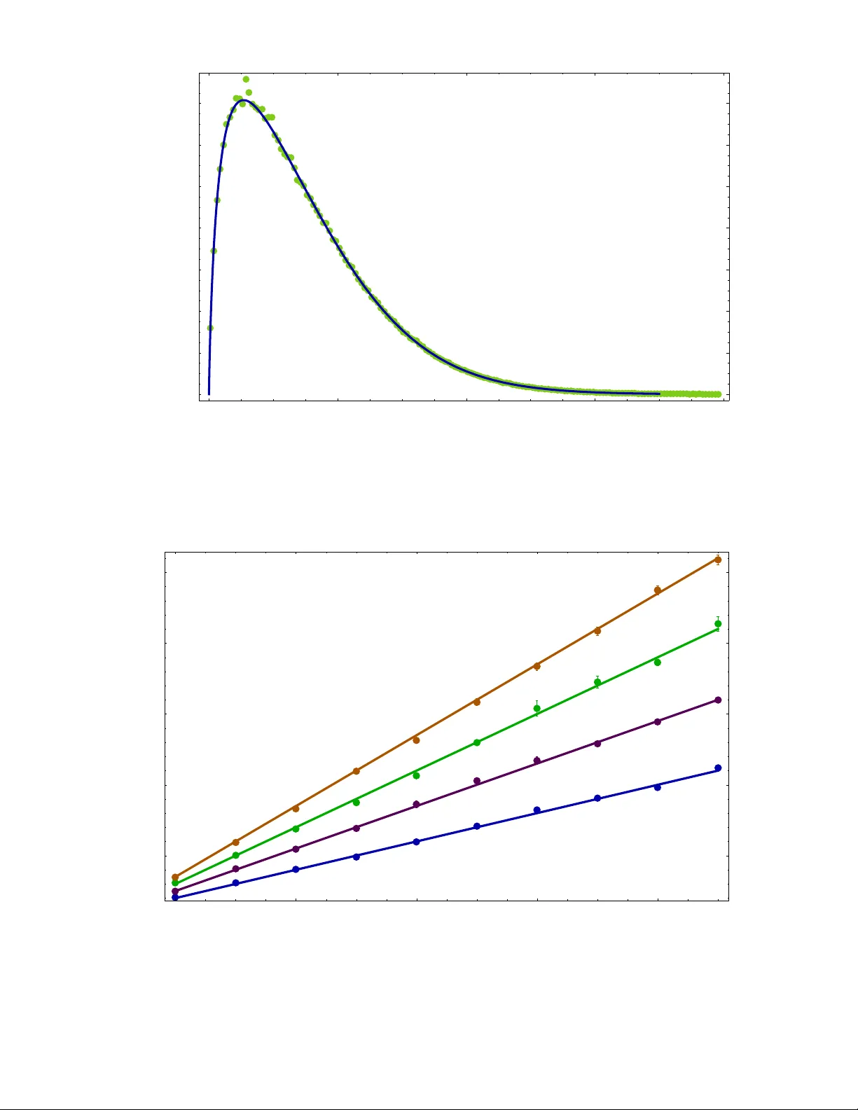
Eigen vector statistics of the product of Ginibre matrices Zdzisław Burda ∗ and Bartłomiej J. Spisak † A GH University of Science and T echnolo gy , F aculty of Physics and Applied Computer Science, al. Mickiewicza 30, 30-059 Krak ´ ow , P oland Pierpaolo V i vo ‡ Department of Mathematics, King’ s Colle ge London, Strand WC2R 2LS, London, U.K. W e dev elop a method to calculate left-right eigen vector correlations of the product of m independent N × N complex Ginibre matrices. For illustration, we present explicit analytical results for the vector o verlap for a couple of examples for small m and N . W e conjecture that the integrated ov erlap between left and right eigen vectors is giv en by the formula O = 1 + ( m/ 2)( N − 1) and support this conjecture by analytical and numerical calculations. W e deri ve an analytical expression for the limiting correlation density as N → ∞ for the product of Ginibre matrices as well as for the product of elliptic matrices. In the latter case, we find that the correlation function is independent of the eccentricities of the elliptic laws. Ke ywords: random matrix theory , non-hermitian, planar diagram enumeration ∗ zdzislaw .burda@agh.edu.pl † bjs@agh.edu.pl ‡ pierpaolo.viv o@kcl.ac.uk 2 I. INTR ODUCTION Products of random matrices have continuously attracted attention since the sixties [1 – 5]. They are of relev ance in many fields of mathematics, physics and engineering including dynamical systems [2, 6], disordered systems [7–9], statistical me- chanics [10], quantum mechanics [11], quantum transport and mesoscopic systems [12, 13], hidden Marko v models [14], image processing [15], quantum chromodynamics [16], wireless telecommunication [17, 18], quantitative finance [19 – 21] and many others [22]. Recently , an enormous progress has been made in the understanding of macroscopic [23–44] and microscopic [45– 66] statistics of eigen values and singular values as well as of L yapunov spectra for products of random matrices [67 – 77]. In contrast, not much has been learned about the eigenv ector statistics of the products of random matrices so far . In this paper , we address this problem by considering a correlation function for eigenv ectors of the product of Ginibre matrices. More precisely , we study the o verlap between left and right eigen vectors for finite N and for N → ∞ . In the first part of the paper , we adapt ideas dev eloped in [78, 79] to the product of random matrices by using the generalized Schur decomposition [45] for finite N , while in the second part we combine the generalized Green function method [81 – 84] with linearization (subordination) [10, 28, 37] to deriv e the limiting law for the ov erlap for N → ∞ . II. DEFINITIONS Consider a diagonalizable matrix X ov er the field of comple x numbers. Let { Λ α } be the eigen values of X . The corresponding left eigen vectors h L α | and right eigen vectors | R α i satisfy the relations X | R α i = Λ α | R α i , h L α | X = h L α | Λ α . (1) Note that the Hermitian conjugate of the second equation has the form: X † | L α i = ¯ Λ α | L α i , where the symbol ’bar’ denotes the complex conjugation of Λ α . The eigenv ectors fulfill the bi-orthogonality and closure relations in the form h L α | R β i = δ αβ , X α | L α i h R α | = 1 . (2) The two relations are in v ariant with respect to the scale transformation | R α i → c α | R α i , h L α | → h L α | c − 1 α , (3) with arbitrary non-zero coefficients c α ’ s. According to Refs. [78, 79], an overlap of the left and right eigenv ectors is defined in the following w ay O αβ = h L α | L β i h R β | R α i . (4) By construction, the quantity O αβ is in variant with respect to the scale transformation given by Eq. (3) and consequently does not depend on the vector normalizations. If X is a random matrix, one defines av erages over the ensemble h O αβ i = Z dµ ( X ) O αβ , (5) where dµ ( X ) is the probability measure for the random matrix in question. The dependence of O αβ on X is suppressed in the notation. W e use this notation throughout the paper also for other observables that depend on random matrices. The global diagonal ov erlap averaged o ver the ensemble is giv en by O = * 1 N N X α =1 O αα + , (6) while the global off-diagonal one is e xpressed by the formula O of f = * 2 N ( N − 1) X α<β O αβ + . (7) W e are interested here in unitarily in variant random matrices for which the probability measure is in variant with respect to the similarity transformation X → U X U − 1 , where U is a unitary matrix. In particular , this in v ariance implies that h O αα i = h O 11 i and h O αβ i = h O 12 i for any α and β . It follows that O = h O 11 i , O of f = h O 12 i . (8) 3 W e can also define the local diagonal overlap density by the formula O ( z ) = * 1 N N X α =1 O αα δ ( z − Λ α ) + = h O 11 δ ( z − Λ 1 ) i , (9) and the off-diagonal one by O of f ( z , w ) = * 2 N ( N − 1) X α<β O αβ δ ( z − Λ α ) δ ( w − Λ β ) + = h O 12 δ ( z − Λ 1 ) δ ( w − Λ 2 ) i . (10) The symbol δ ( z ) denotes the Dirac delta function on the complex plane. Clearly , the diagonal global overlap is equal to the integrated o verlap density giv en by Eq. (9), i.e. O = Z d 2 z O ( z ) . (11) III. PR ODUCT OF GINIBRE MA TRICES Consider the product X = X 1 X 2 · · · X m (12) of m independent identically distrib uted N × N Ginibre random matrices [85] with complex entries. The probability measure factorizes and can be written as a product of measures for indi vidual Ginibre matrices dµ ( X ) ≡ dµ ( X 1 , X 2 , . . . , X m ) = dµ ( X 1 ) dµ ( X 2 ) · · · dµ ( X m ) , (13) each of which is giv en by dµ ( X i ) =  π σ 2  − N 2 e − 1 σ 2 T r X i X † i D X i , (14) where σ is a scale parameter , and DX i = Q αβ d Re X i,αβ d Im X i,αβ . According to Eq. (9), the local diagonal overlap density can be calculated with respect to the measure dµ ( X ) in the follo wing way O ( z ) = Z dµ ( X ) O 11 δ ( z − Λ 1 ) , (15) where Λ α ’ s correspond to the eigen values of the product X (12). An analogous formula holds for the off-diagonal density . In the calculations we set σ = 1 . One can easily transform the result to other values of σ (14) by using the formula O σ ( z ) = 1 σ 2 m O σ =1  z σ m  , (16) which merely corresponds to the scale transformation of all Ginibre matrices X i − → σ X i in the product (12). Later , when discussing the limiting laws for N → ∞ we will choose σ = N − 1 / 2 . This choice of the scale parameter σ will ensure the existence of the limiting eigen v alue density on a compact support being the unit disk in the complex plane. IV . CALCULA TIONS OF THE O VERLAP FOR FINITE N In order to calculate the global left-right vector overlap, defined by Eq. (4), for the product of Ginibre matrices (12), we will change the parametrization of the matrices X i ’ s using the generalized Schur decomposition [45] X i = U i − 1 τ i U † i , (17) 4 for i = 1 , . . . , m , where U i are unitary matrices from the unitary group U ( N ) , and τ i are upper triangular matrices of size N × N . W e use a cyclic indexing U i ≡ U m + i , in particular U 0 ≡ U m . Sometimes it is conv enient to express each τ i as a sum of a diagonal matrix λ i and a strictly upper triangular one t i , namely τ i = λ i + t i =       λ i, 1 t i, 12 t i, 13 . . . t i, 1 N 0 λ i, 2 t i, 23 . . . t i, 2 N . . . 0 0 0 λ i,N − 1 t i,N − 1 N 0 0 0 . . . λ i,N       . (18) In this representation, the product X is unitarily equiv alent to a matrix T , that is X = U m T U † m , where T = τ 1 τ 2 · · · τ m . (19) The matrix T has also an upper triangular form T = Λ + T =       Λ 1 T 12 T 13 . . . T 1 N 0 Λ 2 T 23 . . . T 2 N . . . 0 0 0 Λ N − 1 T N − 1 N 0 0 0 . . . Λ N       . (20) The diagonal elements of T are giv en by T α ≡ Λ α = λ 1 ,α λ 2 ,α · · · λ m,α , (21) and the off-diagonal ones by T αν = X α ≤ β ≤ ... ≤ ν τ 1 ,αβ τ 2 ,β γ · · · τ m,µν . (22) Any instance of τ i,αα with two identical Greek indices can be replaced by λ i,α and of τ i,αβ with two dif ferent Greek indices by t i,αβ in the last formula. One can also express the integration measure in terms of U ’ s, λ ’ s and t ’ s. Since one is interested in in variant observ ables, the U ’ s can be integrated out. For the scale parameter σ = 1 one gets [45] dµ ( λ, t ) = Z − 1 | ∆ ( Λ ) | 2 Y i,α e −| λ i,α | 2 d 2 λ i,α Y j,β <γ 1 π e −| t j,βγ | 2 d 2 t j,β γ , (23) where the normalization factor Z is given by the formula Z = N ![ π N 1!2! · · · ( N − 1)!] m , (24) and the V andermonde determinant ∆ ( Λ ) for the product X = X 1 X 2 · · · X m has the form ∆ ( Λ ) = Y α<β ( λ 1 ,α λ 2 ,α · · · λ m,α − λ 1 ,β λ 2 ,β · · · λ m,β ) = Y α<β (Λ α − Λ β ) . (25) The square of the determinant in Eq. (23) comes from the Jacobian of the transformation (17). The next step is to express the observ ables in terms of t 0 s and λ 0 s . For e xample, to calculate the diagonal overlap density [cf. Eq. (15)], we hav e to find O 11 = O 11 ( t, λ ) and to inte grate over t ’ s and λ ’ s with the Dirac delta constraint O ( z ) = Z dµ ( λ, t ) O 11 ( t, λ ) δ ( z − Λ 1 ) , (26) while for the global ov erlap O = R dµ ( λ, t ) O 11 ( t, λ ) . The measure dµ ( λ, t ) (23) factorizes dµ ( λ, t ) = dµ ( λ ) dµ ( t ) . One can first integrate over t ’ s. This is a Gaussian integral and can be easily performed. After this integration, only the dependence on λ ’ s is left O 11 ( λ ) = Z dµ ( t ) O 11 ( t, λ ) , (27) 5 where dµ ( t ) is a normalized Gaussian measure equal to the t -dependent piece of dµ ( λ, t ) (23). The last step is to integrate ov er λ ’ s with the measure gi ven by Eq. (23) O ( z ) = Z − 1 Z dµ ( λ ) | ∆ ( Λ ) | 2 e − P i,α | λ i,α | 2 O 11 ( λ ) δ ( z − Λ 1 ) , (28) where as before Λ α ’ s stand for Λ α = λ 1 ,α λ 2 ,α · · · λ m,α . W e will do this below . First we hav e to find the function O 11 ( t, λ ) . This can be done as follows. W e choose the basis in which the product matrix X is equal to T . Such a basis exists since the two matrices are unitarily equiv alent. In this basis, the first right eigen vector | R 1 i is represented as a column vector with ’ 1 ’ in the position 1 and zeros else where: | R 1 i = (1 , 0 , 0 , . . . ) T . The vector is written here as transpose of a row vector to sa ve space. Denote the elements of the first left eigen vector h L 1 | = ( B 1 , B 2 , . . . ) . The eigen value equation h L 1 |T = h L 1 | Λ 1 leads to the following recursion relation for B β ’ s [78, 79] B β = 1 Λ 1 − Λ β β − 1 X α =1 B α T αβ . (29) The recursion is initiated by B 1 = 1 as follo ws from the bi-orthogonality relation (2). One finds B 1 = 1 , B 2 = T 12 Λ 1 − Λ 2 , B 3 = T 13 Λ 1 − Λ 3 + T 12 T 23 (Λ 1 − Λ 2 )(Λ 1 − Λ 3 ) , B 4 = T 14 Λ 1 − Λ 4 + T 12 T 24 (Λ 1 − Λ 2 )(Λ 1 − Λ 4 ) + T 13 T 34 (Λ 1 − Λ 3 )(Λ 1 − Λ 4 ) + + T 12 T 23 T 34 (Λ 1 − Λ 2 )(Λ 1 − Λ 3 )(Λ 1 − Λ 4 ) , etc . (30) The element O 11 of the ov erlap matrix is related to B ’ s as O 11 = N X α =1 | B α | 2 , (31) and B ’ s depend on t ’ s and λ ’ s through T ’ s and Λ ’ s. Combining Eqs. (30),(31) with Eq. (26) we obtain an explicit form of the integral o ver t ’ s and λ ’ s which can be done. W e will give a couple of e xamples below . V . EXAMPLES Let us first illustrate the calculations for N = 2 , m = 2 and σ = 1 - that is for the product of two 2 × 2 Ginibre matrices. Firstly , we express T 12 in terms of t ’ s and λ ’ s as follows T =  λ 1 , 1 t 1 , 12 0 λ 1 , 2   λ 2 , 1 t 2 , 12 0 λ 2 , 2  =  Λ 1 T 12 0 Λ 2  . (32) This giv es T 12 = λ 1 , 1 t 2 , 12 + t 1 , 12 λ 2 , 2 and Λ α = λ 1 ,α λ 2 ,α for α = 1 , 2 . Thus we ha ve O 11 ( t, λ ) = 1 + | T 12 | 2 | Λ 1 − Λ 2 | 2 = 1 + | λ 1 , 1 t 2 , 12 + t 1 , 12 λ 2 , 2 | 2 | λ 1 , 1 λ 2 , 1 − λ 1 , 2 λ 2 , 2 | 2 . (33) According to Eq. (27), the integration o ver t ’ s leads to the follo wing result O 11 ( λ ) = 1 + | λ 1 , 1 | 2 + | λ 2 , 2 | 2 | λ 1 , 1 λ 2 , 1 − λ 1 , 2 λ 2 , 2 | 2 . (34) Now we ha ve to compute the inte gral over λ ’ s given by Eq. (28), namely O ( z ) = 1 2 π 4 Z  | λ 1 , 1 λ 2 , 1 − λ 1 , 2 λ 2 , 2 | 2 + | λ 1 , 1 | 2 + | λ 2 , 2 | 2  δ ( z − λ 1 , 1 λ 2 , 1 ) Y i,α e −| λ i,α | 2 d 2 λ i,α . (35) 6 W e first integrate over the λ ’ s that do not appear in the Dirac delta, that is λ 1 , 2 and λ 2 , 2 . These integrals are in general of the Gaussian type combined with a power function, i.e. R d 2 z | z | 2 k exp ( −| z | 2 ) = π k ! . As a result of the integration, we obtain O ( z ) = 1 2 π 2 Z  | z | 2 + 2 + | λ 1 , 1 | 2  δ ( z − λ 1 , 1 λ 2 , 1 ) e −| λ 1 , 1 | 2 −| λ 2 , 1 | 2 d 2 λ 1 , 1 d 2 λ 2 , 1 . (36) Now we inte grate over λ 2 , 1 . W e use the scaling property of the Dirac delta δ ( a ( z − z 0 )) = (1 / | a | 2 ) δ ( z − z 0 ) to get O ( z ) = 1 2 π 2 Z | z | 2 + 2 + | λ 1 , 1 | 2 | λ 1 , 1 | 2 exp  −| λ 1 , 1 | 2 − | z | 2 | λ 1 , 1 | 2  d 2 λ 1 , 1 . (37) The integral o ver λ 1 , 1 can be con veniently done in polar coordinates, λ 1 , 1 = √ x exp (i φ ) O ( z ) = 1 2 π Z ∞ 0 | z | 2 + 2 + x x exp  − x − | z | 2 x  dx , (38) yielding O ( z ) = 1 π  (2 + | z | 2 ) K 0 (2 | z | ) + | z | K 1 (2 | z | )  , (39) where K ν denotes the modified Bessel function of the second kind. The global overlap is O = Z d 2 z O ( z ) = 2 . (40) The overlap density depends on the modulus | z | . It is con venient to represent this quantity as a radial function in the v ariable r = | z | , O rad ( r ) = 2 π r O ( r ) . (41) Clearly O rad ( r ) dr is equal to the o verlap density integrated ov er the annulus r ≤ | z | ≤ r + dr . In our case we have O rad ( r ) = 2 r (2 + r 2 ) K 0 (2 r ) + 2 r 2 K 1 (2 r ) . (42) In principle, one may repeat the calculation for any N and m . All integrals e xcept those ov er the λ ’ s appearing in the argument of the Dirac delta, i.e. δ ( z − λ 1 , 1 · · · λ 1 ,m ) are Gaussian and can be done explicitly . The integrals ov er λ ’ s from the Dirac delta generate instead Meijer G-functions due to the multiplicative constraint [80]. Let us illustrate it for the product of three 2 × 2 Ginibre matrices. The calculation goes as before. The element T 12 of the T matrix is T 12 = λ 1 , 1 λ 2 , 1 t 3 , 12 + λ 1 , 1 t 2 , 12 λ 3 , 2 + t 1 , 12 λ 2 , 2 λ 3 , 2 , (43) and the diagonal elements are Λ 1 = λ 1 , 1 λ 2 , 1 λ 3 , 1 , Λ 2 = λ 1 , 2 λ 2 , 2 λ 3 , 2 . Hence, the counterpart of Eq. (33) is O 11 ( λ, t ) = 1 + | λ 1 , 1 λ 2 , 1 t 3 , 12 + λ 1 , 1 t 2 , 12 λ 3 , 2 + t 1 , 12 λ 2 , 2 λ 3 , 2 | 2 | λ 1 , 1 λ 2 , 1 λ 3 , 1 − λ 1 , 2 λ 2 , 2 λ 3 , 2 | 2 . (44) Integrating o ver t ’ s we get O 11 ( λ ) = 1 + | λ 1 , 1 λ 2 , 1 | 2 + | λ 1 , 1 λ 3 , 2 | 2 + | λ 2 , 2 λ 3 , 2 | 2 | λ 1 , 1 λ 2 , 1 λ 3 , 1 − λ 1 , 2 λ 2 , 2 λ 3 , 2 | 2 , (45) and ov er the λ ’ s (except those in the Dirac delta) O ( z ) = 1 2 π 6 Z  | z | 2 + 2 + | λ 1 , 1 λ 2 , 1 | 2 + | λ 1 , 1 | 2  δ ( z − λ 1 , 1 λ 2 , 1 λ 3 , 1 ) e −| λ 1 , 1 | 2 −| λ 2 , 1 | 2 −| λ 3 , 1 | 2 d 2 λ 1 , 1 d 2 λ 2 , 1 d 2 λ 3 , 1 . (46) Next, we integrate ov er λ 3 , 1 and use polar coordinates for λ 1 , 1 = √ x 1 exp (i φ 1 ) and λ 2 , 1 = √ x 2 exp (i φ 2 ) . W e ev entually obtain O ( z ) = 1 2 π Z ∞ 0 Z ∞ 0 | z | 2 + 2 + x 1 x 2 + x 1 x 1 x 2 exp  − x 1 − x 2 − | z | 2 x 1 x 2  dx 1 dx 2 , (47) 7 which yields the radial function O rad ( r ) = r 2 G 30 03  − − 1 2 , 1 2 , 1 2     r 2  + 2 r G 30 03  − 0 , 0 , 0     r 2  + r G 30 03  − 0 , 0 , 1     r 2  + r G 30 03  − 1 , 1 , 1     r 2  . (48) One finds that the global ov erlap for N = 2 and m = 3 is O = Z d 2 z O ( z ) = Z ∞ 0 O rad ( r ) dr = 5 2 . (49) One may repeat the calculations for larger N and lar ger m . The integrals one has to do are elementary but the bookkeeping gets in volv ed and the calculations become tedious. For example, for N = 3 and m = 2 one has to sum three terms depending on the coefficients B 1 , B 2 and B 3 as follows from Eq. (30), which depend on λ ’ s and t ’ s through Λ ’ s and T ’ s: T 12 = λ 1 , 1 t 2 , 12 + t 1 , 12 λ 2 , 2 , T 13 = λ 1 , 1 t 2 , 13 + t 1 , 12 t 2 , 23 + t 1 , 13 λ 2 , 3 and T 23 = λ 1 , 2 t 2 , 23 + t 1 , 23 λ 2 , 3 . Integrals ov er t ’ s can be done in an algebraic way using the W ick theorem and the follo wing two-point functions h t i,αβ ¯ t j,µν i t = δ ij δ αµ δ β ν , h t i,αβ t j,µν i t = 0 , (50) where the symbol h t i,αβ ¯ t j,µν i t is to be understood as follows h t i,αβ ¯ t j,µν i t = Z t i,αβ ¯ t j,µν Y k,η <γ 1 π e −| t k,η γ | 2 d 2 t k,η γ . (51) W e skip the calculations and giv e the final results, which read O rad ( r ) = 1 3 r  r 4 + 8 r 2 + 12  K 0 (2 r ) + 1 3  2 r 4 + 8 r 2  K 1 (2 r ) (52) and O = Z O rad ( r ) dr = 3 . (53) In Figs. 1, 2 and 3, we sho w the theoretical predictions for the radial profile of the overlap densities and the corresponding histograms from Monte Carlo simulations for N = 2 , m = 2 [cf. Eq. (42)], N = 2 , m = 3 [cf. Eq. (48)] and N = 3 , m = 2 [cf. Eq. (52)], respectively . W e see that the Monte Carlo data follo w the theoretical curves. VI. CONJECTURE The calculations of the global density are slightly easier because there is no Dirac delta δ ( z − Λ 1 ) in the integrand. They are particularly simple for N = 2 . In this case T 12 = m X k =1 t k, 12 k − 1 Y j =1 λ j, 1 m Y j = k +1 λ j, 2 , (54) and after inserting this into Eq. (33) and integrating the t ’ s, one obtains O = 1 + 1 2 π 2 m m X k =1 Z k − 1 Y j =1 | λ j, 1 | 2 m Y j = k +1 | λ j, 2 | 2 m Y i =1 e −| λ i, 1 | 2 −| λ i, 2 | 2 d 2 λ i, 1 d 2 λ i, 2 . (55) Each integral over λ is either of the form R | z | 2 exp ( −| z | 2 ) d 2 z = π or R exp ( −| z | 2 ) d 2 z = π , so all together the integration ov er λ ’ s giv es the factor π 2 m which cancels the pre-factor π − 2 m yielding O = 1 + m 2 . (56) Now , consider the case m = 1 for an y N . This case was discussed in Ref. [79]. As follo ws from the discussion presented in this paper , one can cast the overlap into the form of the follo wing multidimensional integral O = 1 Z Z N − 1 Y α =1  1 + 1 | λ N − λ α | 2  | ∆( λ ) | 2 N Y α =1 e −| λ α | 2 d 2 λ α , (57) 8 0 2 4 6 8 0.0 0.2 0.4 0.6 0.8 1.0 1.2 r O rad H r L FIG. 1. Overlap density for N = 2 and m = 2 : theoretical prediction given by Eq. (42) (solid line) and numerical histogram (points) generated in Monte Carlo simulations of 10 6 products of two 2 × 2 Ginibre matrices. where Z = π N 1!2! · · · N ! [cf. Eq. (24)]. What remains to do is to compute this integral. W e do this in Appendix A, where we show that the inte gral yields O = 1 + 1 2 ( N − 1) . (58) The results gi ven by Eqs. (56) and (58) suggest that O gro ws linearly with m and N , hence it is tempting to conjecture that for any m and N the global overlap is gi ven by the formula O = 1 + m 2 ( N − 1) . (59) The result given by Eq. (53) is in agreement with this formula and Monte Carlo simulations fully corroborate this conjecture as shown in Fig. 4. VII. LARGE N LIMIT W e no w consider the limit N → ∞ . W e set the width parameter σ 2 = 1 / N in the measure (14). The limit N → ∞ has to be taken carefully since we expect O N ( z ) to grow with N as it results from Eq. (59). In order to explicitly indicate the size dependence of O ( z ) on N here we exceptionally added the subscript N to O ( z ) = O N ( z ) , which is implicit in the remaining part of the paper . It is conv enient to define the growth rate of the o verlap density as o N ( z ) = O N ( z ) N . (60) It depends on N but is expected to approach a N -independent function o ( z ) : o N ( z ) → o ( z ) for N → ∞ . As follo ws from Eq. (59), R d 2 z o ( z ) = m/ 2 . In the calculations, we shall use the method [28] that was pre viously employed to calculate the limiting eigen value density ρ ( z ) = l im N →∞ * 1 N N X j =1 δ ( z − Λ j ) + . (61) 9 0 2 4 6 8 0.0 0.5 1.0 1.5 r O rad H r L FIG. 2. Overlap density for N = 2 and m = 3 : theoretical prediction given by Eq. (48) (solid line) and numerical histogram (points) generated in Monte Carlo simulations of 10 6 products of three 2 × 2 Ginibre matrices. The method is based on the generalized Green function [81 – 83] b G ( z ,  ) = *  z 1 N − X  1 N − ¯  1 N ¯ z 1 N − X †  − 1 + , (62) which consists of N × N blocks G αβ b G ( z ,  ) =  G 11 ( z ,  ) G 12 ( z ,  ) G 21 ( z ,  ) G 22 ( z ,  )  . (63) For clarity , the symbol ’hat’ is reserved for matrices with a superimposed block structure. By defining the block-trace T r b as a matrix of traces of individual blocks T r b b G =  T r G 11 T r G 12 T r G 21 T r G 22  , (64) one can project the 2 N × 2 N matrix b G onto a 2 × 2 matrix b g b g ( z ) =  g 11 ( z ) g 12 ( z ) g 21 ( z ) g 22 ( z )  = lim  → 0 lim N →∞ 1 N T r b b G ( z ,  ) . (65) The elements of this matrix are related to each other , g 22 ( z ) = ¯ g 11 ( z ) and g 21 ( z ) = − ¯ g 12 ( z ) [44], so we ha ve b g ( z ) =  g ( z ) γ ( z ) − ¯ γ ( z ) ¯ g ( z )  . (66) In the large N limit, the eigenv alue density is related to the diagonal element [81 – 83] ρ ( z ) = 1 π ∂ g ( z ) ∂ ¯ z , (67) and the growth rate of the o verlap to the of f-diagonal one [84] o ( z ) = 1 π | γ ( z ) | 2 . (68) 10 0 2 4 6 8 0.0 0.2 0.4 0.6 0.8 1.0 1.2 1.4 r O rad H r L FIG. 3. Overlap density for N = 3 and m = 2 : theoretical prediction given by Eq. (52) (solid line) and numerical histogram (points) generated in Monte Carlo simulations of 10 6 products of two 3 × 3 Ginibre matrices. 2 4 6 8 10 5 10 15 20 25 N O FIG. 4. Conjectured form of the overlap (59) (solid lines) for m = 2 , 3 , 4 , 5 and N = 2 , . . . , 11 and numerical histograms (points) generated in Monte Carlo simulations, each for 10 4 instances. 11 For lar ge N , the leading contribution to the ov erlap grows linearly with N : O N ( z ) ∼ N o ( z ) . Equations (67) and (68) are general and can be applied to any random matrix provided the Green function b g ( z ) can be calculated. So the goal is now to calculate the Green function for the problem at hand. T o this end, we use the planar diagrams enumeration technique [86 – 88]. VIII. D YSON-SCHWINGER EQU A TIONS The enumeration of planar Feynman diagrams is a method to deriv e the lar ge N limit for matrix models [86 – 88]. The method is based on a field-theoretical representation of multidimensional integrals in terms of Feynman diagrams. One is interested in calculating the Green function b G AB =   b Q − b X  − 1 AB  , (69) where b Q is a constant matrix and b X is the random matrix that is av eraged ov er . Matrix indices are denoted by A and B in the last equation. In this approach, the Green function plays the role of generating function for connected two-point Feynman diagrams. The contributions from non-planar diagrams are suppressed at least as 1 / N in the large N limit, so for N → ∞ only planar diagrams surviv e in the counting. One can write a set of equations that relate the Green function b G AB to a generating function b Σ AB for one-line irreducible diagrams. Such equations are kno wn in the field-theoretical literature as Dyson-Schwinger equations. Here, we are interested only in Gaussian random matrices. In this case, the Dyson-Schwinger equations assume a simple form in the planar limit N → ∞ [28] b G AB =  b Q − b Σ  − 1 AB , b Σ AD = X B C b P AB ,C D b G B C , (70) where b P AB ,C D represents the propagator b P AB ,C D = h b X AB b X C D i . (71) The matrix b Q AB and the propagator b P AB ,C D are inputs to be injected into these equations, while b G AB and b Σ AB are unknown functions to be determined for the given inputs. In other words, one has first to specify what b Q and b P are, and then, using these equations, one can find the Green function b G , from there b g and finally the eigen v alue density ρ ( z ) [cf. Eq. (67)] and the ov erlap growth rate o ( z ) [cf. Eq. (68)]. IX. SINGLE GINIBRE MA TRIX In this section, we revie w the calculations [82, 84] for a single Ginibre matrix [85]. In the next section, we will then show how to generalize the method to the product of Ginibre matrices [28]. As mentioned before, first one has to identify the matrix b Q and to calculate the propag ator b P AB ,C D . The Green function (62) reads b G ( z ,  ) =   b Q − b X  − 1  , (72) with b X =  X 0 0 X †  (73) and b Q = b q ⊗ 1 N , (74) where b q =  z  − ¯  ¯ z  . (75) 12 The symbol ⊗ denotes the Kronecker product. The blocks of the matrix b X can be identified with the Ginibre matrix and its Hermitian conjugate: b X 11 = X , b X 22 = X † and b X 12 = b X 21 = 0 , respectively . In order to calculate the propagator , we recall that the two-point correlations for the Ginibre matrix (14) with σ 2 = 1 / N are h X ab X † cd i = Z dµ ( X ) X ab X † cd = 1 N δ ad δ bc (76) and h X ab X cd i = h X † ab X † cd i = 0 . (77) Since all matrices hav e a block structure, it is conv enient to separately write index positions of the blocks and positions of elements inside the blocks, and to split matrix indices into pairs of indices A = ( α , a ) , B = ( β , b ) , C = ( γ , c ) , D = ( δ, d ) , etc., with the Greek indices referring to the positions of the blocks, and small Latin indices to the positions within each block. The Greek indices run over the range 1 to 2 and the small Latin indices over the range 1 to N . The dimension of the matrices is 2 N × 2 N . This block structure is also inherited by the propagators. Using the identification b X 11 ↔ X , b X 22 ↔ X † , along with Eq. (76) and (77), we see that the propagator f actorizes into the inter-block part (in Greek indices) and intra-block part (in Latin indices) b P AB ,C D = b p αβ ,γ δ 1 N δ ad δ bc . (78) The only non-tri vial elements of the inter-block part are b p 11 , 22 = b p 22 , 11 = 1 . All remaining elements v anish: b p αβ ,γ δ = 0 . Since both the propagator (78) and the matrix b Q AB = q αβ δ ab are proportional to the Kronecker deltas in Latin indices, this implies that the matrices b G and b Σ , being the solution of the Dyson-Schwinger equations (70), also are proportional to the Kronecker delta in the intra-block indices b G AB = b g αβ δ ab , b Σ AB = b σ αβ δ ab . (79) Alternativ ely , one can write b G = b g ⊗ 1 and b Σ = b σ ⊗ 1 . Therefore, one can reduce the Dyson-Schwinger equation (70) to equations for inter-block elements (in Greek indices)  g 11 g 12 g 21 g 22  =  z  − ¯  ¯ z  −  σ 11 σ 12 σ 21 σ 22  − 1 ,  σ 11 σ 12 σ 21 σ 22  =  0 g 12 g 21 0  . (80) In the second equation, we used that b p 11 , 22 = b p 22 , 11 = 1 and b p αβ ,γ δ = 0 for other combinations of indices. The limit N → ∞ has already been taken in these equations, since they count contributions of planar diagrams. No w we can take the limit  → 0 [cf. Eq. (65)]. This merely corresponds to setting  = 0 . Eliminating the { σ αβ } , we get  g 11 g 12 g 21 g 22  =  z − g 12 − g 21 ¯ z  − 1 . (81) Setting g = g 11 = ¯ g 22 and γ = g 12 = − ¯ g 21 we obtain  g γ − ¯ γ ¯ g  =  z − γ ¯ γ ¯ z  − 1 ≡ 1 | z | 2 + | γ | 2  ¯ z γ − ¯ γ z  . (82) The solution reads g ( z ) = 1 z , γ ( z ) = 0 for | z | ≥ 1 (83) and g ( z ) = ¯ z , | γ ( z ) | = p 1 − | z | 2 for | z | ≤ 1 . (84) The solution for γ ( z ) inside the unit circle is given up to the phase, b ut this is sufficient for our purposes since the correlations density o ( z ) gi ven by Eq. (68) depends only on the modulus of γ ( z ) . Using Eqs. (67) and (68), one e ventually finds: ρ ( z ) = 1 π χ D ( z ) (85) and o ( z ) = 1 π (1 − | z | 2 ) χ D ( z ) , (86) where χ D is an indicator function for the unit disk, χ D ( z ) = 1 for | z | ≤ 1 and χ D ( z ) = 0 for | z | > 1 . 13 X. PR ODUCT OF TWO GINIBRE MA TRICES In this section, we generalize the approach from the previous section to the product of two Ginibre matrices [28]. The integration measure for the product X = X 1 X 2 of independent Ginibre matrices X 1 and X 2 is the product of individual integration measures dµ ( X 1 ) dµ ( X 2 ) given by Eq. (14). According to Eq. (76) the only non-vanishing two-point correlations are h X 1 ,ab X † 1 ,cd i = h X 2 ,ab X † 2 ,cd i = 1 N δ ad δ bc . (87) The Green function (62) for the product reads b G ( z ,  ) = *  z 1 N − X 1 X 2  1 N − ¯  1 N ¯ z 1 N − X † 2 X † 1  − 1 + . (88) This form is difficult to handle because the product of Gaussian matrices X 1 X 2 is not Gaussian. One can howev er linearize the problem by considering a block matrix of dimensions 2 N × 2 N R =  0 X 1 X 2 0  , (89) which is Gaussian. W e call it root matrix because its square, R 2 =  X 1 X 2 0 0 X 2 X 1  , (90) reproduces two copies of the product, X 1 X 2 and X 2 X 1 . The two copies have identical eigen v alues. The Green function for the root matrix is b G ( z ,  ) = *  z 1 N − R  1 N − ¯  1 N ¯ z 1 N − R †  − 1 + , (91) which is actually a 4 N × 4 N block matrix b G ( z ,  ) =   b q ⊗ 1 N − b R  − 1  , (92) where b q =    z 0  0 0 z 0  − ¯  0 ¯ z 0 0 − ¯  0 ¯ z     → 0 − →    z 0 0 0 0 z 0 0 0 0 ¯ z 0 0 0 0 ¯ z    (93) and b R =     0 X 1 0 0 X 2 0 0 0 0 0 0 X † 2 0 0 X † 1 0     . (94) In this representation, the resolv ent (92) has the standard form in which b R is linear in the random matrices X ’ s. Indexing blocks of b R by b R αβ , with α = 1 , . . . , 4 and β = 1 , . . . , 4 , we hav e b R 12 = X 1 , b R 21 = X 2 , b R 34 = X † 2 , b R 43 = X † 1 . As follows from Eq. (87), the block b R 12 is correlated with b R 43 and b R 21 with b R 34 , so the propagator b P AB ,C D = b p αβ ,γ δ 1 N δ ad δ bc (95) has the following non-zero elements, b p 12 , 43 = b p 43 , 12 = b p 21 , 34 = b p 34 , 21 = 1 . All other elements of b p αβ ,γ δ = 0 . The situation is completely analogous to that discussed in the previous section, except that no w the problem has dimensions 4 × 4 in inter-block indices. The intra-block correlations are the same as before - that is they are proportional to (1 / N ) δ ad δ bc - so the solution has the 14 diagonal form proportional to the Kroneck er delta in Latin indices (79). The Dyson-S chwinger equations (70) for the inter-block elements of the Green function of the root matrix read for  → 0    g 11 g 12 g 13 g 14 g 21 g 22 g 23 g 24 g 31 g 32 g 33 g 34 g 41 g 42 g 43 g 44    =    z − σ 11 − σ 12 − σ 13 − σ 14 − σ 21 z − σ 22 − σ 23 − σ 24 − σ 31 − σ 32 ¯ z − σ 33 − σ 34 − σ 41 − σ 42 − σ 43 ¯ z − σ 44    − 1 (96) and    σ 11 σ 12 σ 13 σ 14 σ 21 σ 22 σ 23 σ 24 σ 31 σ 32 σ 33 σ 34 σ 41 σ 42 σ 43 σ 44    =    0 0 g 24 0 0 0 0 g 13 g 42 0 0 0 0 g 31 0 0    . (97) In the second equation, we used the propagator structure: b p 12 , 43 = b p 43 , 12 = b p 21 , 34 = b p 34 , 21 = 1 and b p αβ ,γ δ = 0 otherwise. Inserting { σ αβ } into the first equation, we get    g 11 g 12 g 13 g 14 g 21 g 22 g 23 g 24 g 31 g 32 g 33 g 34 g 41 g 42 g 43 g 44    =    z 0 − g 24 0 0 z 0 − g 13 − g 42 0 ¯ z 0 0 − g 31 0 ¯ z    − 1 . (98) It is con venient to solv e this equation by defining matrices ˜ g and ˜ σ unitarily equiv alent to b g and b σ : ˜ g = P b g P − 1 and ˜ σ = P b σ P − 1 where P =    1 0 0 0 0 0 1 0 0 1 0 0 0 0 0 1    . (99) The effect of the similarity transformation is equiv alent to permutation of indices of the corresponding matrices: g αβ = ˜ g π ( α ) π ( β ) σ αβ = ˜ σ π ( α ) π ( β ) with π : (1 , 2 , 3 , 4) → (1 , 3 , 2 , 4) . After this transformation, Eq. (98) is equiv alent to    ˜ g 11 ˜ g 12 ˜ g 13 ˜ g 14 ˜ g 21 ˜ g 22 ˜ g 23 ˜ g 24 ˜ g 31 ˜ g 32 ˜ g 33 ˜ g 34 ˜ g 41 ˜ g 42 ˜ g 43 ˜ g 44    =    z − ˜ g 34 0 0 − ˜ g 43 ¯ z 0 0 0 0 z − ˜ g 12 0 0 − ˜ g 21 ¯ z    − 1 . (100) The matrix ˜ g is a block matrix made of 2 × 2 blocks. The off-diagonal blocks are zero while the diagonal ones fulfill the following equations  ˜ g 11 ˜ g 12 ˜ g 21 ˜ g 22  =  z − ˜ g 34 − ˜ g 43 ¯ z  − 1 (101) and  ˜ g 33 ˜ g 34 ˜ g 43 ˜ g 44  =  z − ˜ g 12 − ˜ g 21 ¯ z  − 1 . (102) The two equations admit only a symmetric solution  ˜ g 11 ˜ g 12 ˜ g 21 ˜ g 22  =  ˜ g 33 ˜ g 34 ˜ g 43 ˜ g 44  , (103) being a solution of  ˜ g 11 ˜ g 12 ˜ g 21 ˜ g 22  =  z − ˜ g 12 − ˜ g 21 ¯ z  − 1 . (104) 15 The last equation is exactly the same as for a single Ginibre matrix (81), so the solution e ventually reads    ˜ g 11 ˜ g 12 ˜ g 13 ˜ g 14 ˜ g 21 ˜ g 22 ˜ g 23 ˜ g 24 ˜ g 31 ˜ g 32 ˜ g 33 ˜ g 34 ˜ g 41 ˜ g 42 ˜ g 43 ˜ g 44    =    g γ 0 0 − ¯ γ ¯ g 0 0 0 0 g γ 0 0 − ¯ γ ¯ g    = 1 2 ⊗  g γ − ¯ γ ¯ g  , (105) where g and γ are given by Eqs. (83) and (84). If we permute indices back to the original order b g = P − 1 ˜ g P , we find    g 11 g 12 g 13 g 14 g 21 g 22 g 23 g 24 g 31 g 32 g 33 g 34 g 41 g 42 g 43 g 44    =    g 0 γ 0 0 g 0 γ − ¯ γ 0 ¯ g 0 0 − ¯ γ 0 ¯ g    =  g γ − ¯ γ ¯ g  ⊗ 1 2 . (106) W e see that the Green function for the root matrix consists of two identical blocks equal to the Green function of a single Ginibre matrix. In other words, the Green function of the root matrix behaves exactly as a pair of copies of the Green function of a single Ginibre matrix. The eigen value density and the gro wth rate of correlations between left and right eigen vectors of this matrix are giv en by Eqs. (85) and (86) as ρ R ( z ) = 1 π χ D ( z ) (107) and o R ( z ) ∼ 1 π (1 − | z | 2 ) χ D ( z ) . (108) Note that the size of the root matrix is 2 N × 2 N , so the leading term of the overlap beha ves for lar ge N as O R ( z ) ∼ 2 N π (1 − | z | 2 ) χ D ( z ) . (109) From these expressions, one may deriv e the corresponding expressions for R 2 , which are directly related to the product X 1 X 2 as follo ws from Eq. (90). The eigen values of R 2 are related to those of R as λ = λ 2 R , so one can find the densities by the change of variables z = w 2 : ρ ( z ) d 2 z = ρ R ( w ) d 2 w and O ( z ) d 2 z = O R ( w ) d 2 w . This gives ρ ( z ) = 1 2 π | z | χ D ( z ) (110) and O ( z ) ∼ N π | z | (1 − | z | ) χ D ( z ) , (111) respectiv ely . The result for the eigenv alue density ρ ( z ) was first found in [28]. The ov erlap O ( z ) is a new result. The product X 1 X 2 is of size N × N , so the growth rate is obtained by di viding O ( z ) by N , o ( z ) = lim N →∞ O ( z ) N = 1 π | z | (1 − | z | ) χ D ( z ) . (112) The radial profile is obtained from the last expression by setting r = | z | and multiplying the result by 2 π r [cf. Eq. (41)]. This giv es a triangle law o rad ( r ) = 2(1 − r ) χ I ( r ) , (113) where χ I is an indicator function for the interv al [0 , 1] : χ I ( r ) = 1 for r ∈ [0 , 1] and χ I ( r ) = 0 otherwise. This prediction is compared to Monte Carlo data for N = 100 in Fig. 5. As one can see in the figure, there are de viations from the limiting law for finite N . The radial profile drops to zero at the origin and develops a tail going beyond the support of the limiting profile for large r . W e study the N -dependence of these effects in Fig. 6. W e see that the gap at the origin closes in a way characteristic of the hard edge behavior , while the tail at the edge of the support gets shorter and falls off quicker as N increases. The behavior at the origin can be probably related to the microscopic behavior of the gap probabilities, which are dri ven by the Bessel kernel and were first studied in the context of QCD [89]. More generally , for the product of m matrices the behavior at the origin is controlled by the hypergeometric kernel [45]. In turn, the tail behavior at the soft edge is described by the error -function type of corrections [28, 45]. 16 0.0 0.2 0.4 0.6 0.8 1.0 1.2 0.0 0.5 1.0 1.5 r o rad H r L FIG. 5. T riangle law: theoretical prediction for N → ∞ (113) and numerical histogram (points) generated in Monte Carlo simulations for 10 5 products of two 100 × 100 Ginibre matrices. XI. PR ODUCT OF ELLIPTIC GA USSIAN MA TRICES For completeness, we also consider the product of elliptic matrices defined by the measure [90] dµ ( X ) = 1 Z exp  − 1 σ 2 (1 − κ 2 ) T r  X X † − κ 2 ( X X + X † X † )   D X . (114) As before, we set σ 2 = 1 / N and scale it with N while taking the limit N → ∞ . The parameter κ belongs to the range [ − 1 , 1] . It is related to the ellipse eccentricity . For κ = 0 , (114) reproduces the Ginibre measure. Generically , the support of the eigenv alue density of matrices generated according to the measure gi ven by Eq. (114) is elliptic. When κ approaches 1 (or − 1 ), the support flattens and in the limit κ → ± 1 gets completely squeezed to an interval of the real (or imaginary) axis. The corresponding matrix becomes Hermitian (or anti-Hermitian). The two-point correlations for the elliptic ensemble (114) are h X ab X † cd i = h X † ab X cd i = 1 N δ ad δ bc (115) and h X ab X cd i = h X † ab X † cd i = κ 1 N δ ad δ bc . (116) Consider the product X = X 1 X 2 of tw o elliptic matrices X 1 and X 2 with dif ferent eccentricity parameters κ 1 and κ 2 . As in the previous section, we construct the root matrix (94), which is a 4 N × 4 N matrix. The propagator for the root matrix elements is b P AB ,C D = b p αβ ,γ δ 1 N δ ad δ bc , (117) where b p αβ ,γ δ has no w more nonzero elements. In addition to b p 12 , 43 = b p 43 , 12 = b p 21 , 34 = b p 34 , 21 = 1 , we hav e b p 12 , 12 = b p 21 , 21 = κ 1 and b p 34 , 34 = b p 43 , 43 = κ 2 , which come from Eq. (116). W e can now write the Dyson-Schwinger equations for this propagator . The first equation is identical as that for the product of Ginibre matrices (96). The second one dif fers from the pre vious one (97), since now we ha ve additional non-zero elements coming from the eccentricity parameters κ 1 and κ 2    σ 11 σ 12 σ 13 σ 14 σ 21 σ 22 σ 23 σ 24 σ 31 σ 32 σ 33 σ 34 σ 41 σ 42 σ 43 σ 44    =    0 κ 1 g 21 g 24 0 κ 1 g 12 0 0 g 13 g 42 0 0 κ 2 g 43 0 g 31 κ 2 g 34 0    . (118) 17 FIG. 6. Size dependence of the finite size corrections to the triangle law for the product of two Ginibre matrices. Numerical histograms are generated in Monte Carlo simulations for N = 10 , 20 , 40 , 80 (black,green,red,blue). Each histogram is produced out of 2 × 10 5 data points. Inserting the { σ αβ } into Eq. (96) and permuting indices as in the pre vious section, we get    ˜ g 11 ˜ g 12 ˜ g 13 ˜ g 14 ˜ g 21 ˜ g 22 ˜ g 23 ˜ g 24 ˜ g 31 ˜ g 32 ˜ g 33 ˜ g 34 ˜ g 41 ˜ g 42 ˜ g 43 ˜ g 44    =    z − ˜ g 34 − κ 1 ˜ g 31 0 − ˜ g 43 ¯ z 0 − κ 2 ˜ g 42 − κ 1 ˜ g 13 0 z − ˜ g 12 0 − κ 2 ˜ g 24 − ˜ g 21 ¯ z    − 1 . (119) This equation is much more complicated than that for the product of Ginibre matrices (105), because the two off-diagonal blocks on the right-hand side are non-zero. Howe ver , making the ansatz that the off-diagonal blocks of the solution v anish  ˜ g 13 ˜ g 14 ˜ g 23 ˜ g 24  =  ˜ g 31 ˜ g 32 ˜ g 41 ˜ g 42  =  0 0 0 0  (120) forces the two remaining blocks to satisfy the very same equation as for the product of Ginibre matrices (100),    ˜ g 11 ˜ g 12 0 0 ˜ g 21 ˜ g 22 0 0 0 0 ˜ g 33 ˜ g 34 0 0 ˜ g 43 ˜ g 44    =    z − ˜ g 34 0 0 − ˜ g 43 ¯ z 0 0 0 0 z − ˜ g 12 0 0 − ˜ g 21 ¯ z    − 1 , (121) hence the solution is the same as before. This solution is independent of the eccentricity parameters κ 1 and κ 2 and moreover it is alw ays spherically symmetric, ev en though the two matrices in the product are elliptic. T o summarize, in the large N limit the eigen value density and the left-right eigen vector correlations for the product of two elliptic matrices are spherically symmetric (110) [28] and the eigenv ector correlations are identical as for the product of Ginibre matrices (113). This prediction is compared to Monte Carlo data for N = 100 in Fig. 7. W e see that it also follows the triangle law as for the product of Ginibre matrices. The finite N data exhibit ho wever stronger finite size effects as compared to those for the product of two Ginibre matrices which manifest as a stronger deviation from the limiting density for small values of r . Compare Figs. 5 and 7. More generally , the limiting profile for N → ∞ is independent of κ 1 and κ 2 , while the finite size corrections do depend on the eccentricities. W e checked numerically that the ov erlap density for the product of elliptic matrices is isotropic (circularly in variant). 18 0.0 0.2 0.4 0.6 0.8 1.0 1.2 0.0 0.5 1.0 1.5 r o rad ! r " FIG. 7. T riangle law: theoretical prediction for N → ∞ (113) and numerical histogram (points) generated in Monte Carlo simulations for 10 5 products of Ginibre times GUE matrices of dimensions 100 × 100 . XII. PR ODUCT OF M GINIBRE MA TRICES W e no w proceed analogously as in Sec. X, where we discussed the product of two Ginibre matrices in the lar ge N limit. The integration measure for the product X = X 1 X 2 · · · X m of m independent Ginibre matrices X 1 , X 2 , . . . , X m is the product dµ ( X 1 ) dµ ( X 2 ) · · · dµ ( X m ) of the individual integration measures giv en by Eq. (14). In turn, the two-point correlations are giv en by Eq. (76) h X µ,ab X † ν,cd i = 1 N δ µν δ ad δ bc , h X µ,ab X ν,cd i = h X † µ,ab X † ν,cd i = 0 , (122) for µ, ν = 1 , . . . , m and a, b, c, d = 1 , . . . , N . As in Sec. X, instead of directly applying the Green function technique to the product X 1 X 2 · · · X m , we apply it to the root matrix R being a block matrix of dimensions mN × mN R =       0 X 1 0 . . . 0 0 0 X 2 . . . 0 . . . 0 0 0 . . . X m − 1 X m 0 0 . . . 0       . (123) The m -th power of the root matrix R m =     X 1 X 2 · · · X m 0 . . . 0 0 X 2 · · · X m X 1 . . . 0 . . . 0 0 . . . X m X 1 · · · X m − 1     (124) reproduces m c yclic copies of the product X 1 X 2 · · · X m , which all hav e identical eigen values. The Green function for the root matrix is a 2 mN × 2 mN block matrix b G ( z ,  ) =   b q ⊗ 1 N − b R  − 1  , (125) 19 where b q =  z 1 m  1 m − ¯  1 m ¯ z 1 m   → 0 − →  z 1 m 0 0 ¯ z 1 m  (126) and b R =  R 0 0 R †  =                   0 X 1 0 . . . 0 0 0 X 2 . . . 0 . . . 0 0 0 0 . . . X m − 1 X m 0 0 . . . 0 0 0 . . . 0 X † m X † 1 0 . . . 0 0 0 0 X † 2 . . . 0 0 . . . 0 0 . . . X † m − 1 0                   . (127) The resolvent gi ven by Eq. (125) has the standard form with b R being linear in X ’ s. W e index blocks of b R by Greek letters b R αβ , with α, β = 1 , . . . , 2 m . W e hav e the following equiv alence b R α, [ α ]+1 ≡ X α and b R m +[ α ]+1 ,m + α ≡ X † α for α = 1 , . . . , m and [ α ] = α modulo m . All other blocks are zero. As follo ws from Eq. (122), we see that the only non-zero two-point correlations are h R α, [ α ]+1 R m +[ α ]+1 ,m + α i = h X α X † α i , h R m +[ α ]+1 ,m + α R α, [ α ]+1 i = h X † α X α i , (128) for α = 1 , . . . , m . Thus the propagator has the form b P AB ,C D = b p αβ ,γ δ 1 N δ ad δ bc , (129) with b p α, [ α ]+1; m +[ α ]+1 ,m + α = b p m +[ α ]+1 ,m + α ; α, [ α ]+1 = 1 (130) and b p αβ ,γ δ = 0 otherwise. The situation is analogous to that discussed in Sec. X, except that now there are 2 m × 2 m blocks. The intra-block correlations are the same as before (1 / N ) δ ad δ bc , so the solution is gi ven as before as Kronecker product with the Kronecker delta in the intra-block indices b G AB = b g αβ δ ab [cf. Eq. (79)]. The first Dyson-Schwinger equation (70) for the inter-block elements of the Green function of the root matrix reads for  → 0    g 1 , 1 . . . g 1 , 2 m . . . . . . . . . g 2 m, 1 . . . g 2 m, 2 m    =     z 1 m 0 0 ¯ z 1 m  −    σ 1 , 1 . . . σ 1 , 2 m . . . . . . . . . σ 2 m, 1 . . . σ 2 m, 2 m       − 1 . (131) The second Dyson-Schwinger equation (70) yields σ α,m + α = g [ α ]+1 ,m +[ α ]+1 , σ m +[ α ]+1 , [ α ]+1 = g m + α,α , (132) for α = 1 , . . . , m , and σ αβ = 0 for all other elements of the matrix b σ . The Dyson-Schwinger equations assume a simple form in a modified basis obtained by permutation of matrix indices, α → π ( α ) , where π ( α ) = 2 α − 1 and π ( α + m ) = 2 α for α = 1 , . . . , m . W e define b σ αβ = ˜ σ π ( α ) π ( β ) and b g αβ = ˜ g π ( α ) π ( β ) . This transformation can be alternativ ely viewed as a similarity transformation b g = P − 1 ˜ g P and b σ = P − 1 ˜ σ P , where the elements of the matrix P are P αβ = δ απ ( β ) and P − 1 αβ = δ π ( α ) β . Clearly , ˜ g and b g as well as ˜ σ and b σ are unitarily equi valent. Equations (132) are equiv alent to ˜ σ 2 α − 1 , 2 α = ˜ g (2 α +1) , (2 α +2) , σ 2 α, 2 α − 1 = ˜ g (2 α − 2) , (2 α − 3) , (133) where the function y = ( x ) on the right hand side maps the set of integers on the subset { 1 , 2 , . . . , 2 m } in the following way . Any integer x can be decomposed uniquely as x = y + 2 mk where y ∈ { 1 , 2 , . . . , 2 m } and k is an integer . The function ( x ) 20 selects y from this decomposition. In particular ( x ) = x and (2 m + 1) = 1 , (2 m + 2) = 2 , (0) = 2 m , ( − 1) = 2 m − 1 . Eliminating ˜ σ ’ s from the Dyson-Schwinger equations, we obtain a compact equation for ˜ g ’ s          ˜ g 11 ˜ g 12 ˜ g 13 ˜ g 14 . . . . . . . . . ˜ g 21 ˜ g 22 ˜ g 23 ˜ g 24 . . . . . . . . . ˜ g 31 ˜ g 32 ˜ g 33 ˜ g 34 . . . . . . . . . ˜ g 41 ˜ g 42 ˜ g 43 ˜ g 44 . . . . . . . . . . . . . . . . . . . . . . . . . . . . . . . . . . . . . . . . . . . . . ˜ g 2 m − 1 , 2 m − 1 ˜ g 2 m, 2 m − 1 . . . . . . . . . . . . . . . ˜ g 2 m − 1 , 2 m ˜ g 2 m, 2 m          =          z − ˜ g 34 0 0 . . . 0 0 − ˜ g 2 m, 2 m − 1 ¯ z 0 0 . . . 0 0 0 0 z − ˜ g 45 . . . 0 0 0 0 − ˜ g 12 ¯ z . . . 0 0 . . . . . . . . . . . . . . . . . . . . . 0 0 0 0 0 z − ˜ g 12 0 0 0 0 0 − ˜ g 2 m − 2 , 2 m − 3 ¯ z          − 1 . (134) The matrix ˜ g can be vie wed as a block matrix made of 2 × 2 blocks. The of f-diagonal blocks are zero and the diagonal ones fulfill the following equations  ˜ g 2 α − 1 , 2 α − 1 ˜ g 2 α − 1 , 2 α ˜ g 2 α, 2 α − 1 ˜ g 2 α, 2 α  =  z − ˜ g (2 α +1) , (2 α +2) − ˜ g (2 α − 2) , (2 α − 3) ¯ z  − 1 , (135) for α = 1 , . . . , m . Making the ansatz that the solution should be symmetric - that is ˜ g 2 α − 1 , 2 α − 1 = g , ˜ g 2 α, 2 α = ¯ g , ˜ g 2 α − 1 , 2 α = γ and ˜ g 2 α, 2 α − 1 = − ¯ γ for all α = 1 , . . . , m , the last equations reduce to a single one  g γ − ¯ γ ¯ g  =  z − γ ¯ γ ¯ z  − 1 , (136) which is identical as that for a single Ginibre matrix (82). Hence, the solution for γ and g is gi ven by Eqs. (83) and (84). This ansatz is equiv alent to the one we used for m = 2 and merely means that the solution should not break the symmetry between different c yclic permutations of Ginibre matrices in the product. Inserting the solution into ˜ g we find ˜ g = 1 m ⊗  g γ − ¯ γ ¯ g  , (137) where g and γ are given by Eqs. (83) and (84). Permuting indices back to the original order b g = P ˜ g P − 1 b g =  g γ − ¯ γ ¯ g  ⊗ 1 m . (138) Hence, we see that the Green function of the root matrix behaves as m copies of the Green function of a single Ginibre matrix. The eigen value density and the growth rate of correlations between left and right eigen vectors of this matrix are identical as Eqs. (85) and (86), namely ρ R ( z ) = 1 π χ D ( z ) (139) and o R ( z ) = 1 π (1 − | z | 2 ) χ D ( z ) . (140) The leading term of the ov erlap is therefore O R ( z ) ∼ mN π (1 − | z | 2 ) χ D ( z ) . (141) The eigen values λ of R m are related to those of R as λ = λ m R , so by changing variables as z = w m we can find the corresponding distributions for R m : ρ ( z ) d 2 z = ρ R ( w ) d 2 w and O ( z ) d 2 z = O R ( w ) d 2 w . This gives ρ ( z ) = 1 mπ | z | 2 m − 2 χ D ( z ) (142) and O ( z ) ∼ N π | z | 2 m − 2  1 − | z | 2 m  χ D ( z ) , (143) 21 0.0 0.2 0.4 0.6 0.8 1.0 1.2 0 100 200 300 400 500 600 r o rad  r  FIG. 8. Limiting overlap density for m = 4 : theoretical prediction for N → ∞ (145) and numerical histogram (points) generated in Monte Carlo simulations for 10 5 products of four 100 × 100 Ginibre matrices. respectiv ely . Thus for large N the gro wth rate of the overlap for the product X 1 X 2 · · · X m is o ( z ) = lim N →∞ O ( z ) N = 1 π | z | 2 m − 2  1 − | z | 2 m  χ D ( z ) . (144) The radial profile defined by Eq. (41) is o rad ( r ) = 2 r 2 m − 1  1 − r 2 m  χ I ( r ) , (145) where as before χ D is the indicator function for the unit disk | z | ≤ 1 and χ I for the interval [0 , 1] . While finalizing the manuscript, we learned that this result was deriv ed independently in [91] with the aid of an extension of the Haagerup-Larsen theorem [92, 93]. The integrated growth rate is Z o rad ( r ) dr = m 2 , (146) which means that for large N the ov erlap grows as O ∼ mN/ 2 in agreement with Eq. (59). In Fig. 8, we plot the expression giv en by Eq. (145) for m = 4 and compare it to Monte Carlo data for N = 100 . So far we ha ve discussed the product of m Ginibre matrices. W e could repeat the whole discussion from this section for the product of elliptic matrices (114) with arbitrary eccentricity parameters κ 1 , κ 2 , . . . , κ m . W e would then arri ve at an equation for ˜ g like Eq. (134) e xcept that the matrix on the right hand side would now ha ve non-zero non-diagonal 2 × 2 blocks. These blocks would be made of elements of non-diagonal blocks of ˜ g multiplied in some way by κ ’ s. Adopting the ansatz from Section XI that all off-diagonal blocks of ˜ g are equal zero we would reduce this equation to Eq. (134) and get the same result as for the product of m Ginibre matrices. XIII. CONCLUSIONS In this paper , we ha ve studied macroscopic and microscopic eigenv ector statistics of the product of Ginibre matrices. W e ha ve dev eloped analytical methods to calculate the left-right eigenv ector overlap for finite N and in the limit N → ∞ . The ov erlap is not only an interesting object from the mathematical point of vie w but is also of interest for physical problems. In the physics literature, it is kno wn as Petermann f actor and is for example used as a measure of non-orthogonality of ca vity modes in chaotic 22 scattering [94, 95]. The of f-diagonal ov erlap has been recently used as a sensiti ve indicator of non-orthogonality occurring in open systems due to perturbations resulting from shifts of resonance widths [96, 97]. It plays also an important role in the description of Dysonian diffusion for non-Hermitian random matrices [98, 99]. There are many open problems and potential generalizations of the studies presented in this paper . For example, one may try to extend the studies of the microscopic eigen vector statistics to products of truncated unitary matrices [100], which can also be mapped onto a determinantal point process [51] via generalized Schur decomposition [45]. A great challenge is to determine the microscopic eigen value and eigenv ector statistics for products of elliptic matrices or to find any non-tri vial solv able example of products of random matrices having non-spherical measures. W e ha ve considered complex random matrices here. It would also be interesting to study ov erlaps for products of real and quaternionic matrices. They are much more challenging since in these cases the microscopic correlations are dri ven by Pfaffian point processes rather than determinantal ones. The real and quaternionic ensembles have additional scaling regimes near the real axis, which introduce an additional complication. Moreov er , the Schur decomposition, which is at the heart of the method used in this paper , cannot be applied in a straightforw ard way to real matrices since generically the y are not orthogonally similar to upper triangular ones. On the other hand, we believe that the limiting laws for N → ∞ are identical for real and complex ensembles since the underlying Dyson-Schwinger equations are identical in the planar limit ( N → ∞ ). Concerning the large N limit and macroscopic statistics, it would be interesting to generalize the calculations of the overlap to polynomials of random matrices [37, 40, 42] and to go beyond isotropic (R-diagonal) matrices [91, 93], as well as to better understand the overlap in terms of the quaternionic formalism [44], and finally to calculate the off-diagonal elements of the ov erlap (7) using the Bethe-Salpeter equation [79]. XIV . A CKNO WLEDGMENTS W e would like to thank Romuald Janik for many interesting discussions. P .V . acknowledges the stimulating research en vi- ronment provided by the EPSRC Centre for Doctoral T raining in Cross-Disciplinary Approaches to Non-Equilibrium Systems (CANES, Grant No. EP/L015854/1). Appendix A: Calculation of the integral (57) In this Appendix, we detail the calculation of the integral gi ven by Eq. (57) O = 1 Z Z N − 1 Y α =1  1 + 1 | λ N − λ α | 2  | ∆ N ( λ ) | 2 N Y α =1 e −| λ α | 2 d 2 λ α , (A1) where we hav e renamed the V andermonde determinant on N complex variables as ∆ N ( λ ) for con venience. W e can rewrite this as O = 1 Z Z N − 1 Y α =1  | λ N − λ α | 2 + 1 | λ N − λ α | 2  | ∆ N ( λ ) | 2 N Y α =1 e −| λ α | 2 d 2 λ α = 1 Z Z N − 1 Y α =1  | λ N − λ α | 2 + 1  | ∆ N − 1 ( λ ) | 2 N Y α =1 e −| λ α | 2 d 2 λ α , (A2) which can be more compactly expressed as O = 1 Z ( N − 1)! Z d 2 λ N e −| λ N | 2 det      Z d 2 z e −| z | 2 z j − 1 ¯ z k − 1 ( | λ N − z | 2 + 1) | {z } I j k ( λ N )      j,k =1 ,...,N − 1 , (A3) using the complex v ersion of the Andr ´ eief identity [101]. The integral over z yields I j k ( λ ) = π  ( | λ | 2 + 1)( k − 1)! + k !  δ j,k − π k ! λδ j − 1 ,k − π ( k − 1)! ¯ λδ j +1 ,k . (A4) This is a tridiagonal matrix. When calculating its determinant I N − 1 ( λ ) = det ( I j k ( λ )) j,k =1 ,...,N − 1 it is con v enient to pull out a common factor from each column of the matrix I j k ( λ ) = π ( k − 1)! D j k ( λ ) , (A5) 23 where D j k ( λ ) =  | λ | 2 + 1 + k  δ j,k − k λδ j − 1 ,k − ¯ λδ j +1 ,k . (A6) The determinant I N − 1 ( λ ) can be related to the determinant D N − 1 ( λ ) = det ( D j k ( λ )) j,k =1 ,...,N − 1 as follows I N − 1 ( λ ) = π N − 1 0!1! · · · ( N − 2)! D N − 1 ( λ ) . (A7) Thus we can rewrite (A3) as O = 1 π N ! Z d 2 λe −| λ | 2 D N − 1 ( λ ) , (A8) where we have also replaced the normalization constant by the explicit expression Z = π N 1!2! · · · N ! [cf. Eq. (24)]. It remains to find the determinant D n ( λ ) for n = N − 1 . It has the form D n =           a 1 b 1 0 c 1 . . . . . . . . . . . . b n − 1 0 c n − 1 a n           , (A9) with a n = | λ | 2 + 1 + n , b n = − nλ , c n = − ¯ λ . In general the sequence { D n } is called continuant and satisfies the follo wing recurrence relation D n = a n D n − 1 − b n − 1 c n − 1 D n − 2 , with initial conditions D 0 = 1 and D 1 = a 1 . In our case the recurrence takes the form D n = ( | λ | 2 + 1 + n ) D n − 1 − ( n − 1) | λ | 2 D n − 2 . (A10) The sequence { D n } re veals an interesting pattern for small n which allows us to conjecture that D n is giv en in closed form by D n ( λ ) = n X k =0 n !( n + 1 − k ) k ! | λ | 2 k . (A11) One can check by straightforw ard algebraic manipulations that this polynomial indeed fulfills the recurrence relation (A10). The Gaussian integral of this polynomial gi ves a simple result Z d 2 λe −| λ | 2 D n ( λ ) = π n X k =0 n !( n + 1 − k ) = π n ! ( n + 1)( n + 2) 2 = π ( n + 1)!  1 + n 2  , (A12) which for n = N − 1 , using (A8), leads to O = 1 + 1 2 ( N − 1) , (A13) as claimed in (58). [1] H. Furstenberg and H. K esten, Ann. Math. Statist. 31 , 457 (1960). [2] V . I. Oseledec, Trans. Mosco w Math. Soc. 19 , 197 (1968). [3] P . Bougerol and J. Lacroix, Pr oducts of Random Matrices with Applications to Schr ¨ odinger Operator s , (Birh ¨ auser , Basel, 1985). [4] J. E. Cohen, H. K esten and C. M. Newman (eds), Random matrices and their applications , Contemporary Mathematics 50 , (Pro vidence, RI: American Mathematical Society , 1986). [5] A. Crisanti, G. Paladin and A. V ulpiani, Pr oducts of random matrices, Random matrices and their applications , (Springer-V erlag, Berlin Heidelberg, 1993). [6] D. Ruelle, In vent. Math. 34 , 231 (1976). [7] B. Derrida and H. J. Hilhorst, J. Phys. A 16 , 2641 (1983). 24 [8] C. de Calan, J. M. Luck, T . M. Nieuwenhuizen and D. Petritis, J. Phys. A 18 , 501 (1985). [9] J. M. Luck, Syst ` emes d ´ esor donn ´ es unidimensionnels , Collection Al ´ ea-Saclay (Commissariat ` a l’ ´ energie atomique, Gif-sur-Yvette, 1992). [10] E. Gudowska-No wak, R. A. Janik, J. Jurkiewicz, M. A. No wak and W . W ieczorek, Chem. Phys. 375 , 380 (2010). [11] T . Guhr, A. M ¨ uller-Groeling and H. A. W eidenm ¨ uller , Phys. Rep. 299 , 189 (1998). [12] P . W . Anderson, Phys. Re v . 109 , 1492 (1958). [13] C. W . J. Beenakker , Rev . Mod. Phys. 69 , 731 (1997). [14] Y . Ephraim and N. Merhav , IEEE T . Inform. Theory 48 , 1518 (2002). [15] A. D. Jackson, B. Lautrup, P . Johansen and M. Nielsen, Phys. Re v . E 66 , 066124 (2002). [16] R. Lohmayer , H. Neuberger and T . W ettig, JHEP 0905 , 107 (2009). [17] R. R. Mueller , IEEE Trans. Inf. Theor . 48 , 2086 (2002). [18] R. Couillet and M. Debbah, Random Matrix Methods for W ir eless Communications , (Cambridge University Press, 2011). [19] M. Potters, J.-P . Bouchaud and L. Laloux, Acta Phys. Pol. B 36 , 2767 (2005). [20] J.-P . Bouchaud, L. Laloux, M. A. Miceli and M. Potters, Eur . Phys. J. B 2 , 201 (2007). [21] Z. Burda, A. Jarosz, J. Jurkiewicz, M. A. No wak, G. Papp and I. Zahed, Quant. Financ. 11 , 1103 (2011). [22] G. Akemann, J. Baik and P . Di Francesco (Ed.), The Oxford Handbook of Random Matrix Theory , (Oxford University Press, Oxford, 2011). [23] D. V . V oiculescu, J. Operator Theory 18 , 223 (1987). [24] D. V . V oiculescu, K. J. Dykema and A. Nica, F r ee random variables , CRM Monograph Series 1, (Providence, RI: American Mathemat- ical Society , 1992). [25] R. A. Janik and W . W ieczorek, J. Phys. A 37 , 6521 (2004). [26] V . Kargin, Probability Theory and Related Fields, 139 , 397 (2007). [27] Z. Burda, A. Jarosz, G. Liv an, M. A. Nowak and A. Swiech, Ph ys. Rev . E 82 , 061114 (2010). [28] Z. Burda, R. A. Janik and B. W acław , Phys. Re v . E 81 , 041132 (2010). [29] N. Alex eev , F . G ¨ otze and A. Tikhomiro v , On the asymptotic distribution of singular values of pr oducts of larg e rectangular random matrices , Pr eprint [arXiv:1012.2586] (2010). [30] F . G ¨ otze and A. T ikhomirov , On the Asymptotic Spectrum of Pr oducts of Independent Random Matrices , Pr eprint (2010). [31] Z. Burda, R. A. Janik and M. A. Now ak, Phys. Rev . E 84 , 061125 (2011). [32] S. O’Rourke and A. Soshniko v , Electron. J. Probab . 16 , 2219 (2011). [33] K. A. Penson and K. ˙ Zyczko wski, Phys. Rev . E 83 , 061118 (2011). [34] Z. Burda, M. A. Now ak and A. Swiech, Phys. Rev . E 86 , 061137 (2012). [35] Z. Burda, G. Liv an and A. Swiech, Phys. Rev . E 88 , 022107 (2013). [36] Z. Burda, Conf. Ser . 473 , 012002 (2013). [37] S. Belinschi, T . Mai and R. Speicher, Analytic subordination theory of operator-valued free additive convolution and the solution of a general r andom matrix pr oblem , Preprint [arXiv:1303.3196] (2013). [38] F . G ¨ otze, A. Naumov and A. Tikhomirov , Distribution of Linear Statistics of Singular V alues of the Product of Random Matrices , Pr eprint [arXiv:1412.3314] (2014). [39] S. O’Rourke, D. Renfre w , A. Soshnikov and V . V u, J. Stat. Phys. 160 , 89 (2015). [40] S. T . Belinschi, R. Speicher, J. T reilhard and C. V ar gas, Int. Math. Res. Not. 14 , 5933 (2015). [41] F . G ¨ otze, H. K ¨ osters and A. T ikhomirov , Random Matrices: Theory Appl. 4 , 1550005 (2015). [42] S. T . Belinschi, P . Sniady and R. Speicher , Eig envalues of non-hermitian random matrices and Br own measur e of non-normal operators: hermitian r eduction and linearization method , Preprint [arXi v:1506.02017] (2015). [43] R. Speicher , Acta Phys. Pol. B 46 , 1611 (2015). [44] Z. Burda and A. Swiech, Phys. Rev . E 92 , 052111 (2015). [45] G. Akemann and Z. Burda, J. Phys. A 45 , 465201 (2012). [46] G. Akemann, M. Kiebur g and L. W ei, J. Phys. A 46 , 275205 (2013). [47] G. Akemann and E. Strahov , J. Stat. Phys. 151 , 987 (2013). [48] G. Akemann, J. R. Ipsen and M. Kiebur g, Phys. Rev . E 88 , 052118 (2013). [49] J. R. Ipsen, J. Phys. A 46 , 265201 (2013). [50] A. Lakshminarayan, J. Phys. A 46 , 152003 (2013). [51] G. Akemann, Z. Burda, M. Kiebur g and T . Nagao, J. Phys. A 47 , 255202 (2014). [52] G. Akemann, J. R. Ipsen and E. Strahov , Random Matrices: Theory Appl. 03 , 1450014 (2014). [53] P . J. Forrester , J. Phys. A 47 , 065202 (2014). [54] P . J. Forrester , J. Phys. A 47 , 345202 (2014). [55] J. R. Ipsen and M. Kiebur g, Phys. Rev . E 89 , 032106 (2014). [56] A. B. J. Kuijlaars and D. Stivigny , Random Matrices: Theory Appl. 3 , 1450011 (2014); A. B. J. Kuijlaars and L. Zhang, Comm. Math. Phys. 332 , 759 (2014). [57] D.-Z. Liu and Y . W ang, Univer sality for pr oducts of random matrices I: Ginibr e and truncated unitary cases , Preprint (2014). [58] T . Neuschel, Random Matrices: Theory Appl. 3 , 1450003 (2014). [59] T . Claeys, A. B. J. Kuijlaars and D. W ang, Correlation kernels for sums and pr oducts of random matrices , Pr eprint (2015). [60] S. Hameed, K. Jain and A. Lakshminarayan, J. Phys. A 48 , 385204 (2015). 25 [61] S. Kumar , Exact evaluations of some Meijer G-functions and pr obability of all eigen values real for pr oduct of two Gaussian matrices , Pr eprint [arXiv:1507.05571] (2015). [62] G. Akemann and J. R. Ipsen, Acta Phys. Pol. B 46 , 1747 (2015). [63] M. Kieb urg, A. B. J. Kuijlaars and D. Sti vigny , Singular value statistics of matrix pr oducts with truncated unitary matrices , Pr eprint [arXiv:1501.03910] (2015). [64] J. R. Ipsen, Pr oducts of Independent Gaussian Random Matrices , Preprint [arXi v:1510.06128] (2015). [65] K. Adhikari, N. K. Reddy , T . R. Reddy and K. Saha, Ann. Inst. H. Poincar ´ e Probab . Statist. 52 , 16 (2016). [66] M. Kiebur g and H. K ¨ osters, Exact Relation between Singular V alue and Eigen value Statistics , Pr eprint [arXiv:1601.02586] (2016). [67] C. M. Newman, Commun. Math. Phys. 103 , 121 (1986). [68] M. Isopi and C. M. Newman, Comm. Math. Phys. 143 , 591 (1992). [69] Z.-Q. Bai, J. Phys. A 40 , 8315 (2007). [70] V . Kargin, J. Funct. Anal. 255 , 1874 (2008). [71] M. Pollicott, In vent. Math. 181 , 209 (2010). [72] J. V anneste, Phys. Re v . E 81 , 036701 (2010). [73] P . J. Forrester , J. Stat. Phys. 151 , 796 (2013). [74] V . Kargin, J. Stat. Phys. 157 , 70 (2014). [75] G. Akemann, Z. Burda and M. Kiebur g, J. Phys. A 47 , 395202 (2014). [76] J. R. Ipsen, J. Phys. A 48 , 155204 (2015). [77] P . J. Forrester , J. Phys. A, 48 , 215205 (2015). [78] J. T . Chalker and B. Mehlig, Phys. Rev . Lett. 81 , 3367 (1998). [79] B. Mehlig and J. T . Chalker, J. Math. Ph ys. 41 , 3233 (2000). [80] I. S. Gradshteyn and I. M. Ryzhik, T able of Inte grals, Series, and Pr oducts , (Academic Press, New Y ork, 2000). [81] R. A. Janik, Ph.D. Thesis, Jagiellonian Univ ersity (Krak ´ ow 1996), unpublished. [82] R. A. Janik, M. A. Now ak, G. Papp and I. Zahed, Nucl. Phys. B 501 , 603 (1997). [83] R. A. Janik, M. A. Now ak, G. Papp, J. W ambach and I. Zahed, Phys. Rev . E 55 , 4100 (1997). [84] R. A. Janik, W . N ¨ orenberg, M. A. No wak, G. Papp and I. Zahed, Phys. Re v . E 60 , 2699 (1999). [85] J. Ginibre, J. Math. Phys. 6 , 440 (1965). [86] G. ’t Hooft, Nucl. Phys. B 72 , 461 (1974). [87] E. Brezin, C. Itzykson, G. Parisi and J.-B. Zuber , Commun. Math. Phys. 59 , 35 (1978). [88] D. Bessis, C. Itzykson and J.-B. Zuber , Adv . Appl. Math. 1 , 109 (1980). [89] J. C. Osborn, Phys. Rev . Lett. 93, 222001 (2004). [90] V . L. Girko, Theor . Probab . Appl. (USSR) 30 , 640 (1985). [91] S. T . Belinschi, M. A. Nowak, R. Speicher and W . T arnowski, Mean eigen value condition numbers and eigen vector corr elations fr om the single ring theor em , Preprint [arXi v:1608.04923] (2016). [92] J. Feinberg and A. Zee, Nucl. Phys. B 504 , 579 (1997). [93] U. Haagerup and F . Larsen, J. Funct. Anal. 176 , 331 (2000). [94] K. Frahm, H. Schomerus, M. Patra and C. W . J. Beenakker , Europhys. Lett. 49 , 48 (2000). [95] M. V . Berry , J. Modern Optics 50 , 63 (2003). [96] Y . V . Fyodoro v and D. V . Sa vin, Phys. Rev . Lett. 108 , 184101 (2012). [97] J.-B. Gros et al. , Phys. Rev . Lett. 113 , 224101 (2014). [98] Z. Burda, J. Grela, M. A. Now ak, W . T arnowski and P . W archoł, Phys. Rev . Lett. 113 , 104102 (2014). [99] Z. Burda, J. Grela, M. A. Now ak, W . T arnowski and P . W archoł, Nucl. Phys. B 897 , 421 (2015). [100] K. ˙ Zyczko wski and H.-J. Sommers, J. Phys. A 33 , 2045 (2000). [101] C. Andr ´ eief, M ´ em. de la Soc. Sci. de Bordeaux 2 , 1 (1883).