TopicRNN: A Recurrent Neural Network with Long-Range Semantic Dependency

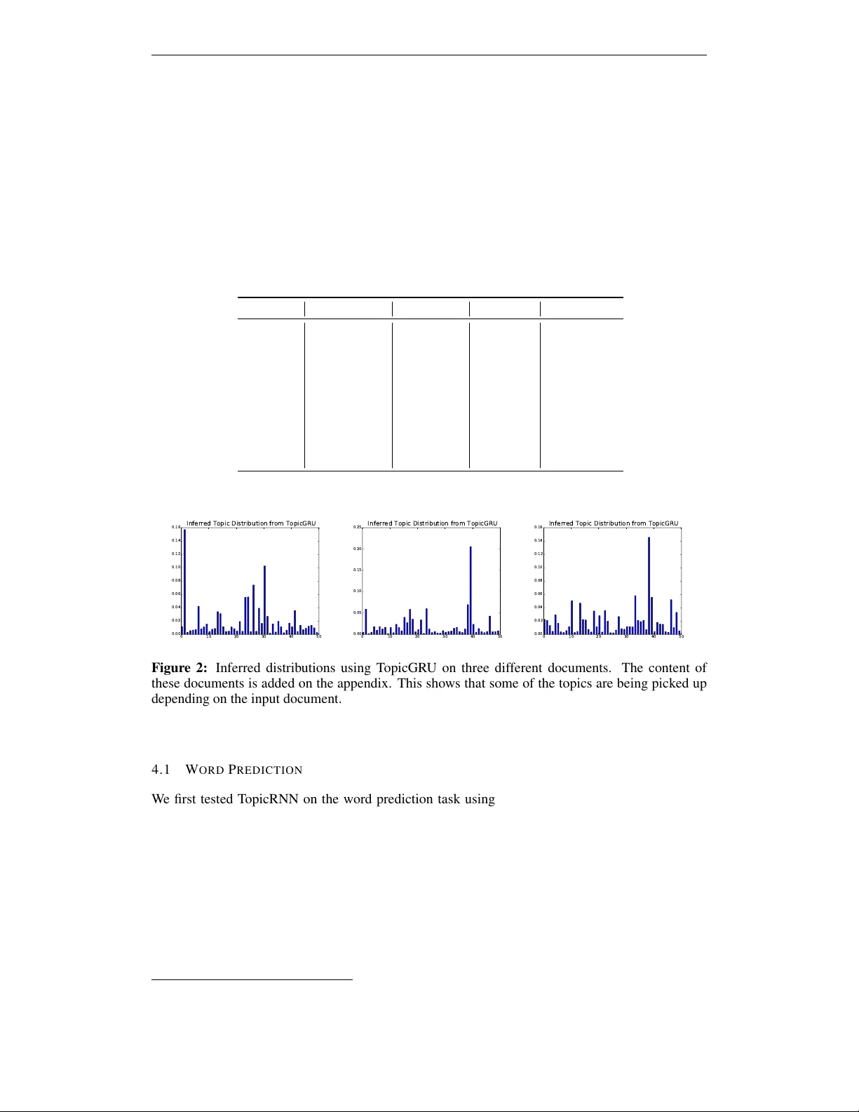
Published as a conference paper at ICLR 2017 T O P I C R N N : A R E C U R R E N T N E U R A L N E T W O R K W I T H L O N G - R A N G E S E M A N T I C D E P E N D E N C Y Adji B. Dieng ∗ Columbia Univ ersity abd2141@columbia.edu Chong W ang Deep Learning T echnology Center Microsoft Research chowang@microsoft.com Jianfeng Gao Deep Learning T echnology Center Microsoft Research jfgao@microsoft.com John Paisley Columbia Univ ersity jpaisley@columbia.edu A B S T R AC T In this paper , we propose T opicRNN, a recurrent neural network ( R N N )-based language model designed to directly capture the global semantic meaning relating words in a document via latent topics. Because of their sequential nature, R N N s are good at capturing the local structure of a word sequence – both semantic and syntactic – but might face dif ficulty remembering long-range dependencies. Intu- itiv ely , these long-range dependencies are of semantic nature. In contrast, latent topic models are able to capture the global semantic structure of a document but do not account for word ordering. The proposed T opicRNN model integrates the merits of R N N s and latent topic models: it captures local (syntactic) dependen- cies using an R N N and global (semantic) dependencies using latent topics. Unlike previous work on contextual R N N language modeling, our model is learned end- to-end. Empirical results on word prediction sho w that T opicRNN outperforms existing contextual R N N baselines. In addition, T opicRNN can be used as an un- supervised feature extractor for documents. W e do this for sentiment analysis on the IMDB movie revie w dataset and report an error rate of 6 . 28% . This is com- parable to the state-of-the-art 5 . 91% resulting from a semi-supervised approach. Finally , T opicRNN also yields sensible topics, making it a useful alternativ e to document models such as latent Dirichlet allocation. 1 I N T RO D U C T I O N When reading a document, short or long, humans hav e a mechanism that somehow allows them to remember the gist of what they ha ve read so far . Consider the following example: “ The U.S.pr esidential race isn’ t only drawing attention and contr oversy in the United States – it’ s being closely watched acr oss the globe. But what does the r est of the world think about a campaign that has already thr own up one surprise after another? CNN asked 10 journalists for their take on the race so far , and what their country might be hoping for in America ’ s next — ” The missing word in the text above is easily predicted by any human to be either Pr esident or Commander in Chief or their synon yms. There ha ve been v arious language models – from simple n - grams to the most recent R N N -based language models – that aim to solve this problem of predicting correctly the subsequent word in an observed sequence of w ords. A good language model should capture at least two important properties of natural language. The first one is correct syntax. In order to do prediction that enjoys this property , we often only need to consider a few preceding words. Therefore, correct syntax is more of a local property . W ord order matters in this case. The second property is the semantic coherence of the prediction. T o achieve ∗ W ork was done while at Microsoft Research. 1 Published as a conference paper at ICLR 2017 this, we often need to consider many preceding w ords to understand the global semantic meaning of the sentence or document. The ordering of the words usually matters much less in this case. Because they only consider a fixed-size context windo w of preceding words, traditional n -gram and neural probabilistic language models ( Bengio et al. , 2003 ) have difficulties in capturing global semantic information. T o overcome this, R N N -based language models ( Mikolov et al. , 2010 ; 2011 ) use hidden states to “remember” the history of a word sequence. Howe ver , none of these approaches explicitly model the two main properties of language mentioned abo ve, correct syntax and semantic coherence. Pre vious work by Chelba and Jelinek ( 2000 ) and Gao et al. ( 2004 ) exploit syntactic or semantic parsers to capture long-range dependencies in language. In this paper , we propose T opicRNN, a R N N -based language model that is designed to directly capture long-range semantic dependencies via latent topics. These topics provide context to the R N N . Contextual R N N s have recei ved a lot of attention ( Mikolov and Zweig , 2012 ; Mikolov et al. , 2014 ; Ji et al. , 2015 ; Lin et al. , 2015 ; Ji et al. , 2016 ; Ghosh et al. , 2016 ). Howe ver , the models closest to ours are the contextual R N N model proposed by Mikolov and Zweig ( 2012 ) and its most recent extension to the long-short term memory (LSTM) architecture ( Ghosh et al. , 2016 ). These models use pre-trained topic model features as an additional input to the hidden states and/or the output of the R N N . In contrast, T opicRNN does not require pre-trained topic model features and can be learned in an end-to-end fashion. W e introduce an automatic way for handling stop words that topic models usually hav e difficulty dealing with. Under a comparable model size set up, T opicRNN achiev es better perplexity scores than the contextual R N N model of Mikolov and Zweig ( 2012 ) on the Penn T reeBank dataset 1 . Moreover , T opicRNN can be used as an unsupervised feature extractor for do wnstream applications. For example, we deri ve document features of the IMDB mo vie re vie w dataset using T opicRNN for sentiment classification. W e reported an error rate of 6 . 28% . This is close to the state-of-the-art 5 . 91% ( Miyato et al. , 2016 ) despite that we do not use the labels and adversarial training in the feature e xtraction stage. The remainder of the paper is organized as follows: Section 2 provides background on R N N -based language models and probabilistic topic models. Section 3 describes the T opicRNN network ar - chitecture, its generativ e process and how to perform inference for it. Section 4 presents per-word perplexity results on the Penn T reeBank dataset and the classification error rate on the IMDB 100 K dataset. Finally , we conclude and provide future research directions in Section 5 . 2 BA C K G RO U N D W e present the background necessary for b uilding the T opicRNN model. W e first re view R N N -based language modeling, followed by a discussion on the construction of latent topic models. 2 . 1 R E C U R R E N T N E U R A L N E T W O R K - B A S E D L A N G U AG E M O D E L S Language modeling is fundamental to many applications. Examples include speech recognition and machine translation. A language model is a probability distrib ution over a sequence of words in a predefined vocabulary . More formally , let V be a vocab ulary set and y 1 , ..., y T a sequence of T words with each y t ∈ V . A language model measures the likelihood of a sequence through a joint probability distribution, p ( y 1 , ..., y T ) = p ( y 1 ) T Y t =2 p ( y t | y 1: t − 1 ) . T raditional n -gram and feed-forward neural network language models ( Bengio et al. , 2003 ) typically make Markov assumptions about the sequential dependencies between words, where the chain rule shown abo ve limits conditioning to a fix ed-size context windo w . R N N -based language models ( Mikolov et al. , 2011 ) sidestep this Markov assumption by defining the conditional probability of each word y t giv en all the previous words y 1: t − 1 through a hidden 1 Ghosh et al. ( 2016 ) did not publish results on the PTB and we did not find the code online. 2 Published as a conference paper at ICLR 2017 state h t (typically via a softmax function): p ( y t | y 1: t − 1 ) , p ( y t | h t ) , h t = f ( h t − 1 , x t ) . The function f ( · ) can either be a standard R N N cell or a more comple x cell such as GRU ( Cho et al. , 2014 ) or LSTM ( Hochreiter and Schmidhuber , 1997 ). The input and target words are related via the relation x t ≡ y t − 1 . These R N N -based language models hav e been quite successful ( Mikolov et al. , 2011 ; Chelba et al. , 2013 ; Jozefowicz et al. , 2016 ). While in principle R N N -based models can “remember” arbitrarily long histories if pro vided enough capacity , in practice such large-scale neural networks can easily encounter difficulties during opti- mization ( Bengio et al. , 1994 ; P ascanu et al. , 2013 ; Sutskev er , 2013 ) or o verfitting issues ( Sriv astava et al. , 2014 ). Finding better ways to model long-range dependencies in language modeling is there- fore an open research challenge. As motiv ated in the introduction, much of the long-range depen- dency in language comes from semantic coherence, not from syntactic structure which is more of a local phenomenon. Therefore, models that can capture long-range semantic dependencies in lan- guage are complementary to R N N s. In the following section, we describe a family of such models called probabilistic topic models. 2 . 2 P R O B A B I L I S T I C T O P I C M O D E L S Probabilistic topic models are a family of models that can be used to capture global semantic co- herency ( Blei and Lafferty , 2009 ). They provide a powerful tool for summarizing, organizing, and navigating document collections. One basic goal of such models is to find groups of words that tend to co-occur together in the same document. These groups of words are called topics and represent a probability distribution that puts most of its mass on this subset of the vocabulary . Documents are then represented as mixtures ov er these latent topics. Through posterior inference, the learned topics capture the semantic coherence of the words they cluster together ( Mimno et al. , 2011 ). The simplest topic model is latent Dirichlet allocation (LDA) ( Blei et al. , 2003 ). It assumes K underlying topics β = { β 1 , . . . , β K } , each of which is a distribution over a fixed vocab ulary . The generativ e process of LD A is as follows: First generate the K topics, β k ∼ iid Diric hlet( τ ) . Then for each document containing words y 1: T , independently generate document-lev el variables and data: 1. Draw a document-specific topic proportion vector θ ∼ Diric hlet( α ) . 2. For the t th word in the document, (a) Draw topic assignment z t ∼ Discrete( θ ) . (b) Draw word y t ∼ Discrete( β z t ) . Marginalizing each z t , we obtain the probability of y 1: T via a matrix factorization followed by an integration o ver the latent v ariable θ , p ( y 1: T | β ) = Z p ( θ ) T Y t =1 X z t p ( z t | θ ) p ( y t | z t , β )d θ = Z p ( θ ) T Y t =1 ( β θ ) y t d θ . (1) In LDA the prior distrib ution on the topic proportions is a Dirichlet distribution; it can be replaced by many other distributions. For example, the correlated topic model ( Blei and Lafferty , 2006 ) uses a log-normal distribution. Most topic models are “bag of words” models in that w ord order is ignored. This makes it easier for topic models to capture global semantic information. Howe ver , this is also one of the reasons why topic models do not perform well on general-purpose language modeling applications such as word prediction. While bi-gram topic models have been proposed ( W allach , 2006 ), higher order models quickly become intractable. Another issue encountered by topic models is that they do not model stop words well. This is because stop words usually do not carry semantic meaning; their appearance is mainly to make the sentence more readable according to the grammar of the language. The y also appear frequently in 3 Published as a conference paper at ICLR 2017 B B B B V V V V V V V V U U U U U U W W W W W (a) Xc (ba g- of -wor ds) stop wor ds e x cluded X (f ull docume nt) stop wor ds in clude d Y (ta r get docume nt) RNN U V B W (b) Figure 1: (a) The unrolled T opicRNN architecture: x 1 , ..., x 6 are words in the document, h t is the state of the R N N at time step t , x i ≡ y i − 1 , l 1 , ..., l 6 are stop word indicators, and θ is the latent representation of the input document and is unshaded by conv ention. (b) The T opicRNN model architecture in its compact form: l is a binary vector that indicates whether each word in the input document is a stop word or not. Here red indicates stop words and blue indicates content words. almost ev ery document and can co-occur with almost any word 2 . In practice, these stop words are chosen using tf-idf ( Blei and Lafferty , 2009 ). 3 T H E T O P I C R N N M O D E L W e next describe the proposed T opicRNN model. In T opicRNN, latent topic models are used to capture global semantic dependencies so that the R N N can focus its modeling capacity on the local dynamics of the sequences. W ith this joint modeling, we hope to achiev e better ov erall performance on downstream applications. The model. T opicRNN is a generati ve model. For a document containing the words y 1: T , 1. Draw a topic vector 3 θ ∼ N (0 , I ) . 2. Giv en word y 1: t − 1 , for the t th word y t in the document, (a) Compute hidden state h t = f W ( x t , h t − 1 ) , where we let x t , y t − 1 . (b) Draw stop word indicator l t ∼ Bernoulli( σ (Γ > h t )) , with σ the sigmoid function. (c) Draw word y t ∼ p ( y t | h t , θ , l t , B ) , where p ( y t = i | h t , θ , l t , B ) ∝ exp  v > i h t + (1 − l t ) b > i θ  . The stop word indicator l t controls how the topic vector θ af fects the output. If l t = 1 (indicating y t is a stop word), the topic vector θ has no contribution to the output. Otherwise, we add a bias to fa vor those words that are more lik ely to appear when mixing with θ , as measured by the dot product between θ and the latent word vector b i for the i th vocabulary word. As we can see, the long- range semantic information captured by θ directly affects the output through an additiv e procedure. Unlike Mikolov and Zweig ( 2012 ), the conte xtual information is not passed to the hidden layer of the R N N . The main reason behind our choice of using the topic vector as bias instead of passing it into the hidden states of the RNN is because it enables us to hav e a clear separation of the contributions of global semantics and those of local dynamics. The global semantics come from the topics which are meaningful when stop words are excluded. Howe ver these stop words are needed for the local dynamics of the language model. W e hence achieve this separation of global vs local via a binary decision model for the stop words. It is unclear ho w to achie ve this if we pass the topics to the 2 W allach et al. ( 2009 ) described using asymmetric priors to alleviate this issue. Although it is not clear how to use this idea in T opicRNN, we plan to in vestigate such priors in future work. 3 Instead of using the Dirichlet distribution, we choose the Gaussian distribution. This allows for more flexibility in the sequence prediction problem and also has adv antages during inference. 4 Published as a conference paper at ICLR 2017 hidden states of the RNN. This is because the hidden states of the RNN will account for all words (including stop words) whereas the topics exclude stop w ords. W e show the unrolled graphical representation of T opicRNN in Figure 1 (a). W e denote all model parameters as Θ = { Γ , V , B , W , W c } (see Appendix A.1 for more details). Parameter W c is for the inference network, which we will introduce below . The observations are the word sequences y 1: T and stop word indicators l 1: T . 4 The log marginal lik elihood of the sequence y 1: T is log p ( y 1: T , l 1: T | h t ) = log Z p ( θ ) T Y t =1 p ( y t | h t , l t , θ ) p ( l t | h t )d θ . (2) Model inference. Direct optimization of Equation 2 is intractable so we use variational inference for approximating this marginal ( Jordan et al. , 1999 ). Let q ( θ ) be the variational distrib ution on the marginalized variable θ . W e construct the variational objectiv e function, also called the evidence lower bound ( E L B O ), as follows: L ( y 1: T , l 1: T | q ( θ ) , Θ) , E q ( θ ) " T X t =1 log p ( y t | h t , l t , θ ) + log p ( l t | h t ) + log p ( θ ) − log q ( θ ) # ≤ log p ( y 1: T , l 1: T | h t , Θ) . Follo wing the proposed variational autoencoder technique, we choose the form of q ( θ ) to be an inference network using a feed-forward neural network ( Kingma and W elling , 2013 ; Miao et al. , 2015 ). Let X c ∈ N | V c | + be the term-frequency representation of y 1: T excluding stop words (with V c the vocab ulary size without the stop words). The v ariational autoencoder inference network q ( θ | X c , W c ) with parameter W c is a feed-forward neural network with ReLU activ ation units that projects X c into a K -dimensional latent space. Specifically , we have q ( θ | X c , W c ) = N ( θ ; µ ( X c ) , diag ( σ 2 ( X c ))) , µ ( X c ) = W 1 g ( X c ) + a 1 , log σ ( X c ) = W 2 g ( X c ) + a 2 , where g ( · ) denotes the feed-forward neural network. The weight matrices W 1 , W 2 and biases a 1 , a 2 are shared across documents. Each document has its o wn µ ( X c ) and σ ( X c ) resulting in a unique distribution q ( θ | X c ) for each document. The output of the inference network is a distribution on θ , which we regard as the summarization of the semantic information, similar to the topic proportions in latent topic models. W e show the role of the inference network in Figure 1 (b). During training, the parameters of the inference network and the model are jointly learned and updated via truncated backpropagation through time using the Adam algorithm ( Kingma and Ba , 2014 ). W e use stochastic samples from q ( θ | X c ) and the reparameterization trick to wards this end ( Kingma and W elling , 2013 ; Rezende et al. , 2014 ). Generating sequential text and computing perplexity . Suppose we are given a word sequence y 1: t − 1 , from which we have an initial estimation of q ( θ | X c ) . T o generate the next word y t , we compute the probability distribution of y t giv en y 1: t − 1 in an online fashion. W e choose θ to be a point estimate ˆ θ , the mean of its current distribution q ( θ | X c ) . Mar ginalizing over the stop word indicator l t which is unknown prior to observing y t , the approximate distribution of y t is p ( y t | y 1: t − 1 ) ≈ X l t p ( y t | h t , ˆ θ , l t ) p ( l t | h t ) . The predicted w ord y t is a sample from this predictiv e distribution. W e update q ( θ | X c ) by including y t to X c if y t is not a stop word. Howe ver , updating q ( θ | X c ) after each w ord prediction is expensi ve, so we use a sliding window as was done in Mikolov and Zweig ( 2012 ). T o compute the perplexity , we use the approximate predictiv e distribution abo ve. Model Complexity . T opicRNN has a complexity of O ( H × H + H × ( C + K ) + W c ) , where H is the size of the hidden layer of the R N N , C is the vocabulary size, K is the dimension of the topic vector , and W c is the number of parameters of the inference network. The contextual R N N of Mikolo v and Zweig ( 2012 ) accounts for O ( H × H + H × ( C + K )) , not including the pre-training process, which might require more parameters than the additional W c in our complexity . 4 Stop words can be determined using one of the sev eral lists available online. For example, http://www. lextek.com/manuals/onix/stopwords2.html 5 Published as a conference paper at ICLR 2017 4 E X P E R I M E N T S W e assess the performance of our proposed T opicRNN model on word prediction and sentiment analysis 5 . F or word prediction we use the Penn TreeBank dataset, a standard benchmark for as- sessing new language models ( Marcus et al. , 1993 ). For sentiment analysis we use the IMDB 100k dataset ( Maas et al. , 2011 ), also a common benchmark dataset for this application 6 . W e use R N N , LSTM, and GRU cells in our experiments leading to T opicRNN, T opicLSTM, and T opicGR U. T able 1: Five T opics from the T opicRNN Model with 100 Neurons and 50 T opics on the PTB Data. (The word s&p belo w shows as sp in the data.) Law Company Parties T rading Cars law spending democratic stock gm lawyers sales republicans s&p auto judge advertising gop price ford rights employees republican in vestor jaguar attorney state senate standard car court taxes oakland chairman cars general fiscal highway in vestors headquarters common appropriation democrats retirement british mr budget bill holders e xecuti ves insurance ad district merrill model 0 10 20 30 40 50 0.00 0.02 0.04 0.06 0.08 0.10 0.12 0.14 0.16 Inferred Topic Distribution from TopicGRU 0 10 20 30 40 50 0.00 0.05 0.10 0.15 0.20 0.25 Inferred Topic Distribution from TopicGRU 0 10 20 30 40 50 0.00 0.02 0.04 0.06 0.08 0.10 0.12 0.14 0.16 Inferred Topic Distribution from TopicGRU Figure 2: Inferred distributions using T opicGR U on three different documents. The content of these documents is added on the appendix. This shows that some of the topics are being picked up depending on the input document. 4 . 1 W O R D P R E D I C T I O N W e first tested T opicRNN on the word prediction task using the Penn Treebank (PTB) portion of the W all Street Journal. W e use the standard split, where sections 0-20 (930K tokens) are used for training, sections 21-22 (74K tokens) for validation, and sections 23-24 (82K tokens) for test- ing ( Mikolov et al. , 2010 ). W e use a vocab ulary of size 10 K that includes the special token unk for rare words and eos that indicates the end of a sentence. T opicRNN takes documents as inputs. W e split the PTB data into blocks of 10 sentences to constitute documents as done by ( Mikolov and Zweig , 2012 ). The inference network takes as input the bag-of-words representation of the input document. For that reason, the vocab ulary size of the inference network is reduced to 9551 after excluding 449 pre-defined stop words. In order to compare with previous work on contextual R N N s we trained T opicRNN using different network sizes. W e performed word prediction using a recurrent neural network with 10 neurons, 5 Our code will be made publicly av ailable for reproducibility . 6 These datasets are publicly av ailable at http://www.fit.vutbr.cz/~imikolov/rnnlm/ simple- examples.tgz and http://ai.stanford.edu/~amaas/data/sentiment/ . 6 Published as a conference paper at ICLR 2017 T able 2: T opicRNN and its counterparts exhibit lower perplexity scores across different network sizes than reported in Mikolo v and Zweig ( 2012 ). T able 2a shows per-word perplexity scores for 10 neurons. T able 2b and T able 2c correspond to per-w ord perplexity scores for 100 and 300 neurons respectiv ely . These results prove T opicRNN has more generalization capabilities: for example we only need a T opicGR U with 100 neurons to achie ve a better perplexity than stacking 2 LSTMs with 200 neurons each: 112.4 vs 115.9) (a) 10 Neurons V alid T est R N N (no features) 239 . 2 225 . 0 R N N (LD A features) 197 . 3 187 . 4 T opicRNN 184 . 5 172 . 2 T opicLSTM 188 . 0 175 . 0 T opicGR U 178 . 3 166.7 (b) 100 Neurons V alid T est R N N (no features) 150 . 1 142 . 1 R N N (LD A features) 132 . 3 126 . 4 T opicRNN 128 . 5 122 . 3 T opicLSTM 126 . 0 118 . 1 T opicGR U 118 . 3 112.4 (c) 300 Neurons V alid T est R N N (no features) − 124 . 7 R N N (LD A features) − 113 . 7 T opicRNN 118 . 3 112 . 2 T opicLSTM 104 . 1 99 . 5 T opicGR U 99 . 6 97.3 100 neurons and 300 neurons. For these experiments, we used a multilayer perceptron with 2 hidden layers and 200 hidden units per layer for the inference network. The number of topics was tuned depending on the size of the R N N . For 10 neurons we used 18 topics. For 100 and 300 neurons we found 50 topics to be optimal. W e used the validation set to tune the hyperparameters of the model. W e used a maximum of 15 epochs for the experiments and performed early stopping using the validation set. For comparison purposes we did not apply dropout and used 1 layer for the R N N and its counterparts in all the word prediction experiments as reported in T able 2 . One epoch for 10 neurons takes 2 . 5 minutes. For 100 neurons, one epoch is completed in less than 4 minutes. Finally , for 300 neurons one epoch takes less than 6 minutes. These experiments were ran on Microsoft Azure NC12 that has 12 cores, 2 T esla K80 GPUs, and 112 GB memory . First, we sho w fi ve randomly drawn topics in T able 1 . These results correspond to a network with 100 neurons. W e also illustrate some inferred topic distributions for several documents from T opicGR U in Figure 2 . Similar to standard topic models, these distributions are also relati vely peaky . Next, we compare the performance of T opicRNN to our baseline contextual R N N using perplexity . Perplexity can be thought of as a measure of surprise for a language model. It is defined as the exponential of the average negati ve log likelihood. T able 2 summarizes the results for dif ferent network sizes. W e learn three things from these tables. First, the perplexity is reduced the larger the network size. Second, R N N s with context features perform better than R N N s without context features. Third, we see that T opicRNN giv es lower perplexity than the previous baseline result reported by Mikolov and Zweig ( 2012 ). Note that to compute these perplexity scores for word prediction we use a sliding windo w to compute θ as we mo ve along the sequences. The topic vector θ that is used from the current batch of words is estimated from the previous batch of words. This enables fair comparison to pre viously reported results ( Mikolov and Zweig , 2012 ). 7 Another aspect of the T opicRNN model we studied is its capacity to generate coherent text. T o do this, we randomly drew a document from the test set and used this document as seed input to the inference network to compute θ . Our expectation is that the topics contained in this seed document are reflected in the generated text. T able 3 shows generated text from models learned on the PTB and IMDB datasets. See Appendix A.3 for more examples. 7 W e adjusted the scores in T able 2 from what was previously reported after correcting a bug in the compu- tation of the ELBO. 7 Published as a conference paper at ICLR 2017 T able 3: Generated text using the T opicRNN model on the PTB (top) and IMDB (bottom). the y believe that the y had senior damages to guarantee and frustration of unk stations eos the rush to minimum effect in composite trading the compound base inflated rate befor e the common charter ’ s report eos wells far go inc. unk of state contr ol funds without openly scheduling the university ’s exc hange rate has been downgraded it ’s unk said eos the united cancer & be gan critical increasing rate of N N at N N to N N ar e less for the country to trade r ate for mor e than three months $ N work ers wer e mixed eos lee is head to be watched unk month she eos but the acting surprisingly nothing is very good eos i cant believe that he can unk to a r ole eos may appear of for the stupid killer r eally to help with unk unk unk if you wan na go to it fell to the plot clearly eos it gets clear of this movie 70 are so bad me xico dir ection r egar ding those films eos then go as unk ’ s walk and after unk to see him try to unk befor e that unk with this film T able 4: Classification error rate on IMDB 100k dataset. T opicRNN provides the state of the art error rate on this dataset. Model Reported Error rate BoW (bnc) (Maas et al., 2011) 12 . 20% BoW ( b ∆ t ´ c) (Maas et al., 2011) 11 . 77% LD A (Maas et al., 2011) 32 . 58% Full + BoW (Maas et al., 2011) 11 . 67% Full + Unlabelled + BoW (Maas et al., 2011) 11 . 11% WRRBM (Dahl et al., 2012) 12 . 58% WRRBM + BoW (bnc) (Dahl et al., 2012) 10 . 77% MNB-uni (W ang & Manning, 2012) 16 . 45% MNB-bi (W ang & Manning, 2012) 13 . 41% SVM-uni (W ang & Manning, 2012) 13 . 05% SVM-bi (W ang & Manning, 2012) 10 . 84% NBSVM-uni (W ang & Manning, 2012) 11 . 71% seq2-bown-CNN (Johnson & Zhang, 2014) 14 . 70% NBSVM-bi (W ang & Manning, 2012) 8 . 78% Paragraph V ector (Le & Mikolov , 2014) 7 . 42% SA-LSTM with joint training (Dai & Le, 2015) 14 . 70% LSTM with tuning and dropout (Dai & Le, 2015) 13 . 50% LSTM initialized with word2vec embeddings (Dai & Le, 2015) 10 . 00% SA-LSTM with linear gain (Dai & Le, 2015) 9 . 17% LM-TM (Dai & Le, 2015) 7 . 64% SA-LSTM (Dai & Le, 2015) 7 . 24% V irtual Adversarial (Miyato et al. 2016) 5.91% T opicRNN 6.28% 4 . 2 S E N T I M E N T A N A LY S I S W e performed sentiment analysis using T opicRNN as a feature extractor on the IMDB 100K dataset. This data consists of 100,000 movie revie ws from the Internet Movie Database (IMDB) website. The data is split into 75% for training and 25% for testing. Among the 75K training revie ws, 50K are unlabelled and 25K are labelled as carrying either a positiv e or a negativ e sentiment. All 25K test revie ws are labelled. W e trained T opicRNN on 65K random training revie ws and used the remaining 10K revie ws for validation. T o learn a classifier , we passed the 25K labelled training re views through the learned T opicRNN model. W e then concatenated the output of the inference network and the last state of the R N N for each of these 25K revie ws to compute the feature vectors. W e then used these feature v ectors to train a neural network with one hidden layer , 50 hidden units, and a sigmoid activ ation function to predict sentiment, exactly as done in Le and Mikolov ( 2014 ). T o train the T opicRNN model, we used a vocabulary of size 5,000 and mapped all other words to the unk token. W e took out 439 stop words to create the input of the inference network. W e used 500 units and 2 layers for the inference network, and used 2 layers and 300 units per-layer for the 8 Published as a conference paper at ICLR 2017 Figure 3: Clusters of a sample of 10000 movie revie ws from the IMDB 100 K dataset using T op- icRNN as feature extractor . W e used K-Means to cluster the feature vectors. W e then used PCA to reduce the dimension to two for visualization purposes. red is a negati ve revie w and green is a positiv e revie w . R N N . W e chose a step size of 5 and defined 200 topics. W e did not use any regularization such as dropout. W e trained the model for 13 epochs and used the validation set to tune the hyperparameters of the model and track perplexity for early stopping. This experiment took close to 78 hours on a MacBook pro quad-core with 16GHz of RAM. See Appendix A.4 for the visualization of some of the topics learned from this data. T able 4 summarizes sentiment classification results from T opicRNN and other methods. Our error rate is 6 . 28% . 8 This is close to the state-of-the-art 5 . 91% ( Miyato et al. , 2016 ) despite that we do not use the labels and adversarial training in the feature extraction stage. Our approach is most similar to Le and Mikolov ( 2014 ), where the features were extracted in a unsupervised way and then a one-layer neural net was trained for classification. Figure 3 sho ws the ability of T opicRNN to cluster documents using the feature vectors as created during the sentiment analysis task. Revie ws with positiv e sentiment are coloured in green while revie ws carrying negati ve sentiment are shown in red. This sho ws that T opicRNN can be used as an unsupervised feature extractor for downstream applications. T able 3 shows generated text from models learned on the PTB and IMDB datasets. See Appendix A.3 for more examples. The overall generated text from IMDB encodes a ne gativ e sentiment. 5 D I S C U S S I O N A N D F U T U R E W O R K In this paper we introduced T opicRNN, a R N N -based language model that combines R N N s and latent topics to capture local (syntactic) and global (semantic) dependencies between words. The global dependencies as captured by the latent topics serve as contextual bias to an R N N -based lan- guage model. This contextual information is learned jointly with the R N N parameters by maxi- mizing the evidence lower bound of variational inference. T opicRNN yields competitiv e per-word perplexity on the Penn Treebank dataset compared to previous contextual R N N models. W e have reported a competitiv e classification error rate for sentiment analysis on the IMDB 100K dataset. W e have also illustrated the capacity of T opicRNN to generate sensible topics and text. In future work, we will study the performance of T opicRNN when stop words are dynamically discov ered during training. W e will also extend T opicRNN to other applications where capturing context is important such as in dialog modeling. If successful, this will allow us to ha ve a model that performs well across different natural language processing applications. R E F E R E N C E S Y . Bengio, P . Simard, and P . Frasconi. Learning long-term dependencies with gradient descent is difficult. IEEE transactions on neural networks , 5(2):157–166, 1994. Y . Bengio, R. Ducharme, P . V incent, and C. Jauvin. A neural probabilistic language model. journal of machine learning r esearc h , 3(Feb):1137–1155, 2003. 8 The experiments were solely based on T opicRNN. Experiments using T opicGRU/T opicLSTM are being carried out and will be added as an extended v ersion of this paper . 9 Published as a conference paper at ICLR 2017 D. Blei and J. Lafferty . Correlated topic models. Advances in neural information pr ocessing systems , 18:147, 2006. D. M. Blei and J. D. Lafferty . T opic models. T ext mining: classification, clustering, and applications , 10(71):34, 2009. D. M. Blei, A. Y . Ng, and M. I. Jordan. Latent dirichlet allocation. Journal of machine Learning r esear ch , 3(Jan):993–1022, 2003. C. Chelba and F . Jelinek. Structured language modeling. Computer Speech & Language , 14(4): 283–332, 2000. C. Chelba, T . Mikolov , M. Schuster , Q. Ge, T . Brants, P . K oehn, and T . Robinson. One bil- lion word benchmark for measuring progress in statistical language modeling. arXiv pr eprint arXiv:1312.3005 , 2013. K. Cho, B. V an Merriënboer , C. Gulcehre, D. Bahdanau, F . Bougares, H. Schwenk, and Y . Bengio. Learning phrase representations using rnn encoder-decoder for statistical machine translation. arXiv pr eprint arXiv:1406.1078 , 2014. J. Gao, J.-Y . Nie, G. W u, and G. Cao. Dependence language model for information retriev al. In Pr o- ceedings of the 27th annual international ACM SIGIR confer ence on Resear ch and development in information r etrieval , pages 170–177. A CM, 2004. S. Ghosh, O. V inyals, B. Strope, S. Roy , T . Dean, and L. Heck. Contextual lstm (clstm) models for large scale nlp tasks. arXiv pr eprint arXiv:1602.06291 , 2016. S. Hochreiter and J. Schmidhuber . Long short-term memory . Neural computation , 9(8):1735–1780, 1997. Y . Ji, T . Cohn, L. Kong, C. Dyer , and J. Eisenstein. Document context language models. arXiv pr eprint arXiv:1511.03962 , 2015. Y . Ji, G. Haffari, and J. Eisenstein. A latent variable recurrent neural network for discourse relation language models. arXiv preprint , 2016. M. I. Jordan, Z. Ghahramani, T . S. Jaakk ola, and L. K. Saul. An introduction to variational methods for graphical models. Machine learning , 37(2):183–233, 1999. R. Jozefowicz, O. V inyals, M. Schuster, N. Shazeer , and Y . W u. Exploring the limits of language modeling. arXiv preprint , 2016. D. Kingma and J. Ba. Adam: A method for stochastic optimization. arXiv pr eprint arXiv:1412.6980 , 2014. D. P . Kingma and M. W elling. Auto-encoding variational bayes. arXiv preprint , 2013. Q. V . Le and T . Mikolo v . Distrib uted representations of sentences and documents. In ICML , vol- ume 14, pages 1188–1196, 2014. R. Lin, S. Liu, M. Y ang, M. Li, M. Zhou, and S. Li. Hierarchical recurrent neural network for document modeling. In Pr oceedings of the 2015 Confer ence on Empirical Methods in Natural Language Pr ocessing , pages 899–907, 2015. A. L. Maas, R. E. Daly , P . T . Pham, D. Huang, A. Y . Ng, and C. Potts. Learning word vectors for sentiment analysis. In Pr oceedings of the 49th Annual Meeting of the Association for Compu- tational Linguistics: Human Language T echnologies-V olume 1 , pages 142–150. Association for Computational Linguistics, 2011. M. P . Marcus, M. A. Marcinkie wicz, and B. Santorini. Building a large annotated corpus of english: The penn treebank. Computational linguistics , 19(2):313–330, 1993. Y . Miao, L. Y u, and P . Blunsom. Neural variational inference for text processing. arXiv preprint arXiv:1511.06038 , 2015. T . Mikolov and G. Zweig. Context dependent recurrent neural network language model. In SLT , pages 234–239, 2012. 10 Published as a conference paper at ICLR 2017 T . Mikolo v , M. Karafiát, L. Burget, J. Cernock ` y, and S. Khudanpur . Recurrent neural netw ork based language model. In Interspeech , volume 2, page 3, 2010. T . Mikolov , S. K ombrink, L. Bur get, J. ˇ Cernock ` y, and S. Khudanpur . Extensions of recurrent neural network language model. In 2011 IEEE International Confer ence on Acoustics, Speec h and Signal Pr ocessing (ICASSP) , pages 5528–5531. IEEE, 2011. T . Mikolo v , A. Joulin, S. Chopra, M. Mathieu, and M. Ranzato. Learning longer memory in recurrent neural networks. arXiv pr eprint arXiv:1412.7753 , 2014. D. Mimno, H. M. W allach, E. T alley , M. Leenders, and A. McCallum. Optimizing semantic co- herence in topic models. In Pr oceedings of the Confer ence on Empirical Methods in Natural Language Pr ocessing , pages 262–272. Association for Computational Linguistics, 2011. T . Miyato, A. M. Dai, and I. Goodfellow . Adversarial training methods for semi-supervised text classification. stat , 1050:7, 2016. R. Pascanu, T . Mikolov , and Y . Bengio. On the difficulty of training recurrent neural networks. ICML (3) , 28:1310–1318, 2013. D. J. Rezende, S. Mohamed, and D. W ierstra. Stochastic backpropagation and approximate infer- ence in deep generativ e models. arXiv preprint , 2014. N. Sri vasta va, G. E. Hinton, A. Krizhe vsky , I. Sutske ver , and R. Salakhutdinov . Dropout: a simple way to prev ent neural networks from overfitting. Journal of Machine Learning Researc h , 15(1): 1929–1958, 2014. I. Sutske ver . T raining r ecurrent neur al networks . PhD thesis, Uni versity of T oronto, 2013. H. M. W allach. T opic modeling: beyond bag-of-words. In Pr oceedings of the 23rd international confer ence on Machine learning , pages 977–984. A CM, 2006. H. M. W allach, D. M. Mimno, and A. McCallum. Rethinking lda: Why priors matter . In Advances in neural information pr ocessing systems , pages 1973–1981, 2009. A A P P E N D I X A . 1 D I M E N S I O N O F T H E P A R A M E T E R S O F T H E M O D E L : W e use the follo wing notation: C is the vocab ulary size (including stop words), H is the number of hidden units of the R N N , K is the number of topics, and E is the dimension of the inference network hidden layer . T able 5 giv es the dimension of each of the parameters of the T opicRNN model (ignoring the biases). T able 5: Dimensions of the parameters of the model. U Γ W V B θ W 1 W 2 dimension C x H H H x H H x C K x C K E E A . 2 D O C U M E N T S U S E D T O I N F E R T H E D I S T R I B U T I O N S O N F I G U R E 2 Figure on the left: ’the’, ’market’, ’has’, ’gr own’, ’ r elatively’, ’quiet’, ’ since’, ’ the’, ’china’, ’crisis’, ’b ut’, ’if ’, ’ the’, ’japanese’, ’r eturn’, ’in’, ’force’, ’their’, ’financial’, ’might’, ’could’, ’compensate’, ’ to’, ’some’, ’extent’, ’for’, ’local’, ’in vestors’, "’", ’’, ’commitment’, ’another’, ’and’, ’critical’, ’factor’, ’is’, ’ the’, ’u.s. ’, ’hong’, ’kong’, "’ s", ’biggest’, ’export’, ’market’, ’even’, ’before’, ’the’, ’china’, ’crisis’, ’weak’, ’u.s. ’, ’demand’, ’was’, ’ slowing’, ’local’, ’economic’, ’gr owth’, ’’, ’ str ong’, ’consumer’, ’ spending’, ’in’, ’the’, ’u.s. ’, ’ two’, ’years’, ’ago’, ’helped’, ’’, ’the’, ’local’, ’economy’, ’at’, ’more’, ’ than’, ’twice’, ’its’, ’current’, ’r ate’, ’indeed’, ’a’, ’few’, ’economists’, ’maintain’, ’ that’, ’global’, ’forces’, ’will’, ’continue’, ’ to’, ’govern’, ’hong’, ’kong’, "’ s", ’economic’, ’’, ’once’, ’external’, ’conditions’, ’ such’, ’as’, 11 Published as a conference paper at ICLR 2017 ’u.s. ’, ’ demand’, ’swing’, ’in’, ’ the’, ’territory’, "’ s", ’favor’, ’ they’, ’ar gue’, ’local’, ’businessmen’, ’will’, ’pr obably’, ’over come’, ’their’, ’N’, ’worries’, ’and’, ’continue’, ’doing’, ’business’, ’as’, ’usual’, ’but’, ’economic’, ’ar guments’, ’however’, ’ solid’, ’wo’, "n’t", ’necessarily’, ’’, ’hong’, ’kong’, "’ s", ’N’, ’million’, ’people’, ’many’, ’are’, ’ refug ees’, ’having’, ’fled’, ’china’, "’ s", ’’, ’cycles’, ’of ’, ’political’, ’r epression’, ’and’, ’poverty’, ’ since’, ’the’, ’communist’, ’party’, ’took’, ’power’, ’in’, ’N’, ’as’, ’a’, ’r esult’, ’many’, ’of ’, ’ those’, ’now’, ’planning’, ’to’, ’leave’, ’hong’, ’kong’, ’ca’, "n’t", ’easily’, ’be’, ’’, ’by’, ’’, ’impr ovements’, ’in’, ’ the’, ’colony’, "’ s", ’political’, ’and’, ’economic’, ’climate’ Figure on the middle: ’it’, ’ said’, ’ the’, ’man’, ’whom’, ’it’, ’did’, ’not’, ’name’, ’had’, ’been’, ’found’, ’ to’, ’have’, ’the’, ’disease’, ’after’, ’hospital’, ’ tests’, ’once’, ’the’, ’disease’, ’was’, ’confirmed’, ’all’, ’ the’, ’man’, "’s", ’associates’, ’and’, ’family’, ’wer e’, ’ tested’, ’b ut’, ’none’, ’have’, ’ so’, ’far’, ’been’, ’found’, ’to’, ’have’, ’aids’, ’the’, ’newspaper’, ’ said’, ’ the’, ’man’, ’had’, ’for’, ’a’, ’long’, ’ time’, ’had’, ’a’, ’chaotic’, ’ sex’, ’life’, ’including’, ’r elations’, ’with’, ’for eign’, ’men’, ’ the’, ’newspaper’, ’said’, ’the’, ’polish’, ’government’, ’incr eased’, ’home’, ’electricity’, ’char ges’, ’by’, ’N’, ’N’, ’and’, ’doubled’, ’gas’, ’prices’, ’ the’, ’official’, ’news’, ’a gency’, ’’, ’ said’, ’ the’, ’incr eases’, ’wer e’, ’intended’, ’ to’, ’bring’, ’’, ’low’, ’ener gy’, ’char ges’, ’into’, ’line’, ’with’, ’pr oduction’, ’costs’, ’and’, ’compensate’, ’for’, ’a’, ’rise’, ’in’, ’coal’, ’prices’, ’in’, ’’, ’news’, ’ south’, ’kor ea’, ’in’, ’establishing’, ’ diplomatic’, ’ ties’, ’with’, ’poland’, ’yester day’, ’announced’, ’$’, ’N’, ’million’, ’in’, ’loans’, ’ to’, ’ the’, ’financially’, ’str apped’, ’warsaw’, ’government’, ’in’, ’a’, ’victory’, ’for’, ’en vir onmentalists’, ’hungary’, "’ s", ’parliament’, ’ terminated’, ’a’, ’multibillion-dollar’, ’river’, ’’, ’ dam’, ’being’, ’b uilt’, ’by’, ’’, ’firms’, ’ the’, ’’, ’ dam’, ’was’, ’designed’, ’ to’, ’be’, ’’, ’with’, ’another’, ’dam’, ’now’, ’nearly’, ’complete’, ’N’, ’miles’, ’’, ’in’, ’czechoslo vakia’, ’in’, ’ending’, ’hungary’, "’ s", ’part’, ’of ’, ’ the’, ’pr oject’, ’parliament’, ’authorized’, ’prime’, ’minister’, ’’, ’’, ’ to’, ’modify’, ’a’, ’N’, ’agreement’, ’with’, ’czechoslovakia’, ’which’, ’ still’, ’wants’, ’the’, ’dam’, ’ to’, ’be’, ’built’, ’mr . ’, ’’, ’said’, ’in’, ’parliament’, ’ that’, ’czechoslovakia’, ’and’, ’hungary’, ’would’, ’ suffer’, ’envir onmental’, ’damag e’, ’if ’, ’the’, ’’, ’’, ’wer e’, ’built’, ’as’, ’planned’ Figure on the right: ’in’, ’hartfor d’, ’conn. ’, ’the’, ’charter’, ’oak’, ’bridge’, ’will’, ’soon’, ’be’, ’ r eplaced’, ’ the’, ’’, ’’, ’fr om’, ’its’, ’’, ’’, ’to’, ’a’, ’park’, ’’, ’are’, ’possible’, ’citizens’, ’in’, ’peninsula’, ’ohio’, ’upset’, ’over’, ’changes’, ’ to’, ’a’, ’bridge’, ’ne gotiated’, ’a’, ’deal’, ’ the’, ’bottom’, ’half ’, ’of ’, ’ the’, ’’, ’will’, ’be’, ’ type’, ’f ’, ’while’, ’the’, ’ top’, ’half ’, ’will’, ’have’, ’the’, ’old’, ’bridge’, "’ s", ’’, ’pattern’, ’similarly’, ’highway’, ’engineers’, ’agr eed’, ’to’, ’keep’, ’ the’, ’old’, ’’, ’on’, ’ the’, ’key’, ’bridge’, ’in’, ’washington’, ’ d.c. ’, ’as’, ’long’, ’as’, ’ the y’, ’could’, ’install’, ’a’, ’crash’, ’barrier’, ’between’, ’ the’, ’ sidewalk’, ’and’, ’the’, ’ road’, ’’, ’’, ’ drink’, ’carrier’, ’competes’, ’with’, ’’, ’’, ’’, ’just’, ’got’, ’easier’, ’or’, ’ so’, ’claims’, ’’, ’corp. ’, ’the’, ’maker’, ’of ’, ’ the’, ’’, ’the’, ’chicago’, ’company’, "’ s", ’beverag e’, ’carrier’, ’meant’, ’ to’, ’r eplace’, ’’, ’’, ’at’, ’’, ’ stands’, ’and’, ’fast-food’, ’outlets’, ’r esembles’, ’ the’, ’plastic’, ’’, ’used’, ’on’, ’’, ’of ’, ’beer’, ’only’, ’ the’, ’’, ’hang’, ’fr om’, ’a’, ’’, ’of ’, ’’, ’ the’, ’new’, ’carrier’, ’can’, ’’, ’as’, ’many’, ’as’, ’four’, ’’, ’at’, ’once’, ’inventor’, ’’, ’marvin’, ’ says’, ’his’, ’design’, ’virtually’, ’’, ’’ A . 3 M O R E G E N E R AT E D T E X T F R O M T H E M O D E L : W e illustrate below some generated text resulting from training T opicRNN on the PTB dataset. Here we used 50 neurons and 100 topics: T ext1: b ut the refcorp bond fund might have been unk and unk of the point rate eos house in national unk wall restr aint in the pr operty pension fund sold willing to zenith was guaranteed by $ N million at short-term rates maturities ar ound unk pr oducts eos deposit posted yields slightly T ext2: it had happened by the treasury ’s clinical fund month wer e under national disap- pear institutions but secr etary nicholas instruments succeed eos and in vestors age far compound 12 Published as a conference paper at ICLR 2017 averag e new york stock exchang e bonds typically sold $ N shar es in the N but paying yields further an averag e rate of long-term funds W e illustrate below some generated text resulting from training T opicRNN on the IMDB dataset. The settings are the same as for the sentiment analysis experiment: the film ’ s gr eatest unk unk and it will likely very nice movies to go to unk why various david pro ves eos the story wer e always well scary friend high can be a very strange unk unk is in love with it lacks even perfect for unk for some of the worst movies come on a unk gave a r ock unk eos whatever let ’s possible eos that kyle can ’t differ ent reasons about the unk and was not what you ’r e not a fan of unk unk us r ock whic h unk still in unk ’ s music unk one as A . 4 T O P I C S F R O M I M D B : Below we show some topics resulting from the sentiment analysis on the IMDB dataset. The total number of topics is 200 . Note here all the topics turn around movies which is expected since all revie ws are about movies. T able 6: Some T opics from the T opicRNN Model on the IMDB Data. pitt tarantino producing k en hudson campbell campbell cameron dramas popcorn opera dragged africa spots vicious cards practice carrey robinson circumstances dollar francisco unbearable ninja kong flight burton cage los catches cruise hills awake kubrick freeman re volution nonsensical intimate useless rolled friday murphy refuses cringe costs lie easier expression 2002 cheese lynch alongside repeated kurosaw a struck scorcese 13