Combinatorics of Distance Covariance: Inclusion-Minimal Maximizers of Quasi-Concave Set Functions for Diverse Variable Selection
In this paper we show that the negative sample distance covariance function is a quasi-concave set function of samples of random variables that are not statistically independent. We use these properties to propose greedy algorithms to combinatorially…
Authors: Praneeth Vepakomma, Yulia Kempner
Com binatorics of Distance Co v ariance: Inclusion-Minimal Maximizers of Quasi-Conca v e Set F unctions for Div erse V ariable Selection Praneeth V epak omma a,b, ∗ , Y ulia Kempner c a R utgers University b Motor ola Solutions c Holon Institute of T e chnolo gy Abstract In this paper w e sho w that the negativ e sample distance cov ariance function is a quasi- conca ve set function of samples of random v ariables that are not statistically indep enden t. W e use these prop erties to prop ose greedy algorithms to combinatorially optimize some di- v ersity (lo w statistical dependence) promoting functions of distance co v ariance. Our greedy algorithm obtains all the inclusion-minimal maximizers of this div ersity promoting ob jective. Inclusion-minimal maximizers are m ultiple solution sets of globally optimal maximizers that are not a prop er subset of any other maximizing set in the solution set. W e present results up on applying this approach to obtain diverse features (co v ariates/v ariables/predictors) in a feature selection setting for regression (or classification) problems. W e also com bine our div erse feature selection algorithm with a distance cov ariance based relev an t feature selec- tion algorithm of [ 7 ] to pro duce subsets of cov ariates that are b oth relev an t y et ordered in non-increasing lev els of diversit y of these subsets. Keywor ds: Distance co v ariance, quasi-conca v e set function, minimal-maximizers, regression, div erse feature selection, greedy algorithm, combinatorics. 1. In tro duction 1.1. The classic al pr oblem of variable sel e ction: The problem of "v ariable selection" also known as "feature selection" or "cov ariate se- lection" is a prominent problem in statistics and machine learning. The goal in here is to b e able to choose an optimal subset of cov ariates in a regression or classification setting that w ould p erform optimally with resp ect to the out-of-sample prediction or classification accu- racy when the chosen subset is used to predict (or classify) one or more real-v alued resp onse ∗ corresp onding author Email addr esses: praneeth@scarletmail.rutgers.edu (Praneeth V epakomma), yuliak@hit.ac.il (Y ulia Kempner) Pr eprint submitte d to arXiv 2017-02-20 v ariables (in regression) or one or more categorical v ariables (in classification). There ha v e b een an umpteen num b er of techniques developed for this problem under a broadly v arying sp ectrum of assumptions. 1.2. The mor e r e c ent pr oblem of diverse variable sele ction: T raditional feature selection algorithms hav e the primary goal of finding the b est feature subset that is relev ant to a regression or classification task. More recen tly , there has been a strong fo cus on not just the ab ov e mentioned goal of relev an t feature selection but also on selecting a "small" subset of "diverse" features. Div ersit y is useful for several reasons such as interpretabilit y , robustn ess to noise and in some cases to cater to reduction of real-life costs of costly feature acquisition for guiding feature engineering to decide on what other features could b e acquired etc. 1.2.1. Some existing work on diversific ation: The authors in [ 2 ] provide a solution in the sp ecific case of linear regression through a form ulation where a div ersity promoting sub-mo dular regularizer is added to the standard linear regression problem. In this setting the solution is obtained by greedy algorithms that optimize a submo dular function based ob jective. Although this is an interesting approach, w e’d like to p oin t that this approac h restricts the regression mo del to b e linear unlike it b eing generalized to an y regression (non-linear and linear) mo dels. Another imp ortan t issue with this approac h is that their solution is not globally optimal but is instead an approximation with a w ell-known (in submo dular optimization) 1 − 1 e st yled guarantee of (1 − e − b.γ ( U,k ) ) .OP T c , where O P T is the optimal solution, γ ( U, k ) is a function of the solution subset of features U obtained through their algorithm and it’s cardinalit y k (i.e., the num b er of features in U ). b, c are algorithm dep endent constan ts dep ending on the sp ecific c hoice of algorithm out of m ultiple algorithms that they prop ose. Note that (1 − 1 e ) is appro ximately equal to 63% . 1.2.2. Existing work on diversific ation with mutual-information: Another p opular approac h is [ 1 ] which is based on measuring div ersit y and relev ancy through functions of mutual-information. Their solution appro ximately optimizes their pro- p osed ob jective as obtaining a global solution w ould require O ( n | S | ) searc h op erations where n is the num b er of samples and | S | is the cardinality of the n umber of features required to b e selected b y the algorithm. This can b e a prohibitively large num b er in the case of many practical datasets and required | S | . 1.3. A dvantages of our pr op ose d algorithms: The tec hnique prop osed in b elo w sections of our pap er has tw o ma jor adv an tages: 1. Our solution to our prop osed diversit y encouraging ob jective function is globally opti- mal with no approximation error unlik e the 1 − 1 e st yled appro ximate solution provided b y [ 2 ] or the unquantified appro ximation error pro vided by [ 1 ]. W e also prop ose an approac h that is completely devoid of any parameters and provide a global solution to our prop osed form ulation. That said, w e do completely recognize that the ob jectiv e 2 function prop osed in our technique v aries from the ob jectiv e functions prop osed in existing tec hniques. 2. Another adv an tage of our approach is that it is indep endent of the choice of regression (linear/non-linear) or classification (linear/non-linear) mo del to b e used unlike the w ork by [ 2 ] which focusses only on linear regression. 3. Our approach can directly b e used for div ersified feature selection in b oth cases of univ ariate or m ultiv ariate (vector-v alued) resp onses (in regression) or m ulti-lab el (in classification) without mo difying our prop osed ob jectiv e function or algorithm while the approach in [ 2 ] do es not seem to extend trivially b ey ond the univ ariate resp onse case in linear regression without mo difying their regularized ob jective function or al- gorithmic routines. Prior to getting in to the crux of our prop osed theoretical results and algorithmic im- plications, w e’d lik e to note that in theory our approac h can b e explicitly parametrized by a trade-off parameter to control the trade-off b et ween relev ancy and div ersit y of features selected. Suc h tuning of trade-offs is not the main fo cus of this pap er. The previously pro- p osed approac h using sp ectral regularization [ 2 ] do es parametrize this through regularization parameters that w eigh the submo dular regularizer appropriately . 2. Problem F ormulation: In this pap er we cov er the follo wing three problems: Problem I: Div erse F eature Selection The goal here is to find a subset of features that ha ve the least statistical dep endence amongst eac h other. This implies that the selected features w ould b e div erse. Problem I I: All-Relev ant F eature Selection The goal here is to find a subset of features that are most statistically dep en- den t on a resp onse v ariable. Problem I I I: Diverse and Relev ant F eature Selection The goal here is to find a subset of features that are more statistically d e- p enden t on a resp onse v ariable while also being less statistically dep enden t amongst eac h other. W e presen t a greedy-algorithm with exactly optimal solutions in this pap er for our formu- lated ob jective to solv e Problem I. W e p oin t to an existing approac h for Problem I I and prop ose simple metho dologies for Problem I I I where the metho dologies are based on solu- tions of Problem I and I I. Before w e get to the main result of our pap er, our suggested t w o simple metho dological approaches for Problem I I I are: 3 (a.) Con trolled approac h: In this approach, we first choose a subset of features that "indi- vidually" hav e a statistical dep endency i.e ≥ α ∈ R + with resp onse v ariable and call this subset the controlled set. W e then run our algorithm prop osed for Problem I for c ho osing a diverse set of features from this con trolled set. (b.) T w o-stage approac h: In this approach, the Problem I I I could b e approac hed by solving Problem I I follow ed b y Problem I or vice-v ersa. 2.1. Main R esult of the p ap er: So to clearly reiterate, our main and most nov el contribution of this pap er is our pro- p osed algorithm for Problem I. 3. Preliminaries: In this section w e in tro duce some preliminaries ab out distance correlation and distance co v ariance whic h w e extensively use in our pap er to build up to wards our prop osed theoretical results. 3.1. Distanc e Covarianc e and Distanc e Corr elation: Distance Correlation [ 3 ] is a measure of nonlinear statistical dep endencies b et ween ran- dom v ectors of arbitrary dimensions. W e describ e b elow distance cov ariance ν 2 ( x , y ) b etw een random v ariables x ∈ R d and y ∈ R m with finite first momen ts is a non-negative num b er as ν 2 ( x , y ) = Z R d + m | f x , y ( t, s ) − f x ( t ) f y ( s ) | 2 w ( t, s ) dtds (1) where w ( t, s ) is a weigh t function as defined in [ 3 ], f x , f y are characteristic functions of x , y and f x , y is the join t characteristic function. The distance cov ariance is zero if and only if random v ariables x and y are indep en- den t. Using the ab o ve definition of distance cov ariance, w e hav e the follo wing expression for Distance Correlation from [ 3 ]: The squared Distance Correlation b etw een random v ariables x ∈ R d and y ∈ R m with finite first momen ts is a nonnegative num b er is defined as ρ 2 ( x , y ) = ( ν 2 ( x , y ) √ ν 2 ( x , x ) ν 2 ( y , y ) , ν 2 ( x , x ) ν 2 ( y , y ) > 0 . 0 , ν 2 ( x , x ) ν 2 ( y , y ) = 0 . (2) The Distance Correlation defined ab ov e has the follo wing in teresting prop erties; 1. ρ 2 ( x , y ) is applicable for arbitrary dimensions d and m of x and y resp ectiv ely . 2. ρ 2 ( x , y ) = 0 if and only if x and y are indep endent. 3. ρ 2 ( x , y ) satisfies the relation 0 ≤ ρ 2 ( x , y ) ≤ 1 . 4 3.2. Sample Distanc e Covarianc e and Sample Distanc e Corr elation: W e provide the definition of sample v ersion of distance co v ariance [ 3 ] giv en samples { ( x k , y k ) | k = 1 , 2 , . . . , n } sampled i.i.d. from joint distribution of random vectors x ∈ R d and y ∈ R m . T o do so, we define t wo squared Euclidean distance matrices E X and E Y , where each en try [ E X ] k,l = k x k − x l k 2 and [ E Y ] k,l = k y k − y l k 2 with k , l ∈ { 1 , 2 , . . . , n } . These squared distance matrices are then double-cen tered b y making their row and column sums zero and are denoted as b E X , b Q X , resp ectively . So given a double-cen tering matrix J = I − 1 n 11 T , w e ha ve b E X = JE X J and b E Y = JE Y J . The sample distance co v ariance and sample distance correlation can no w b e defined as follows: Definition 3.1. Sample Distance Co v ariance [ 3 ]: Giv en i.i.d samples X ×Y = { ( x k , y k ) | k = 1 , 2 , 3 , . . . , n } and corresp onding double centered Euclidean distance matrices b E X and b E Y , then the squared sample distance correlation is defined as, ˆ ν 2 ( X , Y ) = 1 n 2 n X k,l =1 [ b E X ] k,l [ b E Y ] k,l , Using this, sample distance correlation is giv en by ˆ ρ 2 ( X , Y ) = ( ˆ ν 2 ( X , Y ) √ ˆ ν 2 ( X , X ) ˆ ν 2 ( Y , Y ) , ˆ ν 2 ( X , X ) ˆ ν 2 ( Y , Y ) > 0 . 0 , ˆ ν 2 ( X , X ) ˆ ν 2 ( Y , Y ) = 0 . 4. K osorok’s Distance Co v ariance Indep endence Inequalit y: If X , Z ∈ R p and Y ∈ R q and if and only if Z | = ( X , Y ) then ν 2 ( X + Z , Y ) ≤ ν 2 ( X , Y ) (3) Note that | = indicates ’statistically indep enden t’ in statistical literature. This implies that for eac h X , Y , Z that are not pairwise statistically independent (i.e distance co v ariance b et ween components of an y subset of cardinalit y 2 of X , Y , Z is p ositiv e) then ν 2 ( X + Z , Y ) > ν 2 ( X , Y ) (4) 5. Pro of of K osorok’s Distance Co v ariance Inequality The K osorok’s Distance Co v ariance Indep endence Inequalit y was pro ved in [ 7 , 5 ] and is based on the prop erty of characteristic functions (denoted b elo w by f ) that | f X + Z , Y ( t, s ) − f X + Z ( t ) f Y ( s ) | 2 ≤ | f Z ( t ) | 2 | f X , Y ( t, s ) − f X ( t ) f Y ( s ) | 2 (5) and | f Z ( t ) | 2 ≤ 1 . The equation ( 5 ) abov e can b e obtained by these facts | f X + Z , Y ( t, s ) − f X + Z ( t ) f Y ( s ) | 2 = | E e it T ( X + Z )+ is T Y − E e it T ( X + Z ) E e is T Y | 2 (6) = | E e it T X + is T Y E e it T Z − E e it T X E e it T Z E e it T Y | 2 = | f X , Y ( t, s ) f Z ( t ) − f X ( t ) f Z ( t ) f Y ( s ) | 2 = | f Z ( t ) | 2 | f X , Y ( t, s ) − f X ( t ) f Y ( s ) | 2 5 whic h with implication from | f Z ( t ) | 2 ≤ 1 gives ν 2 ( X + Z , Y ) ≤ ν 2 ( X , Y ) (7) W e kno w that if E | X | d < ∞ , E | X + Z | m < ∞ and E | Y | d < ∞ , then from [ 3 ] lim n →∞ ν 2 n ( X + Z , Y ) = ν 2 ( X + Z , Y ) and lim n →∞ ν 2 n ( X , Y ) = ν 2 ( X , Y ) Th us, for the sample distance cov ariance, if n is large enough, we should hav e V 2 n ( X + Z , Y ) ≤ V 2 ( X , Y ) only under the assumption of indep endence b etw een ( X , Y ) and Z . Note that ν n indicates sample distance co v ariance and ν indicates p opulation distance cov ariance. Note: In the case where considering ( X ∪ Z ) is of interest, we could use the ab o ve theorem b y incorp orating degenerated random v ectors as follows: Supp ose X ∈ R p 1 and Z ∈ R p 2 , then we augmen t X and Z to b e ˜ X = ( X , 0 p 2 ) and ˜ Z = ( 0 p 1 , Z ) resp ectively . ˜ X and ˜ Z are therefore of the same dimension and ˜ X + ˜ Z = ( X , Z ) . Therefore the X ∪ Z op eration in the con text of computing ˆ ν ( X ∪ Z , Y ) with matrices X , Z , Y is equiv alent to app ending the columns of X with the columns of Z follo wed by computing the sample-distan ce co v ariance b et ween the resulting matrix and Y . 6. Quasi-Conca v e Set F unctions 6.1. Notation and definitions: W e now describ e some notation and in tro duce some definitions that w e use through out the paper in the sections b elow. W e use b old faced X to denote the complete ground set of features/co v ariates and indexed X i to denote the i ’th cov ariate. That is we use i indexed subsets lik e S i to indicate a singleton (unit cardinality) elemen t of S lab eled by i . W e denote the resp onse v ariable in a regression setting with Y . W e denote the set 2 X \ { φ, X } b y P − X and use \ to denote set difference, i.e X \ Z = { x : x ∈ X and x 6∈ Z } . Giv en a set system ( X , F ) which is a collection F of subsets of a ground set X where F ⊆ 2 X , w e define a quasi-concav e set function as giv en b elow. Definition 6.1 ( Quasi-Conca ve Set F unction [ 4 ],[ 9 ]: ) . A function F : F 7→ R defined on a set system ( X , F ) is quasi-conca v e if for each S , T ∈ F , F ( S ∩ T ) ≥ min { F ( S ) , F ( T ) } (8) Definition 6.2 ( Monotone Link age F unction [ 9 ]: ) . A function π ( X i , Z ) defined on Z ∈ P − X , X i ∈ X \ Z is called a monotone link age function if π ( X i , S ) ≥ π ( X i , T ) , S ⊆ T ∈ F , ∀ X i ∈ X \ T (9) W e’d lik e to note for the clarity of the reader that X i is an element while S , T are sets. Therefore, to mak e this distinction clear we denote sets in b old-faced fon t and elements otherwise. 6 7. Some Com binatorial Prop erties of Negativ e Distance Co v ariance W e now prov e some quasi-concav e as w ell as monotone link age set function prop erties of some functions of negativ e distance cov ariance. Theorem 7.1 (Quasi-Conca ve Distance Co v ariance Set F unction Theorem) . If we have S ∩ T 6 = ∅ and ∀ S , T , Y if ν 2 ( S , T ) > 0 ∧ ν 2 ( S , Y ) > 0 ∧ ν 2 ( T , Y ) > 0 then we have − ν 2 ( S ∩ T , Y ) ≥ min ( − ν 2 ( S , Y ) , − ν 2 ( T , Y )) (10) Pr o of. If S ∩ T = S then since S ⊆ T the K osorok’s distance cov ariance inequalit y implies − ν 2 ( S , Y ) ≥ − ν 2 ( T , Y ) (11) Therefore w e hav e − ν 2 ( S ∩ T , Y ) ≥ min ( − ν 2 ( S , Y ) , − ν 2 ( T , Y )) Similarly , if S ∩ T = T , then since T ⊆ S − ν 2 ( T , Y ) ≥ − ν 2 ( S , Y ) (12) and therefore − ν 2 ( S ∩ T , Y ) ≥ min ( − ν 2 ( S , Y ) , − ν 2 ( T , Y )) (13) In the cases of S ∩ T ⊂ S and S ∩ T ⊂ T the K osorok’s distance cov ariance inequality implies − ν 2 ( S ∩ T , Y ) > − ν 2 ( S , Y ) (14) and − ν 2 ( S ∩ T , Y ) > − ν 2 ( T , Y ) (15) So − ν 2 ( S ∩ T , Y ) ≥ min ( − ν 2 ( S , Y ) , − ν 2 ( T , Y )) (16) 7.1. A monotone linkage function of distanc e c ovarianc e: Lemma 7.2. The function π ( X i , S ) of distanc e c ovarianc e define d on X i / ∈ S as π ( X i , S ) X i / ∈ S = X S j ∈ S − ν 2 ( X i , S j ) (17) is a monotone linkage function 7 Pr o of: F or S ⊆ T w e hav e π ( X i , T ) X i / ∈ T = X S j ∈ S − ν 2 i ( X i , S j ) − X T j ∈ T \ S ν 2 i ( X i , T j ) ≤ π ( X i , S ) X i / ∈ T = X S j ∈ S − ν 2 i ( X i , S j ) (18) W e would also lik e to note that as ν ( · ) is a non-negative function the ab ov e inequalit y do es hold true. Theorem 7.3. [ 4 ] The function M π ( T ) = min X i ∈ X \ T π ( X i , T ) is a quasi-c onc ave set function. Pr o of: The pro of is in the pro of of Assertion 1 in [ 4 ] 8. Div erse F eature Selection: W e aim to find all the subsets that maximize the function M π ( T ) which result in the solutions whic h for diverse features. arg max T ⊂ X M π ( T ) (19) The ab o ve equation ( 19 ) can be written as arg max T ⊂ X min X i ∈ X \ T π ( X i , T ) (20) This problem do es not necessarily ha ve a single, unique solution and hence w e aim to find all the subsets that are maximizers of ( 20 ). These are essen tially subsets that are each maximally separated from their corresp onding nearest neigh b or where the notion of nearness to their neigh b or is given b y ( 17 ). Definition 8.1 ( π -series: ) . W e refer to a series s π = ( X i 1 , . . . , X i N ) as a π -series if π ( X i k +1 , S k ) = min X i ∈ X \ S k π ( X i , S k ) (21) for an y starting set S k = { X i 1 , . . . , X i k } , k = 1 , . . . , N − 1 . Therefore it is a wa y of greedily p opulating a series that can start with an y first element X i 1 b eing the current series, but the subsequen t element to b e added to the series, m ust b e the elemen t that minimizes the element to current series function of π ( X i k + 1 , S k ) where X i k + 1 is the next elemen t added and S k is the curren t series. Definition 8.2 ( π -cluster ) . A subset S ∈ P − X will b e referred to as a π -cluster if there exists a π -series, s π = ( X i 1 , . . . , X i N ) , suc h that S is a maximizer of M π ( S k ) ov er all starting sets S k of s π . 8 Theorem 8.1. [ 4 ] If for a π -series s π = ( X i 1 , X i 2 , . . . , i N ) , a subset S ⊂ X c ontains X i 1 , and if X i k +1 is the first element in s π not c ontaine d in S (for some k ∈ { 1 , . . . , N − 1 } , then M π ( S k ) ≥ M π ( S ) (22) wher e S k = ( X i 1 , . . . , X i k ) . In p articular, if S is an inclusion-minimal maximizer of M π (with r e gar d to P − X ) , then S = S k , that is, S is a π -cluster. Pr o of. M π ( S k ) = π ( X i k +1 , S k ) by definition. Since S k ⊆ S w e hav e π ( X i k +1 , S k ) ≥ π ( X i k + 1 , S ) b y monotonicit y . T o end the proof, note that π ( X i k +1 , S ) ≥ M π ( S ) because M π ( S ) = min X i ∈ X \ Z π ( X i , S ) and X i k +1 / ∈ S Prop osition 8.2. [ 4 ] If S 1 , S 2 ⊂ X ar e overlapping maximizers of a quasi-c onc ave set function M π ( S ) over P − X , then S 1 ∩ S 2 is also a maximizer of M π ( S ) . Pr o of. It directly follo ws from ( 8 ). This implies that the minimal maximizers of a quasi-conv ex set function are not ov er- lapping. Moreo ver, any nonminimal maximizer can b e uniquely partitioned into a set of the minimal ones. Theorem 8.3. Each maximizer of a quasi-c onc ave set function on P − X is a union of its inclusion-minimal maximizers. Pr o of. Indeed, if S ∗ is a maximizer of M π ( S ) ov er P − X , then, according to Theorem 8.1 , for an y X i ∈ S ∗ , there exists a minimal maximizer included in S ∗ and con taining X i . 9 8.1. Our gr e e dy algorithm for diverse variable sele ction with distanc e c ovarianc e for solving Pr oblem I : Algorithm 1 DiverseMinimalMaximDCoV: Div erse Com binatorial Distance Cov ariance 1: function =DiverseMinimalMaximDCoV ( X ) 2: for all X i ∈ X do 3: Greedily form π -series s π ( x ) = ( X i , X i 2 . . . X i N ) starting from X i as its first elemen t. 4: for eac h π -series s π ( x ) in step 3 do 5: Find a corresp onding smallest starting subset T x with M π ( T x ) = max 1 ≤ k ≤ N − 1 π ( X i k + 1 , { X i 1 , . . . , X i k } ) 6: end for 7: end for 8: Among the non-coinciding minimal π -clusters T x ’s c ho ose those that maximize M π ( T x ) = min X i ∈ X \ T x π ( X i , T x ) all of whic h are the required minimal maximizers, and we return them as minimalMax 9: return (minimalMax) 10: end function The ab ov e algorithm finds all minimal maximizers i n O ( N 3 g ) time where g is the a v- erage time required to compute the v alue of π ( X i , S ) for any X i , S . The fastest v ersion of computing distance co v ariance to date is O ( N log N ) and prop osed in [ 6 ]. Theorem 8.4. The algorithm ab ove finds al l the minimal maximizers over P − X . Pr o of. F rom Theorem 8.1 it follo ws that eac h elemen t of minimalMax is a maximizer of M π ( S ) ov er P − X . Assume that there is a minimal maximizer S that do es not b elong to minimalMax, and let X i ∈ S . Then, according to Theorem 8.1 , there exist π -series starting from X i and minimal π -cluster T x ⊆ S con taining X i with M π ( T x ) ≥ M π ( S ) . Since S do es not b elong to minimalMax, and, according to steps 5 and 8 of the algorithm, T x or some subset of T x b elongs to minimalMax, there are a minimal maximizer strictly included in S whic h contradicts the minimality of S . Putting all these results together w e present our algorithm in Algorithm 1 ab o ve. 9. All-Relev ant F eature Selection In addition to our algorithm prop osed ab ov e, w e would lik e to p oint to a recent algorithm prop osed in [ 7 ] for the purp ose of solving Problem II using distance cov ariance. W e presen t this algorithm in Algorithm 2 b elow. 10 Algorithm 2 Kong-W ang-W ahba’s All-Relev ant F eature Selection algorithm for Problem I I: 1: function K ong-W ang-W ahba ’s Algorithm ( X ) 2: Calculate marginal sample distance correlations ρ n ( X i , Y ) for v ariables X i for i = 1 , . . . , n with the resp onse Y . 3: Rank the v ariables in decreasing order of the sample distance correlations. Denote the ordered v ariables as x 1 , x 1 , . . . , x n . Start with X s = { x 1 } . 4: for all i from 2 to n do Keep adding x i to X s if ν n ( X s Y ) , the sample distance cov ariance, do es not decrease. Stop otherwise. 5: end for return ( X s ) 6: end function 10. Div erse and Relev ant F eature Selection A metho dological wa y of obtaining a solution for Problem I I I is b y first running K ong- W ang-W ah ba’s All-relev an t feature selection algorithm follo w ed by running our prop osed GreedyDiv erseDCoV algorithm on the resulting solution of Kong-W ang-W ah ba’s algorithm. This would give a subset of the maximally separated diverse features that are also rele- v ant with resp ect to the resp onse. An alternate methodology would b e to do the vice-versa of running our prop osed GreedyDiverseDCoV algorithm first follow ed b y running Kong- W ang-W ah ba’s algorithm on the resulting solution subset whic h is a union of the maximally separated subsets provided by our algorithm. This metho dology of one b efore the other is analogous in principle to the forw ard selection or backw ard selection metho ds for v ari- able(feature) selection. That said this metho dology of running b oth the GreedyDiverseDCoV and Kong-W ang-W ahba’s algorithms in series come with v aried and useful theoretical guar- an tees as discussed in this pap er and also deal with multiple ob jectiv es of diverse and relev an t feature selection while also b eing completely mo del-free, free of distributional assumptions and b eing non-parametric. 11. Exp erimen ts In this section we ev aluate our ab ov e prop osed combination of DiverseMinimalMaximD- CoV Algorithm in Algorithm 1 for div erse selection applied on the subset returned b y the relev ant selection algorithm of Kong-W ang-W ahba in Algorithm 2. W e compare this com- bination of diversit y and relev ancy encouraging feature selection with the mRMR Ensemble algorithm in [ 1 ] whic h also aims to select relev an t and non-redundant (diverse) features. 11.1. Datasets use d in exp eriments: These are the three real-life datasets on whic h w e ev aluated the combination of Algorithm 1 on the results of Algorithm 2 and compared it with the mRMR Ensem ble algorithm: 11 Figure 1: Results on UCI’s F aceb o ok’s comment v olume prediction dataset, https://archive.ics.uci. edu/ml/datasets/Facebook+Comment+Volume+Dataset 12 Figure 2: Results on UCI’s Parkinson Speech Dataset with Multiple Types of Sound Recordings, https://archive.ics.uci.edu/ml/datasets/Parkinson+Speech+Dataset+with++Multiple+Types+of+ Sound+Recordings 13 Figure 3: Results on Diab etes data of 442 patients from Efron et al. 2004. Least angle regression, Annals of Statistics, 32:407-499, http://artax.karlin.mff.cuni.cz/r- help/library/care/html/efron2004. html 14 Figure 4: ISOMAP Embedding: 15 1. UCI’s F aceb o ok’s commen t v olume prediction dataset: The goal associated with this dataset is to b e able to predict the volume of commen ts on F acebo ok using v arious input metrics. 2. UCI’s Parkinson Sp eec h Dataset with Multiple T yp es of Sound Recordings: W e aimed to use sp eec h data from P arkinson’s patients with v arying levels of severit y and non-patien ts inorder to predict the UPDRS score, a score that is widely used in the medical fraternit y to gauge the severit y of Parkinson’s in the sub ject under in vestigation. 3. Efron’s Diab etes data: This dataset consists of ten baseline v ariables of age, sex, b o dy mass index, av erage blo o d pressure, and six bloo d serum measurements that w ere obtained for eac h of 442 diab etes patients, along with a resp onse of in terest, a quantitativ e measure of disease progression one y ear after baseline that w as also collected. The goal asso ciated is to b e able to build a mo del that predicts this measure of disease progression. W e presen t the results of this algorithmic comparison ev aluated b y the R-Squared Error metric up on fitting linear regression mo dels on these three datasets in Figures 1, 2 and 3. As seen, our approach clearly outperformed the mRMR Ensemble mo del. In the case of our prop osed Algorithm 1 we to ok an iterative approac h of obtaining the minimal maximizer subsets and then noting them and removing them to regenerate mini mal maximizers from remaining s et of features. W e contin ued this pro cess till the end or till enough num b er of features were generated. W e do note that the qualit y of the fi rst iterate of minimal maximiz- ers with regards to optimization of our prop osed ob jective will b e higher than subsequen t subsets of minimal maximizers, but this is amongst the b est one could do in our setting in order to generate an entire ordering of features from b eing most diverse with regards to our ob jective to the least diverse. In addition to this, it is in teresting to analyze the gap b et ween KWW+minimalMax line and KWW lines on the plot as it tells us how m uch the optimally relev an t cov ariate selection of KWW matc hes with optimally div erse feature selection of our algorithm for an y giv en dataset. So it tells us ab out the trade-off b etw een relev ancy and div ersity of the co v ariates in any dataset like in a pareto fron tier. Sometimes the relev ancy maximizing and div ersity maximizing subsets can intersect more and sometimes less based on the qualit y of the dataset in balancing these t wo criteria. Therefore this gap if quan tified (say for example b y integrating the difference b etw een these lines) could b e a go o d measure of ev aluating the qualit y of an y giv en dataset with resp ect to the relev ancy-div ersity tradeoff curv e. This is just a direction w e are p ointing at and is not the main focus of our current paper. In addition to this ev aluation, we also p erformed a qualitative (and approximate) exp er- imen t to visually v alidate the diversit y encouraging prop ert y of our theory . W e did this by applying ISOMAP , a p opular manifold learning tec hnique on a matrix of pair-wise distance correlations b et ween all pairs of features. This basically tries to generate a 2 dimensional Euclidean embedding lik e represen tation of of the P arkinson’s dataset. This w as presen ted in Figure 4 where we clearly were able to find the minimal maximizers pro duced by our 16 algorithm to b e farther from the rest of the features (as colored in red). W e actually color co ded the p oints from red to green in the order generated b y our prop osed algorithm 1. Therefore w e would exp ect the red features to b e more div erse than the green. Although this figure is an approximation of the b ehavior of features with regards to diversit y , it still somewhat matc hes visually with exact solution of our formulation. In addition to comparisons with linear regression mo dels on features selected by our approac h and mRMR Ensem ble, w e also computed the 5 fold Cross- v alidated Mean Squared Error (MSE error) in predicting UPDRS scores with the Parkinson’s dataset up on applying the random forest metho d of regression. Our combine approach of Algorithm 2 + Algorithm 1 pro duces a low er MSE of 148.84 vs mRMRe whic h obtained 154.39 MSE. 12. An efficient pre-pro cessing routine: The effect of scaling and centering on com binatorics of ν n ( · ) and ρ n ( · ) : W e finally present an enumerativ e computational exp erimen t w e did to sho w that center- ing and scaling the data prior to applying our algorithms w ould lead to muc h b etter results as the distance co v ariances match up muc h b etter with distance correlations up on cen tering and scaling the data. This leads to the optimization of our prop osed functions of distance co v ariance to auxiliarily mimic the optimization of our ob jectiv e with distance correlation in the place of distance co v ariance. That is desirable as distance correlation is a normalized v ersion of distance cov ariance. As part of these empirical enumerativ e experiments, w e collected v arious p opular real- life regression and classification datasets from the well kno wn Universit y of California-Irvine Mac hine Learning Rep ository (UCI-ML) and enumerated the entire p ow er s et of p ossible com binations of their features (co v ariates) 2 X . W e then computed the distance correlations b et ween eac h subset b elonging to the p ow er set and the resp onse (or class-lab el) v ariable Y . W e denote these distance correlations by ρ E . W e also computed the distance cov ariances b et ween eac h subset b elonging to the p ow er set and the resp onse (or class-lab el) v ariable Y . W e denote these distance cov ariances b y ν E in the same arbitrary order of subsets used when computing ρ E . Now with this set of paired measuremen ts of ρ E , ν E a v ailable across the en tire p ow er set of combinations of features we computed the distance correlation of ρ E , ν E whic h we denote b y ρ ( ρ E , ν E ) to see if com binatorially optimizing distance co v ariance o ver the p o wer set is a go o d pro xy (surrogate) for combinatorially optimizing distance correlation. The distance correlation ρ ( ρ E , ν E ) happ ened to b e very high in almost all cases and very close to the theoretical upp er-b ound of 1 which indicates a strong statistical dependence b et ween ρ E and ν E , thereb y directly p ointing out to the fact that combinatorially optimizing ν S , S ⊆ 2 X is a great proxy for com binatorially optimizing ρ S o ver the p o wer-set. W e would also lik e to men tion that the v alues were close to one in the case when the co v ariates(features or v ariables) w ere centered and scaled; an op eration that is a widely accepted pre-pro cessing for regression or classification mo deling. W e were motiv ated to contrast the highly-encouraging results produced after cen tering and scaling with respect to not p erforming a centering and scaling b ecause of the fact that the sample distance correlation is a function of sample distance co v ariances and for a fixed resp onse v ariable Y , the n umerator of sample distance 17 correlation in equation 2 is dep enden t on b oth X and Y , while the denominator is only a function of X for a fixed resp onse Y . Thereby , the contribution of || X || on ρ n ( X , Y ) when ρ n ( X , Y ) can b e reduced b y scaling and cen tering the data prior to computing the distance co v ariance. This can b e further motiv ated b y the following identit y that w as prov ed in [ 8 ] ν n ( X , Y ) = T r X T L Y X = 1 2 n X i,j =1 [ b E Y ] i,j [ E X ] i,j . where b E Y is the double-centered Euclidean distance matrix formed with the ro ws of Y b eing the p oints for computing the pair-wise distances on and E Y is the standard (without double- cen tering) Euclidean distance matrix of the ro ws of X . This gives us that when X = Y , the denominator of distance correlation is solely a function of X that can b e standardized across S ∈ 2 X b y scaling and centering the v alues in S . All these results and comparisons of our enumerativ e exp eriment on the UCI-ML datasets are presen ted in T able 1 b elow. Dataset Dimensionalit y | 2 X | − 1 ρ ( ρ E , ν E ) without cen tering & scaling ρ ( ρ E , ν E ) with cen tering & scaling Airfoil Self-Noise 1503 b y 5 31 0.896 0.999 Abalone 4177 b y 8 255 0.422 0.693 Banknote Authen tication 1372 b y 4 15 0.938 0.993 Concrete Compressiv e Strength 1030 b y 8 255 0.961 0.965 Protein Lo calization Sites of E.coli 336 b y 7 127 0.891 0.966 F orest Fires 517 b y 12 4095 0.841 0.941 Y ac h t Hydro dynamics 308 by 6 63 0.896 0.999 T able 1: A enumerativ e exp eriment with distance correlation and distance cov ariances o ver the p ow er set 13. Conclusion: W e show ed that our prop osed Algorithm 1 gives exact solutions that are minimal- maximizers of our diversit y encouraging ob jectiv e. Similarly Algorithm 2 giv es optimal solutions for a relev ancy encouraging ob jectiv e function. Now the qualit y of a solution sub- set that has a mixture of b oth prop erties of relev ancy and div ersity is dep enden t on pareto lik e trade-offs used in choosing the exten t of div ersity or relev ancy one is willing to part a wa y with unlik e in highly optimal situations where the optimal solution of Algorithm 1 coincides with the optimal solution of Algorithm 2. That particular case would imply that the quality of the dataset b eing used for regression or classification is prett y optimal with regards to the relev ancy-diversit y tradeoff. 18 Bibliograph y: References [1] H. Peng, F. Long, and C. Ding , F e atur e Sele ction Base d on Mutual Information: Criteria of Max- Dep endency, Max-R elevanc e, and Min-R e dundancy , IEEE T ransactions on Pattern Analysis and Machine In telligence, pp. 1226-38, (2005). [2] A. Das, A. Dasgupt a and R.Kumar , Sele cting Diverse F e atur es via Sp e ctr al R e gularization , Pro- ceedings of Neural Information Pro cessing Systems (NIPS), (2012). [3] G. J. Szekel y, M. L. Rizzo and N. K. Bakir ov , Me asuring and T esting Dep endenc e by Corr elation of Distanc es , The Annals of Statistics, 35(6), pp.2769-2794, (2007). [4] Y. Kempner, B. Mirkin and I.Muchnik , Monotone linkage clustering and quasi-c onc ave set func- tions , Applied Mathematics Letters, 10, pp.19-24, (1997). [5] Michael R. Kosor ok , Corr e ction: Discussion of Br ownian distanc e c ovarianc e , (2010), Annals of Applied Statistics, V olume 7, Number 2, pg. 1247, (2013). [6] Xia oming Huo and Gabor J. Szekel y , F ast Computing for Distanc e Covarianc e , T echnometrics, V olume 58, Issue 4, pg. 435-447, (2016). [7] Jing K ong, Sijian W ang and Grace W ahba , Using distanc e c ovarianc e for impr ove d variable se- le ction with applic ation to le arning genetic risk mo dels. , S tatistics in Medicine, V olume 34(10), (2015), pg. 1708-20. [8] Praneeth Vep ak omma, Chet an Tonde, Ahmed Elgammal , Sup ervise d Dimensionality R e duction via Distanc e Corr elation Maximization. , ArXiv, (2016). [9] J. Mulla t , Extr emal subsystems of monotone systems: I, II , Automation and Remote Con trol V olume 37,(1976),pg. 758-766; 1286–1294. 19
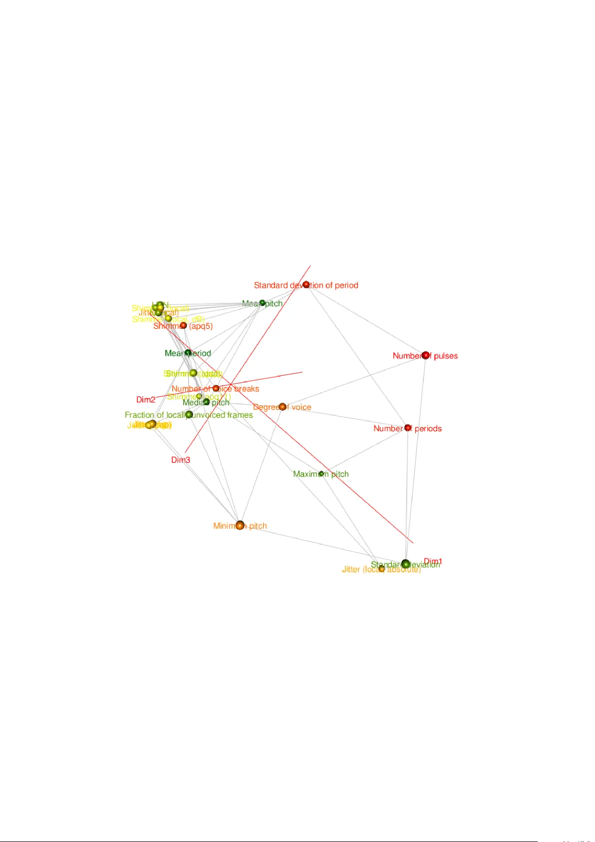
Original Paper
Loading high-quality paper...
Comments & Academic Discussion
Loading comments...
Leave a Comment