RIPML: A Restricted Isometry Property based Approach to Multilabel Learning

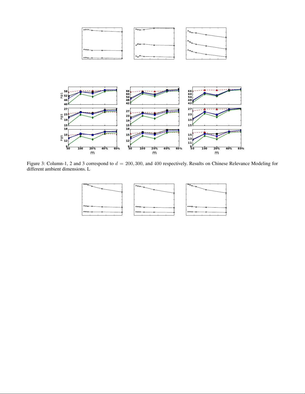
RIPML: A Restricted Isometry Pr operty based A ppr oach to Multilabel Lear ning Akshay Soni Y ahoo! Research, Sunnyv ale akshaysoni@yahoo-inc.com Y ashar Mehdad Airbnb, San Francisco yashar .mehdad@airbnb .com Abstract The multilabel learning problem with lar ge number of labels, features, and data-points has generated a tremendous interest recently . A recurring theme of these problems is that only a few labels are active in any giv en datapoint as compared to the total number of labels. Howe ver , only a small number of existing work take direct advantage of this inherent extreme sparsity in the label space. By the virtue of Restricted Isom- etry Pr operty (RIP), satisfied by many random ensembles, we propose a novel procedure for multilabel learning known as RIPML. During the training phase, in RIPML, labels are projected onto a random low-dimensional subspace follo wed by solving a least-square problem in this subspace. Inference is done by a k-nearest neighbor (kNN) based approach. W e demonstrate the effecti veness of RIPML by conducting ex- tensiv e simulations and comparing results with the state-of- the-art linear dimensionality reduction based approaches. 1 Introduction The task of multilabel learning is to predict a small set of labels associated with each datapoint out of all possible la- bels. Interest in these problems with large number of labels, features, and data-points has risen due to the applications in the area of image/video annotation [1], bioinformatics where a gene has to be associated with dif ferent functions [2], and entity recommendation for documents and images on a web- scale [3, 4]. Modern applications of multilabel learning are motiv ated by recommendation and ranking problems; for in- stance, in [5] each search engine query is treated as a label and the task is to get the most relev ant queries to a giv en webpage. Specific to Natural Language Processing (NLP), dev eloping highly scalable approaches for multilabel text categorization is an important task for variety of applica- tions such as relev ance modeling, entity recommendation, topic labeling and relation extraction. Recently , dimensionality reduction based approaches hav e gained popularity , for example, by using Compres- siv e Sensing (CS) [6, 7] and the state-of-the-art Low Rank Empirical Risk Minimization (LEML) algorithm [8]. There has also been advances made in non-linear dimensionality reduction based approaches such as the X1 algorithm [9]. These algorithms, ev en though being conceptually simple, Copyright c  2017, Association for the Advancement of Artificial Intelligence (www .aaai.org). All rights reserv ed. are still computationally heavy . F or instance, Compressiv e Sensing based approach has a very simple dimensionality re- duction procedure based on random projections, but require to solve a sparse reconstruction problem during prediction which is the bottleneck. T o address these issues, we propose a nov el approach that lev erages the advantages of both Compressiv e Sensing and the non-linear X1 algorithm. RIPML benefits from a sim- ple random projection based dimensionality reduction tech- nique during training as in Compressive Sensing and then use a kNN based approach during inference as recently pro- posed in the X1 algorithm [9]. The proposed approach is based on the fact that the number of activ e labels associ- ated with a datapoint is significantly smaller than the total number of labels, making the label vectors sparse. During training, we exploit this inherent sparsity in the label space by using random projections as a means to reduce the dimen- sionality of the label space. By the virtue of Restricted Isom- etry Property (RIP), satisfied by many random ensembles, the distances between the sparse label vectors are approx- imately preserved in the projected lo w-dimensional space as well. Giv en the training feature vectors, we then solve a least-squares problem to predict the low-dimensional label vectors. During inference, for a new datapoint, we use the output of the least-square problem to estimate the corresponding low-dimensional label vector and then use kNN in the low- dimensional label space to find the k -closest label vectors. In this way , the labels that occur man y times in these k - closest label vectors then become the estimated labels for this new datapoint. Howe ver , as noted by authors in [9], kNN is kno wn to be slow if the search for nearest neighbors in volve large number of data points which is generally the case. W e then lev erage the solution provided in [9] and clus- ter the training data into multiple clusters and apply RIPML to each cluster separately . 1.1 Related W ork The main advantages of embedding based methods is their simplicity , ease of implementation, strong theoretical foun- dations, the ability to handle label correlations, the ability to adapt to online and incremental scenarios, and the ability to work in a language/domain ignorant manner . The idea of Compressiv e Sensing based approaches [6, 7] is to project the high-dimensional label vector into a smaller random- subspace and then solve a sparse recov ery problem in this low-dimensional space. The state-of-the-art (LEML) algo- rithm [8] lev erages the lo w-rank of label matrix to learn the projection matrix and the back-projection matrix in order to estimate the label vectors by solving a single unified opti- mization problem. The X1 algorithm [9] builds on the assertion that the critical assumption made by most dimensionality reduction based methods that the training label matrix is low-rank is violated in almost all the real world applications. The au- thors propose a locally non-linear embedding technique to reduce the dimension of the label vectors while approxi- mately preserving the distances between them. Prediction is done by using kNN in this low-dimensional space over the training data. 2 RIPML 2.1 Background In order to formulate the problem and present our approach, we first note down the definition of RIP and few matrices which satisfy this property . Definition: A matrix Φ ∈ R m × n satisfy the ( k , δ ) -RIP for δ ∈ (0 , 1) , if (1 − δ ) k x k 2 2 ≤ k Φ x k 2 2 ≤ (1 + δ ) k x k 2 2 (1) for all k -sparse vector s x ∈ R n . While it is dif ficult to construct deterministic matrices which satisfy RIP , the best known guarantees arise from the random matrix theory . For example, follo wing random en- sembles satisfy RIP with high probability [10] • Gaussian matrix whose entries are i.i.d. N (0 , 1 /m ) i.e. distributed normally with variance 1 / √ m for m = O ( k log( n/k )) • Bernoulli matrix with i.i.d. entries over {± 1 / √ m } with m = O ( k log( n/k )) Note that if n is large and k is very small then we only need m  n to satisfy RIP , giving a very low-dimensional dis- tance preserving embedding. If a matrix Φ satisfy (2 k , δ ) - RIP , then for all k -sparse vectors x and y , we hav e (1 − δ ) k x − y k 2 2 ≤ k Φ ( x − y ) k 2 2 ≤ (1 + δ ) k x − y k 2 2 which essentially means that the distance between the pro- jected vectors Φ x and Φ y is close to the distance between the original vectors x and y . This distance preserving prop- erty of random projections is at the core of RIPML. It is to be noted that the classical Johnson and Linden- strauss Lemma [11] shows that any set of points can be embedded in a lower -dimensional space while preserving the distances between them. RIP specializes that result and prov es that some random ensembles indeed hav e this prop- erty , and can take advantage of the underlying sparsity to find a space of O ( k log( n/k )) dimension to embed n points that are k sparse. As noted above, there are many different random ensem- bles which satisfy RIP , but in this paper we report experi- mental results using Gaussian ensembles only . Algorithm 1 RIPML: Inference Inputs: T est point x new , no. of desired labels p , no. of nearest neighbors k , number of learners F , Z , b Ψ f for f ∈ [ F ] , Y Step 1: For each f ∈ [ F ] do: a) z f new = b Ψ f x new b) { i f 1 , i f 2 , . . . , i f k } ← kNN ( k ) in Z Step 3: D = 1 F k P F f =1 P i f k i = i f 1 y i Step 4: b y new ← T op p ( D ) Output: b y new 2.2 Algorithm T raining data is of the form { ( x i , y i ) , i = 1 , 2 , . . . , N } , where x i ∈ R d is the feature vector , y i ∈ { 0 , 1 } L is the binary label vector and L denotes the total number of labels. For  ∈ [ L ] 1 , y i [  ] = 1 denotes that the  th label is “present” and y i [  ] = 0 denotes otherwise. T raining Procedur e Step 1 – Label V ector Dimension- ality Reduction: First, we project the training label vectors into a lower -dimensional space while approximately pre- serving the distances between them. This by the virtue of sparsity of label vectors is achiev ed by using a RIP satisfy- ing matrix as a dimensionality reduction operator . That is, giv en a RIP satisfying matrix Φ ∈ R m × L , we get the low- dimensional label vectors as z i = Φ y i k y i k 2 = Φ e y i (2) where z i ∈ R m is the lo w-dimensional representation of y i . Note that the above matrix-vector product can be effi- ciently calculated by just adding entries of each row of Φ corresponding to the nonzero locations of y i and then nor- malizing the result by the square root of number of nonzero entries in y i . If there are s -nonzeros in y i , the abov e product can be computed in O ( sm ) operations rather then O ( mL ) operations, required if the label vectors were dense. Since we are operating under the assumption that s  L , the di- mensionality reduction procedure adopted by us is efficient and fast. W e normalize the label vectors in (2) in order to work with the cosine similarity as distance metric. Step 2 – Least-Squar es: Giv en ( x i , z i ) for i ∈ [ N ] , we want to learn a matrix Ψ ∈ R m × d such that z i ≈ Ψ x i for all i ∈ [ N ] . W e propose to solve following least- square problem to learn Ψ b Ψ = arg min Ψ 1 2 N X i =1 ( z i − Ψ x i ) 2 + λ k Ψ k 2 F (3) where λ ≥ 0 is the regularization parameter which controls the Frobenius norm 2 of the learned matrix. For reasonable feature dimension d , we can solve (3) in closed form, and if solving in closed form is not an option, we can use op- timization approaches like gradient descent to solve it it- erativ ely . The overall output of the training procedure is Z = [ z 1 , z 2 , . . . , z N ] ∈ R m × N and b Ψ . 1 Here and in rest of the paper, for a non-negati ve integer M , the notation [ M ] represents the set { 1 , 2 , . . . , M } . 2 For a matrix X ∈ R m × n , k X k 2 F = P i,j X 2 ij Since our approach is randomized by the choice of Φ , we can learn multiple models for different instances of Φ , and combine their predictions to produce a more accurate model. Let F be the number of learners, then our training procedure giv es us b Ψ f where f ∈ [ F ] . Unless stated otherwise F = 5 throughout the paper . Inference Procedure Giv en a ne w feature vector x new , we want to predict the labels associated with it. Gi ven b Ψ f for f ∈ [ F ] , the following tw o steps are ex ecuted: Step 1 – Get z f new ∈ R m : z f new = b Ψ f x new . Step 2 – Find kNN of z f new : Finds the indices of k vectors from Z which are closest to z f new in terms of squared dis- tance. Say those indices are i f 1 , i f 2 , . . . , i f k . Then we compute the empirical label distribution as 1 F k P F f =1 P i f k i = i f 1 y i out of which we can pick out the top- p locations corresponding to highest v alues and gi ve them as an estimate of the labels as- sociated with x new . W e use vanilla kNN for the e xperiments in this paper , but this step can be made scalable and fast by using techniques such as Locality Sensitive Hashing [12]. For certain random ensembles like Gaussian, the locality-sensiti ve functions are already well-known [13]. In order to keep the exposition simple, we make note of these approaches, b ut use simple kNN to do the experiments. 2.3 Scaling to Large Datasets Even though our training procedure is simple and scalable, kNN can be slow for datasets with large number of data points which increases the testing time. In order to tackle large datasets, we first cluster the feature vectors into C clusters using a simple procedure like KMeans. Then for each cluster c , we get the low-dimensional label vectors Z c (T raining – Step 1) and learn b Ψ c (T raining – Step 2). For a new test feature vector , we first find its cluster mem- bership by finding the cluster-center closest to it, and then apply our testing procedure by using Z c and b Ψ c for that cluster . 3 Experiments and Results 3.1 Experimental Settings Baselines: Since our approach is based on linear dimensionality-reduction, we compare it with other state-of- the-art linear dimensionality reduction based approaches: • LEML (Low rank Empirical risk minimization for Multi- Label Learning) with squared loss [8]. The implementa- tion of this algorithm was provided by the authors. • CPLST 3 (Conditional Principal Label Space T ransforma- tion) [14]. • CSSP (Column Subset Selection Problem) [15] 3 The implementation for CPLST and CSSP was taken from: https://github.com/hsuantien/mlc_lsdr Datasets: W e perform e xperiments on fiv e textual real world datasets. The first three are popular datasets that have been used in the previous works: Bibtex [3], EURLex [16], and Delicious [17] 4 . These datasets are already partitioned into train and test which we use directly for our experiments. W e call these group of datasets as MLL datasets. In order to further pro ve the generalizability and scalabil- ity of our approach, we conduct the same set of e xperiments on other datasets. These datasets were created and will be released as a by-product of our contribution to this w ork: -Relevance Modeling (Chinese Finance News) : a set of financial news documents in Chinese with their relev ant ticker symbols. In this dataset, each document is labeled with ticker symbols of the companies to which the docu- ment is rele vant. The annotation w as performed by an e xpert nativ e language editorial team. The e valuation results ov er these two datasets measure how well our approach deals with documents from other languages and emphasize the generalizability of our approach. -Entity Recommendation (English Wikipedia) : we randomly sampled one million documents from English W ikipedia and labeled the documents with entities. The con- cept of entity in this work is referred to any segment of text that is linked to another page in W ikipedia. W e then fil- tered out the entities which occurred less than 10 times in the entire dataset. Multilabel learning over such dataset is very challenging due to the number of labels (i.e., entities) in W ikipedia. This dataset measures how well our approach deals with very large number of labels and emphasize the scalability of our approach. For the document embeddings of the above mentioned two datasets, we use doc2vec [18] to learn dense lo w- dimensional vectors. W e train the embeddings of the words in documents using skip-bigram model [19] using hierarchi- cal softmax training. For the embedding of documents we exploit the distrib uted memory model since it usually per- forms well for most tasks [18]. The dimension, number of labels and other statistics for the datasets are shown in T able 1. Evaluation Criteria: Following the trail of the research in this field [8, 9, 14], we take precision at K (P@K) as our ev aluation criteria. Precision at K is the fraction of correct labels in the top- K label predictions. For the ease of com- parison with other research papers we use K = 1 , 3 and 5 in this paper . 3.2 Results on MLL datasets The P@1, P@3 and P@5 results are tab ulated in Figure 1. W e can observe that our results outperform the strong base- lines in Bibtex and EURLex datasets. Howe ver , for Deli- cious dataset, our approach performs worse than CPLST . W e suspect this might be due to the f act that the a verage number of nonzero labels per data-point is quite lar ge for this dataset and also the features are very sparse, see T able 1. 4 All of these standard datasets are av ailable online at: http: //mulan.sourceforge.net/datasets- mlc.html Dataset d avg. nnz( x ) L avg. nnz( y ) T otal Datapoints Train ( N ) T est Bibtex 1836 68 . 74 159 2 . 40 7395 4880 2515 EURLex 5000 236 . 69 3993 5 . 31 19314 17383 1931 Delicious 500 18 . 17 983 19 . 03 16091 12910 3181 Chinese Relev ance Modeling 100 − 400 dense 391 1 . 02 5011 4511 500 Entity Recommendation 400 dense 359524 32 . 55 510539 500539 10000 T able 1: Statistics of dif ferent datasets used in this paper . Here, avg. nnz( y ) denotes the average number of labels per data-point. Similarly , a vg. nnz( x ) denotes the average number of non-zero features per data-point. 4 5 5 0 5 5 6 0 6 5 P@1 2 1 2 5 2 9 3 3 3 7 P@3 5 0 1 0 0 2 0 % 4 0 % 6 0 % m 1 4 1 8 2 2 2 6 P@5 6 0 6 2 6 4 6 6 5 0 5 3 5 6 5 9 5 0 1 0 0 2 0 % 4 0 % 6 0 % m 4 6 4 9 5 2 5 5 5 8 3 4 4 2 5 0 5 8 6 6 2 5 3 3 4 1 4 9 5 7 6 5 5 0 1 0 0 2 0 % 4 0 % 6 0 % m 2 0 2 8 3 6 4 4 5 2 6 0 Figure 1: Column 1, 2 and 3 represent Bibtex, Delicious, and EURLex datasets. Results for standard datasets: Bibtex, Delicious and EURLex. Legend: RIPML (- - N - -) , LEML (–  –), CPLST (– • –) , CSSP (–  –) . Y -axis: m = [50, 100, 20% of L , 40% of L , 80% of L ]. Here k = 5 . An interesting point to note from these results is that RIPML remains stable with varying m while other ap- proaches start with a lower precision for small m and then gradually improve with increasing m . This stability of RIPML can be attributed to RIP which allows to obtain a sta- ble distance-preserving embedding with m = O ( s log ( s )) where s is the maximum number of nonzeros in the label vectors. Thus, increasing m abov e a certain threshold only results in a marginal improvement. This property also allows RIPML to perform better than other algorithms for small m – see results for Bibtex, and EURLes for m = 50 or 100 . Figure 2 shows the v ariation of precision with number of nearest neighbors used for kNN. Bibtex and Delicious are quite stable with the choice of number of nearest neighbors but EURLex performs better with smaller number of nearest neighbors. 3.3 Results on Relev ance Modelling Datasets In this work, we obtain the low-dimensional embedding of documents using the method described in Section 3 with window sizes of 10. In order to see the effect of dimensions, we also experiment with four low-dimensional models (200, 300 and 400 dims). During training the document embed- dings we limit the number of iterations to 10 to increase the efficienc y . Figure 3 shows the results for Chinese relev ance modeling datasets with different ambient dimensions. All these results are av eraged o ver 5 random train-test splits. It is interest- ing to note that RIPML performs better than CPLST and CSSP always, but performs worse than LEML in certain cases. Another interesting observation is that even though the P@1 is good for these datasets, P@5 drops significantly for all the approaches. This is due to the very low number of relev ant tickers for each document (average number of rele- vant tickers per document is about 1 ). In conclusion, RIPML performs well for detecting the relev ant tickers, considering that our approach doesn’t require any linguistic preprocess- ing which is one of the main challenges in multilingual NLP community . Figure 4 shows the variation of precision with respect to number of nearest neighbors used during prediction for these two datasets. For these datasets, small number of nearest neighbors results in a better precision, due to v ery less av er- age number of relev ant ticker symbols per document. 3.4 Results on Entity Recommendation Dataset W e created this dataset from W ikipedia to sho w how cluster- ing can be used to scale to big datasets with v ery lar ge num- ber of labels, and the effect of clustering on performance. In order to get a baseline to compare the effect of clustering, we first conduct experiments without using the clustering step. Giv en that our training and testing procedure is very effi- cient, we were able to train our model on this data in less than 3 minutes on a laptop 5 . W e used 10000 data points for testing and rest for training. Our results are av eraged ov er 5 random train-test split. It took approximately 72 millisec- 5 Apple MacBook Pro with 2.5GHz Intel Core i7 and 16 GB RAM. knn 0 20 40 60 80 100 precision 25 30 35 40 45 50 55 60 65 knn 0 20 40 60 80 100 precision 52 54 56 58 60 62 64 knn 0 20 40 60 80 100 precision 35 40 45 50 55 60 65 70 Figure 2: Column 1, 2 and 3 represent Bibte x, Delicious, and EURLe x datasets. Ro w-1: precision@ { 1,3,5 } vs. k for kNN. Here –  –, –  – and – ◦ – corresponds to precision@1, 3 and 5 respectiv ely . Here m = 100 . 4 0 4 6 5 2 5 8 P@1 1 5 1 9 2 3 2 7 P@3 5 0 1 0 0 2 0 % 4 0 % 6 0 % m 9 1 2 1 5 1 8 P@5 4 2 4 8 5 4 6 0 6 6 1 5 1 9 2 3 2 7 5 0 1 0 0 2 0 % 4 0 % 6 0 % m 9 1 2 1 5 1 8 4 2 4 8 5 4 6 0 6 6 1 5 1 9 2 3 2 7 5 0 1 0 0 2 0 % 4 0 % 6 0 % m 9 1 1 1 3 1 5 Figure 3: Column-1, 2 and 3 correspond to d = 200 , 300 , and 400 respectiv ely . Results on Chinese Relev ance Modeling for different ambient dimensions. Legend: RIPML (- - N - -) , LEML (–  –), CPLST (– • –) , CSSP (–  –) . X-axis: m = [50, 100, 20% of L , 40% of L , 80% of L ]. Here k = 5 . knn 0 20 40 60 80 100 precision 10 15 20 25 30 35 40 45 50 55 60 knn 0 20 40 60 80 100 precision 10 20 30 40 50 60 70 knn 0 20 40 60 80 100 precision 10 20 30 40 50 60 70 Figure 4: Column-1, 2 and 3 correspond to d = 200 , 300 , and 400 respectiv ely . Row-1: precision@ { 1,3,5 } vs. k for kNN for Chinese T icker dataset Here –  –, –  – and – ◦ – corresponds to precision@1, 3 and 5 respectiv ely . Here m = 100 . onds to predict labels for each test data point. W e are not pro- viding any comparison for this dataset with other approaches because we were not able to train a model within reasonable amount of time. In order to improve the performance for this challeng- ing dataset, we then applied kMeans clustering algorithm to cluster the training data (features) into different number of clusters and trained RIPML on each of the clusters sepa- rately by borrowing ideas from [9]. For ev ery test data-point, we first figure out which cluster it belongs to by finding the nearest cluster center and then apply the kNN based pre- diction procedure on that cluster . Clustering helps us in two ways – it makes prediction faster by allowing us to do kNN on a small amount of data and it also increases the prediction accuracy . This is evident from the results shown in T able 2 where we present precision for varying number of clusters. Going from no clustering to around 43 clusters increases the precision by about 10% . W ith 43 clusters it took ∼ 7 min- utes to train and approximately 6 . 5 milliseconds to predict labels for each test data point. 4 Conclusions In this paper , we presented a nov el, scalable, and general multilabel learning algorithm based on random-projections and kNN called RIPML. W e demonstrated its performance on six different real world datasets which includes three pop- ular and three ne w datasets. The new datasets would also be released for the use of research community as a part of this work. W e would like to extend our algorithm to e xplore the problem of missing label cases. W e also plan to study the im- pact of using different RIP , satisfying random/deterministic ensembles. Moreover we will in vestigate the performance of other loss functions for the regression phase. Entity Recommendation (d = 400) Clusters = 1 Clusters = 25 Clusters = 43 Clusters = 56 m P@1 P@3 P@5 P@1 P@3 P@5 P@1 P@3 P@5 P@1 P@3 P@5 50 31.02 23.60 20.20 39.42 31.72 27.61 41.72 33.67 29.32 41.23 33.69 29.54 100 33.55 25.58 21.70 42.10 34.24 29.89 44.11 36.08 31.39 43.91 36.16 31.65 250 35.76 27.20 23.46 44.44 35.81 31.38 46.28 37.95 33.15 46.30 37.92 33.45 T able 2: Results on Entity Recommendation dataset. Clusters = 1 means that clustering step was not done. References [1] G.-J. Qi, X.-S. Hua, Y . Rui, J. T ang, T . Mei, and H.- J. Zhang, “Correlativ e multi-label video annotation, ” in Pr oceedings of the 15th ACM International Confer- ence on Multimedia , MM ’07, (New Y ork, NY , USA), pp. 17–26, A CM, 2007. [2] Z. Barutcuoglu, R. E. Schapire, and O. G. T royan- skaya, “Hierarchical multi-label prediction of gene function, ” Bioinformatics , vol. 22, pp. 830–836, Apr . 2006. [3] I. Katakis, G. Tsoumakas, and I. Vlahav as, “Multil- abel text classification for automated tag suggestion, ” in In: Pr oceedings of the ECML/PKDD-08 W orkshop on Discovery Challenge , 2008. [4] M. R. Boutell, J. Luo, X. Shen, and C. M. Brown, “Learning multi-label scene classification, ” P attern Recognition , v ol. 37, no. 9, pp. 1757 – 1771, 2004. [5] R. Agrawal, A. Gupta, Y . Prabhu, and M. V arma, “Multi-label learning with millions of labels: Recom- mending adv ertiser bid phrases for web pages, ” in Pr oceedings of the 22Nd International Conference on W orld W ide W eb , WWW ’13, (New Y ork, NY , USA), pp. 13–24, A CM, 2013. [6] D. Hsu, S. M. Kakade, J. Langford, and T . Zhang, “Multi-label prediction via compressed sensing, ” CoRR , vol. abs/0902.1284, 2009. [7] A. Kapoor , R. V iswanathan, and P . Jain, “Multil- abel classification using bayesian compressed sens- ing, ” pp. 2645–2653, 2012. [8] H.-F . Y u, P . Jain, P . Kar , and I. S. Dhillon, “Large-scale Multi-label Learning with Missing Labels, ” in ICML , 2014. [9] K. Bhatia, H. Jain, P . Kar , P . Jain, and M. V arma, “Lo- cally non-linear embeddings for extreme multi-label learning, ” CoRR , v ol. abs/1507.02743, 2015. [10] M. Rudelson and R. V ershynin, “Sparse reconstruc- tion by con ve x relaxation: Fourier and gaussian mea- surements, ” in Information Sciences and Systems, 2006 40th Annual Conference on , pp. 207–212, IEEE, 2006. [11] S. Dasgupta and A. Gupta, “ An elementary proof of a theorem of johnson and lindenstrauss, ” Random Struc- tur es & Algorithms , vol. 22, no. 1, pp. 60–65, 2003. [12] P . Indyk and R. Motwani, “ Approximate nearest neigh- bors: towards removing the curse of dimensionality , ” in Pr oceedings of the thirtieth annual A CM symposium on Theory of computing , pp. 604–613, A CM, 1998. [13] M. Datar , N. Immorlica, P . Indyk, and V . Mirrokni, “Locality-sensitiv e hashing scheme based on p-stable distributions, ” in Pr oceedings of the twentieth annual symposium on Computational geometry , pp. 253–262, A CM, 2004. [14] Y .-n. Chen and H.-t. Lin, “Feature-aware label space dimension reduction for multi-label classification, ” in Advances in Neural Information Pr ocessing Systems 25 (F . Pereira, C. J. C. Burges, L. Bottou, and K. Q. W einberger , eds.), pp. 1529–1537, Curran Associates, Inc., 2012. [15] W . Bi and J. Kw ok, “Efficient multi-label classification with many labels, ” in Pr oceedings of the 30th Inter- national Conference on Machine Learning (ICML-13) (S. Dasgupta and D. Mcallester, eds.), vol. 28, pp. 405– 413, JMLR W orkshop and Conference Proceedings, May 2013. [16] E. Loza Menc ´ ıa and J. F ¨ urnkranz, “Efficient mul- tilabel classification algorithms for large-scale prob- lems in the legal domain, ” in Semantic Pr ocessing of Le gal T exts – Wher e the Language of Law Meets the Law of Language (E. Francesconi, S. Monte- magni, W . Peters, and D. T iscornia, eds.), vol. 6036 of Lectur e Notes in Artificial Intelligence , pp. 192– 215, Springer-V erlag, 1 ed., May 2010. accompany- ing EUR-Le x dataset a vailable at http://www.ke. tu- darmstadt.de/resources/eurlex . [17] G. Tsoumakas, I. Katakis, and I. Vlaha vas, “Effec- tiv e and Ef ficient Multilabel Classification in Domains with Lar ge Number of Labels, ” in Pr oc. ECML/PKDD 2008 W orkshop on Mining Multidimensional Data (MMD’08) , p. XX, 2008. [18] Q. Le and T . Mik olov , “Distributed representations of sentences and documents, ” in Pr oceedings of the 31st International Conference on Machine Learning (ICML-14) (T . Jebara and E. P . Xing, eds.), pp. 1188– 1196, JMLR W orkshop and Conference Proceedings, 2014. [19] T . Mikolov , K. Chen, G. Corrado, and J. Dean, “Ef- ficient estimation of word representations in vector space, ” CoRR , v ol. abs/1301.3781, 2013.