Multigrid with rough coefficients and Multiresolution operator decomposition from Hierarchical Information Games

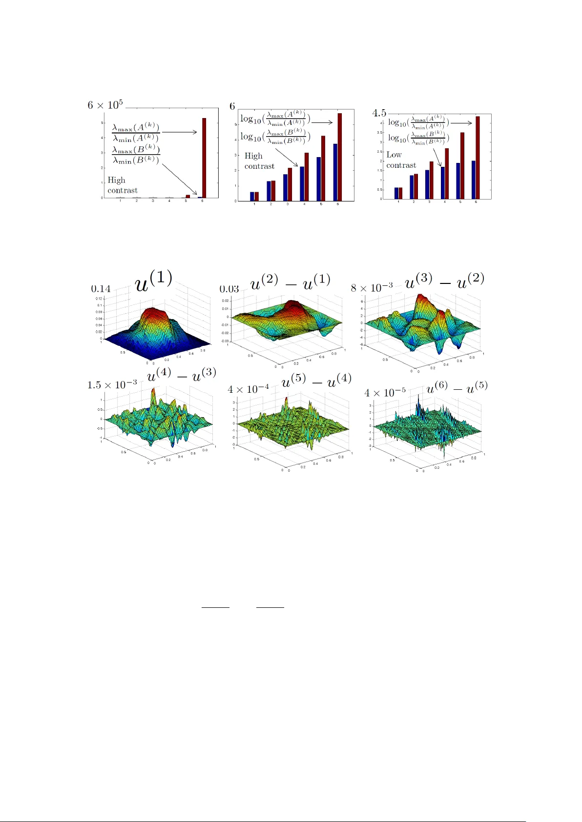
Multigrid with rough co eﬃcien ts and Multiresolution op erator decomp osition from Hierarc hical Information Games Houman Owhadi ∗ F ebruary 13, 2017 Abstract W e in tro duce a near-linear complexit y (geometric and meshless/algebraic) multi- grid/m ultiresolution metho d for PDEs with rough ( L ∞ ) co eﬃcien ts with rigorous a-priori accuracy and p erformance estimates. The metho d is discov ered through a decision/game theory formulation of the problems of (1) iden tifying restriction and in terp olation operators (2) reco v ering a signal from incomplete measurements based on norm constrain ts on its image under a linear operator (3) gambling on the v alue of the solution of the PDE based on a hierarch y of nested m easuremen ts of its solution or source term. The resulting elemen tary gam bles form a hierar- c hy of (deterministic) basis functions of H 1 0 (Ω) (gamblets) that (1) are orthogonal across subscales/subbands with resp ect to the scalar product induced by the energy norm of the PDE (2) enable sparse compression of the solution space in H 1 0 (Ω) (3) induce an orthogonal multiresolution op erator decomp osition. The op erating dia- gram of the multigrid method is that of an inv erted pyramid in which gamblets are computed lo cally (by virtue of their exp onen tial decay), hierarc hically (from ﬁne to coarse scales) and the PDE is decomp osed into a hierarch y of indep endent lin- ear systems with uniformly b ounded condition num b ers. The resulting algorithm is parallelizable b oth in space (via lo calization) and in bandwith/subscale (subscales can b e computed indep enden tly from eac h other). Although the metho d is deter- ministic it has a natural Ba yesian interpretation under the measure of probability emerging (as a mixed strategy) from the information game form ulation and mul- tiresolution approximations form a martingale with resp ect to the ﬁltration induced b y the hierarch y of nested measuremen ts. 1 In tro duction 1.1 Scien tiﬁc disco v ery as a decision theory problem The pro cess of scientiﬁc discov ery is oftentimes based on in tuition, trial and error and plain guesswork. This pap er is motiv ated b y the question of the existence of a rational ∗ California Institute of T ec hnology , Computing & Mathematical Sciences , MC 9-94 Pasadena, CA 91125, owhadi@caltec h.edu 1 decision framew ork that could b e used to facilitate/guide this process, or turn it, to some degree, in to an algorithm. In exploring this question, we will consider the problem of ﬁnding a metho d for solving (up to a pre-sp eciﬁed lev el of accuracy) PDEs with rough ( L ∞ ) co eﬃcien ts as fast as p ossible with the following protot ypical PDE (and its p ossible discretization o ver a ﬁne mesh) as an example ( − div  a ( x ) ∇ u ( x )  = g ( x ) x ∈ Ω; g ∈ L 2 (Ω) , or g ∈ H − 1 (Ω) u = 0 on ∂ Ω , (1.1) where Ω is a b ounded subset of R d (of arbitrary dimension d ∈ N ∗ ) with piecewise Lipsc hitz b oundary , a is a symmetric, uniformly elliptic d × d matrix with entries in L ∞ (Ω) and suc h that for all x ∈ Ω and l ∈ R d , λ min ( a ) | l | 2 ≤ l T a ( x ) l ≤ λ max ( a ) | l | 2 . (1.2) Although multigrid metho ds [ 41 , 16 , 50 , 51 , 101 ] are now well known as the fastest for solving elliptic boundary-problems and ha v e successfully been generalized to other t yp es of PDEs and computational problems [ 123 ], their con vergence rate can b e sev erely aﬀected by the lac k of regularit y of the co eﬃcients [ 37 , 114 ]. F urthermore, although sig- niﬁcan t progress has b een ac hieved in the dev elopment of m ultigrid methods that are, to some degree, robust with resp ect to meshsize and lac k of smo othness (we refer in partic- ular to algebraic m ultigrid [ 94 ], m ultilev el ﬁnite elemen t splitting [ 124 ], hierarc hical basis m ultigrid [ 9 , 24 ], multilev el preconditioning [ 106 ], stabilized hierarc hical basis metho ds [ 107 , 109 , 110 ], energy minimization [ 65 , 114 , 122 , 121 , 108 ] and homogenization based metho ds [ 37 , 34 ]), the design of m ultigrid metho ds that are pro v ably robust with resp ect to rough ( L ∞ ) co eﬃcien ts has remained an op en problem of practical imp ortance [ 17 ]. Alternativ e hierarc hical strategies for the resolution of ( 1.1 ) are (1) w av elet based metho ds [ 18 , 15 , 3 , 29 , 38 ] (2) the F ast Multip ole Metho d [ 49 ] and (3) Hierarchical ma- trices [ 52 , 11 ]. Although metho ds based on (classical) wa v elets achiev e a m ultiresolution compression of the solution space of ( 1.1 ) in L 2 and although approximate w av elets and approximate L 2 pro jections can stabilize hierarc hical basis metho ds [ 109 , 110 ], their applications to ( 1.1 ) are limited b y the facts that (a) the underlying w av elets can p er- form arbitrarily badly [ 7 ] in their H 1 0 (Ω) approximation of the solution space and (b) the op erator ( 1.1 ) do es not preserv e the orthogonality betw een subscales/subbands with classical wa v elets. The F ast Multip ole Metho d and hierarc hical matrices exploit the prop ert y that sub-matrices of the in verse discrete op erator are lo w rank aw ay from the diagonal. This low rank prop ert y can b e rigorously prov en for ( 1.1 ) (based on the ap- pro ximation of its Green’s function by sums of pro ducts of harmonic functions [ 10 ]) and leads to pro v able conv ergence (with rough co eﬃcien ts), up to the pre-sp eciﬁed level of accuracy  in L 2 -norm, in O ( N ln 6 N ln 2 d +2 1  ) op erations ([ 10 ] and [ 11 , Thm. 2.33 and Thm. 4.28]). Can the problem of ﬁnding a fast solver for ( 1.1 ) b e, to some degree, reform ulated as an Uncertaint y Quantiﬁcation/Decision Theory problem that could, to some degree, b e solved as suc h in an automated fashion? Can discov ery b e computed? Although these questions ma y seem unorthodox their answ er app ears to b e p ositive: this 2 pap er shows that this reformulation is p ossible and leads to a m ultigrid/multiresolution metho d/algorithm solving ( 1.1 ), up to the pre-sp eciﬁed level of accuracy  in H 1 -norm (i.e. ﬁnding u app suc h that k u − u app k H 1 0 (Ω) ≤  k g k H − 1 (Ω) for an arbitrary g decomp osed o ver N degrees of freedom), in O  N ln 3 d  max( 1  , N 1 /d )  op erations (for  ∼ N − 1 /d , the hierarc hical matrix method achiev es  -accuracy in L 2 norm in O ( N ln 2 d +8 N ) op- erations and the prop osed multiresolution metho d ac hiev es  -accuracy in H 1 norm in O ( N ln 3 d N ) op erations). F or subsequent solves (i.e. if ( 1.1 ) needs to b e solved for more than one g ) then the prop osed multiresolution metho d achiev es accuracy  ≈ N − 1 d in H 1 -norm in O ( N ln d +1 N ) operations (w e refer to Subsection 5.4 and in particular to T able 1 for a detailed complexity analysis of the prop osed metho d, whic h can also ac hieve sublinear complexity if one only requires L 2 -appro ximations). The core mechanism supp orting the complexity of the metho d presented here is the fast decomp osition of H 1 0 (Ω) into a direct sum of linear subspaces that are orthogonal (or near-orthogonal) with resp ect to the energy scalar pro duct and ov er whic h ( 1.1 ) has uniformly b ounded condition n um b ers. It is, to some degree, surprising that this decomp osition can b e achiev ed in near linear complexity and not in the complexity of an eigenspace decomp osition. Naturally [ 86 ], this decomp osition can b e applied to the fast simulation of the w av e and parab olic equations asso ciated to ( 1.1 ) or to its fast diagonalization. The essen tial step b ehind the automation of the discov ery/design of scalable n umer- ical solvers is the observ ation that fast computation requires rep eated computation with partial information (and limited resources) o ver hierarchies of levels of complexit y and the reformulation of this pro cess as that of pla ying underlying hierarchies of adv ersarial information games [ 111 , 112 ]. Although the problem of ﬁnding a fast solver for ( 1.1 ) may app ear disconnected from that of ﬁnding statistical estimators or making decisions from data sampled from an underlying unkno wn probabilit y distribution, the proposed game theoretic reformulation is, to some degree, analogous to the one dev elop ed in W ald’s Decision Theory [ 113 ], eviden tly inﬂuenced b y V on Neumann’s Game Theory [ 111 , 112 ] (the generalization of w orst case Uncertaint y Quan tiﬁcation analysis [ 83 ] to sample data/mo del uncertaint y requires an analogous game theoretic form ulation [ 80 ], see also [ 79 ] for how the underlying calculus could b e used to guide the discov ery of new Selb erg identities). W e also refer to subsection 1.3 for a review of the corresp ondence b et ween statistical inference and n umerical approximation. 1.2 Outline of the pap er The essential diﬃculty in generalizing the multigrid concept to PDEs with rough co eﬃ- cien ts lies in the fact that the in terp olation (do wnscaling) and restriction (upscaling) op- erators are, a priori, unknown. Indeed, in this situation, piecewise linear ﬁnite-elements can p erform arbitrarily badly [ 7 ] and the design of the interpolation op erator requires the iden tiﬁcation of accurate basis elements adapted to the microstructure a ( x ). This identiﬁcation problem has also b een the essential diﬃculty in numerical homoge- 3 nization [ 117 , 6 , 4 , 18 , 59 , 33 , 84 , 17 ]. Although inspired by classical homogenization ideas and concepts (such as oscillating test functions [ 68 , 36 , 35 ], cell problems/correctors and eﬀectiv e co eﬃcien ts [ 13 , 90 , 1 , 72 , 39 , 46 ], harmonic co ordinates [ 61 , 6 , 4 , 76 , 12 , 2 , 84 ], compactness by comp ensation [ 100 , 45 , 67 , 14 ]) an essential goal of n umerical homoge- nization has b een the numerical approximation of the solution space of ( 1.1 ) with arbi- trary rough coeﬃcients [ 84 ], i.e., in particular, without the assumptions found in classical homogenization, such as scale separation, ergo dicit y at ﬁne scales and  -sequences of op- erators (otherwise the resulting metho d could lack robustness to rough co eﬃcients, ev en under the assumption that co eﬃcien ts are stationary [ 8 ]). F urthermore, to envisage ap- plications to multigrid metho ds, the computation of these basis functions must also b e pro v ably lo calized [ 5 , 85 , 64 , 48 , 87 , 58 ] and compatible with nesting strategies [ 87 ]. In [ 77 ], it has b een shown that this pro cess of identiﬁcation (of accurate basis elements for n umerical homogenization), could, in principle, b e guided through its reform ulation as a Ba yesian Inference problem in whic h the source term g in ( 1.1 ) is replaced b y noise ξ and one tries to estimate the v alue of the solution at a giv en p oin t based on a ﬁnite num b er of observ ations. In particular it was found that Rough Polyharmonic Splines [ 87 ] and P olyharmonic Splines [ 54 , 30 , 31 , 32 ] can b e re-disco vered as solutions of Gaussian ﬁlter- ing problems. This pap er is inspired by the suggestion that this link b et w een n umerical homogenization and Ba yesian Inference (and the link b et ween Numerical Quadrature and Bay esian Inference [ 92 , 27 , 97 , 74 , 75 ]) are not coincidences but particular instances of mixed strategies for underlying information games and that optimal or near optimal metho ds could b e obtained b y identifying such games and their optimal strategies. The process of iden tiﬁcation of these games starts with the (Information Based Com- plexit y [ 119 ]) notion that computation can only b e done with partial information. F or instance, since the operator ( 1.1 ) is inﬁnite dimensional, one cannot directly compute with u ∈ H 1 0 (Ω) but only with ﬁnite-dimensional fe atur es of u . An example of suc h ﬁnite- dimensional features is the m -dimensional v ector u m := ( R Ω uφ 1 , . . . , R Ω uφ m ) obtained b y integrating the solution u of ( 1.1 ) against m test/measurement functions φ i ∈ L 2 (Ω). Ho wev er to ac hieve an accurate appro ximation of u through computation with u m one m ust ﬁll the information gap b et ween u m and u (i.e. construct an interpolation op erator giving u as a function of u m ). W e will, therefore, reformulate the identiﬁcation of this in terp olation op erator as a non-co operative (min max) game where Play er I chooses the source term g ( 1.1 ) in an admissible set/class (e.g. the unit ball of L 2 (Ω)) and Play er I I is sho wn u m and m ust approximate u from these incomplete measurements. Using the energy norm k u k 2 a := Z Ω ∇ u T ( x ) a ( x ) ∇ u ( x ) dx, (1.3) to quan tify the accuracy of the recov ery and calling u ∗ Pla yer I’s b et (on the v alue of u ), the ob jectiv e of Play er I is to maximize the appro ximation error k u − u ∗ k a , while the ob jective of Pla yer II is to minimize it. A remark able result from Game Theory (as developed by V on Neumann [ 111 ], V on Neumann and Morgenstern [ 112 ] and Nash [ 70 ]) is that optimal strategies for deterministic zero sum ﬁnite games are mixed (i.e. randomized) strategies. Although the information game described ab o ve is zero sum, 4 it is not ﬁnite. Nev ertheless, as in W ald’s Decision Theory [ 113 ], under suﬃcien t regu- larit y conditions it can b e made compact and therefore approximable b y a ﬁnite game. Therefore although the information game describ ed ab ov e is purely deterministic (and has no a priori connection to statistical estimation), under compactness (and contin uity of the loss function), the b est strategy for Play er I is to pla y at random by placing a probabilit y distribution π I on the set of candidates for g (and select g as a sample from π I ) and the optimal strategy for Pla yer I I is to place a probability distribution π I I on the set of candidates for g and approximate the solution of ( 1.1 ) by the exp ectation of u (under π I I used as a prior distribution) conditioned on the measurements R Ω uφ i . Although the estimator employ ed by Pla yer II may b e called Ba yesian, the game describ ed here is not (i.e. the choice of Play er I might b e distinct from that of Play er I I) and Play er I I m ust solv e a min max optimization problem o ver π I and π I I to identify an optimal prior distribution for the B a yesian estimator (a careful choice of the prior also app ears to b e imp ortan t due to the p ossible high sensitivity of p osterior distributions [ 81 , 79 , 82 ]). Although solving the min max problem ov er π I and π I I ma y b e one wa y of determining the strategy of Pla yer I I, it will not b e the metho d emplo yed here. W e will instead analyze the error of Play er I I’s appro ximation as a function of Pla yer I I’s prior and the source term g pick ed by Pla yer I. F urthermore, to preserve the linearity of the calculations we will restrict Play er I I’s decision space (the set of p ossible priors π I I ) to Gaussian priors on the source term g . Since the resulting analysis is indep endent of the structure of ( 1.1 ) and solely dep ends on its linearity we will ﬁrst p erform this inv esti- gation, in Section 2 , in the algebraic framew ork of linear systems of equations, identify Pla yer II’s optimal mixed strategy and sho w that it is c haracterized b y deterministic optimal reco very and accuracy prop erties. The mixed strategy iden tiﬁed in Section 2 will then b e applied in 3 to the n umerical homogenization of ( 1.1 ) and the disco very of in terp olation in terp olators. In particular, it will b e shown that the resulting elementary gam bles form a set of deterministic basis functions (gamblets) characterized by (1) op- timal recov ery and accuracy prop erties (2) exp onen tial decay (enabling their lo calized computation) (3) robustness to high contrast. T o compute fast, the game presen ted ab o v e must not b e limited to ﬁlling the infor- mation gap b et w een u m ∈ R m and u ∈ H 1 0 (Ω). This game m ust be pla yed (and repeated) o ver hierarc hies of lev els of complexity (e.g. one must ﬁll information gaps b et w een R 4 and R 16 , then R 16 and R 64 , etc...). W e will therefore, in Section 4 , consider the (hier- arc hical) game where Play er I chooses the r.h.s of ( 1.1 ) and Play er I I must (iteratively) gam ble on the v alue of its solution based on a hierarch y of nested measuremen ts of u (from coarse to ﬁne measurements). Under Play er I I’s mixed strategy (identiﬁed in Sec- tion 2 and used in Section 3 ), the resulting sequence of multi-resolution approximations forms a martingale. Conditioning and the indep endence of martingale increments lead to the hierarch y of nested interpolation op erators and to the multiresolution orthogonal decomp osition of ( 1.1 ) into indep enden t linear systems of uniformly b ounded condition n umbers. The resulting elementary gambles (gamblets) (1) form a hierarch y of nested basis functions leading to the orthogonal decomp osition (in the scalar pro duct of the energy norm) of H 1 0 (Ω) (2) enable the sparse compression of the solution space of ( 1.1 ) 5 (3) can b e computed and stored in near-linear complexity by solving a nesting of linear systems with uniformly b ounded condition num b ers (4) enable the computation of the solution of ( 1.1 ) (or its hyperb olic or parab olic analogues) in near-linear complexity . The implemen tation and complexit y of the algorithm are discussed in Section 5 with n umerical illustrations. 1.3 On the corresp ondence b et ween statistical inference and n umerical appro ximation As exp osed by Diaconis [ 27 ], the inv estigation of the corresp ondence b etw een statisti- cal inference and numerical approximation can be traced bac k to Poincar ´ e’s course in Probabilit y Theory [ 92 ]. It is useful to recall Diaconis’ comp elling example [ 27 ] as an illustration of this conection. Let f : [0 , 1] → R b e a giv en function and assume that w e are interested in the numerical approximation of R 1 0 f ( t ) dt . The Bay esian approach to this quadrature problem is to (1) Put a prior (probabilit y distribution) on con tin uous functions C [0 , 1] (2) Calculate f at x 1 , x 2 , . . . , x n (to obtain the data ( f ( x 1 ) , . . . , f ( x n ))) (3) Compute a p osterior (4) Estimate R 1 0 f ( t ) dt by the Ba yes rule. If the prior on C [0 , 1] is that of a Brownian Motion (i.e. f ( t ) = B t where B t is a Bro wnian motion and B 0 is normal), then E  f ( x )   f ( x 1 ) , . . . , f ( x n )  is the piecewise linear in terp olation of f b et ween the p oin ts x 1 , . . . , x n and one re-discov ers the trap ezoidal quadrature rule. If the prior on C [0 , 1] is that of the ﬁrst in tegral of a Brownian Motion (i.e. f ( t ) ∼ R t 0 B s ds ) then the p osterior E  f ( x )   f ( x 1 ) , . . . , f ( x n )  is the cubic spline interpolan t and integrating k times yields splines of order 2 k + 1. Subsequen t to P oincar´ e’s early disco very [ 92 ], Sul’din [ 102 ] and (in particular) Larkin [ 62 ] initiated the systematic inv estigation of the corresp ondence b et ween conditioning Gaussian measures/pro cesses and n umerical appro ximation. As noted by Larkin [ 62 ], de- spite Sard’s in tro duction of probabilistic concepts in the theory of linear approximation [ 95 ], and Kimeldorf and W ahba’s exp osition [ 60 ] of the correspondence betw een Ba yesian estimation and spline smo othing/interpolation, the application of probabilistic concepts and techniques to numerical in tegration/approximation “attracted little attention among n umerical analysts” (p erhaps due to the counterin tuitive nature of the pro cess of random- izing a known function). Ho wev er, a natural framew ork for understanding this pro cess of randomization can b e found in the pioneering w orks of W o ´ zniako wski [ 118 ], Pac kel [ 88 ], and T raub, W asilko wski, and W o ´ zniako wski [ 104 ] on Information Based Complex- it y [ 71 , 119 ], the branch of computational complexit y that studies the complexity of appro ximating con tinuous mathematical op erations with discrete and ﬁnite ones up a to sp eciﬁed level of accuracy . Indeed the concept that numerical implementation requires computation with partial information and limited resources emerges naturally from In- formation Based Complexity , where it is also augmen ted by concepts of contaminated and priced information asso ciated with, for example, truncation errors and the cost of n umerical op erations. In this framework, the p erformance of an algorithm op erating on incomplete information can b e analysed in the usual worst case setting or the a verage case (randomized) setting [ 93 , 73 ] with respect to the missing information. Although the measure of probability (on the solution space) employ ed in the av erage case setting 6 ma y b e arbitrary , as observed by Pac kel [ 88 ], if that measure is c hosen carefully (as the solution of a game theoretic problem) then the av erage case setting can b e interpreted as lifting a (w orst case) min max problem (where saddle p oin ts of pure strategies do not, in general, exist) to a min max problem ov er mixed (randomized) strategies (where saddle p oin ts do exist [ 111 , 112 ]). As exp osed b y Diaconis [ 27 ] (see also Sha w [ 97 ]) the randomized setting also establishes a corresp ondence b et w een Numerical Analysis and Ba yesian Inference providing a natural framew ork for the statistical description of nu- merical errors (in whic h conﬁdence in terv als can b e derived from p osterior distributions). F urthermore [ 89 , 27 ], classical min max numerical quadrature rules can b e formulated as solutions of Bay esian inference problems with carefully c hosen priors [ 27 ] and, as sho wn by O’Hagan [ 74 , 75 ], this corresp ondence can b e exploited to discov er new and useful n umerical quadratures rules. As envisioned by Skilling [ 99 ], b y placing a (care- fully chosen) probability distribution on the solution space of an ODE and conditioning on quadrature p oin ts, one obtains a p osterior distribution on the solution whose mean ma y coincide with classical numerical in tegrators such as Runge-Kutta methods [ 96 ]. As sho wn in [ 23 ] the statistical approac h is particularly w ell suited for chaotic dynamical systems for whic h deterministic worst case error b ounds may provide little information. While in [ 99 , 96 , 23 ] the probabilit y distribution is directly placed on the solutions space, for PDEs [ 77 ] argues that the prior distribution must b e placed on source terms (or on the image space of an integro-diﬀeren tial op erator) and propagated/ﬁltered through the in verse op erator to reﬂect the structure of the solution space. In particular [ 77 ] shows that this pro cess of ﬁltering noise with the inv erse op erator, when combined with con- ditioning, pro duces accurate ﬁnite-element basis functions for the solution space whose deterministic worst case errors can b e b ounded by standard deviation errors using the repro ducing k ernel structure of the co v ariance function of the ﬁltered Gaussian ﬁeld. As already witnessed in [ 23 , 96 , 77 , 56 , 55 , 19 , 25 ], it is natural to exp ect that the p ossibili- ties oﬀered b y com bining numerical uncertain ties/errors with mo del uncertain ties/errors in a uniﬁed framew ork will stimulate a resurgence of the statistical inference approach to n umerical analysis. 2 Linear Algebra with incomplete information 2.1 The reco very problem The problem of identifying interpolation op erators for ( 1.1 ) is equiv alent (after discretiza- tion or in the algebraic setting) to that of reco vering or approximating the solution of a linear system of equations from an incomplete set of measurements (coarse v ariables) giv en known norm constraints on the image of the solution. Let n ≥ 2 and A be a known real in vertible n × n matrix. Let b b e an unknown elemen t of R n . Our purp ose is to approximate the solution x of Ax = b (2.1) 7 based on the information that (1) x solves Φ x = y , (2.2) where Φ (the measurement matrix) is a kno wn, rank m , m × n real matrix such that m < n and y (the measurement v ector) is a known v ector of R m , and (2) the norm b T T − 1 b of b is known or b ounded by a kno wn constan t (e.g., b T T − 1 b ≤ 1), where T − 1 is a known p ositive deﬁnite n × n matrix (with T − 1 b eing the identit y matrix as a protot ypical example). Observ e that since m < n , the measuremen ts ( 2.2 ) are, a priori, not suﬃcien t to recov er the exact v alue x . As describ ed in Section 1 , b y formulating this reco very problem as a (non-co op erativ e) information game (where Play er I chooses b and Pla yer I I c ho oses an appro ximation x ∗ of x based on the observ ation Φ x ), one (Play er I I) is naturally lead to searc h for mixed strategy in the Bay esian class by placing a prior distribution on b . The purp ose of this section is to analyze the resulting approximation error and select the prior distribution accordingly . T o preserve the linearity (i.e. simplicity and computational eﬃciency) of calculations w e will restrict Play er I I’s decision space to Gaussian priors. 2.2 Pla y er I’s mixed strategy W e will therefore, in the ﬁrst step of the analysis, replace b in ( 2.1 ) by ξ , a cen tered Gaussian vector of R n with cov ariance matrix Q (which may b e distinct from T ) and consider the follo wing sto c hastic linear system AX = ξ . (2.3) The Bay esian answ er (a mixed strategy for Play er I I) to the recov ery problem of Section 2 is to appro ximate x by the conditional exp ectation E [ X | Φ X = y ]. Theorem 2.1. The solution X of ( 2.3 ) is a c enter e d Gaussian ve ctor of R n with c o- varianc e matrix K = A − 1 Q ( A − 1 ) T . (2.4) F urthermor e, X c onditione d on the value Φ X = y is a Gaussian ve ctor of R n with me an E [ X | Φ X = y ] = Ψ y , and of c ovarianc e matrix K Φ , wher e Ψ is the n × m matrix Ψ := K Φ T (Φ K Φ T ) − 1 , (2.5) and K Φ is the r ank n − m p ositive n × n symmetric matrix deﬁne d by K Φ := K − ΨΦ K . Pr o of. ( 2.4 ) simply follows from X = A − 1 ξ . Since X is a Gaussian v ector, E [ X | Φ X = y ] = Ψ y where Ψ is a n × m matrix minimizing the mean squared error E  | X − M Φ X | 2  o ver all n × m matrices M . W e ha ve E  | X − M Φ X | 2  = T race[ K ] + T race[ M Φ K Φ T M T ] − 2 T race[Φ K M ] whose minimum is ac hieved for M = Ψ as deﬁned by ( 2.5 ). The co- v ariance matrix of X given Φ X = y is then obtained b y observing that for v ∈ R n , v T K Φ v = E  | v T X − v T ΨΦ X | 2  = v T K v − v T ΨΦ K v . 8 2.3 V ariational/optimal recov ery prop erties and appro ximation error F or a n × n symmetric p ositiv e deﬁnite matrix M let  · , ·  M b e the (scalar) pro duct on R n deﬁned by: for u, v ∈ R n ,  u, v  M := u T M v and write k v k M :=  v , v  1 2 M the corresp onding norm. When M is the identit y matrix then we write  u, v  and k v k the corresp onding scalar pro duct and norm. F or a linear subspace V of R n w e write P V ,M for the orthogonal pro jections on to V with resp ect to the scalar pro duct  · , ·  M . F or a (p ossibly rectangular) matrix B w e write Im( B ) the image (range) of B and Ker( B ) the n ull space of B . F or an in teger n , let I n b e the n × n identit y matrix. Theorem 2.2. F or w ∈ R m , Ψ w is the unique minimizer of the fol lowing quadr atic pr oblem ( Minimize  v , v  K − 1 Subje ct to Φ v = w and v ∈ R n . (2.6) In p articular, v = Ψ y , the Bayesian appr oximation of the solution of ( 2.1 ) , is the unique minimizer of k Av k Q − 1 under the me asur ement c onstr aints Φ v = y . F urthermor e, it also holds true that (1) ΦΨ = I m (2) Im(Ψ) is the ortho gonal c omplement of Ker(Φ) with r esp e ct to the pr o duct  · , ·  K − 1 and (3) ΨΦ = P Im( K Φ T ) ,K − 1 and I n − ΨΦ = P Ker(Φ) ,K − 1 . Pr o of. First observ e that ( 2.5 ) implies that ΦΨ = I m where I m is the identit y m × m ma- trix. Therefore Φ(Ψ w ) = w . Note that ( 2.5 ) implies that for all z ∈ R m ,  Ψ z , v  K − 1 = z T  Φ K Φ T  − 1 Φ v . Therefore if v ∈ Ker(Φ) then  Ψ z , v  K − 1 = 0 for all z ∈ R m . Con- v ersely if  Ψ z , v  K − 1 = 0 for all z ∈ R m then v must b elong to Ker(Φ). Since the dimension of Im(Ψ) is m and that of Ker(Φ) is n − m we conclude that Im(Ψ) is the orthogonal complemen t Ker(Φ) with resp ect to the pro duct  · , ·  K − 1 and in particular,  Ψ w , v  K − 1 = 0 , ∀ w ∈ R m and ∀ v ∈ R n suc h that Φ v = 0 . (2.7) Let w ∈ R m and v ∈ R n suc h that Φ v = w . Since Ψ w − v ∈ Ker(Φ), it follo ws from ( 2.7 ) that  v , v  K − 1 =  Ψ w , Ψ w  K − 1 +  v − Ψ w , v − Ψ w  K − 1 . Therefore Ψ w is the unique minimizer of  v , v  K − 1 o ver all v ∈ R n suc h that Φ v = w . No w consider f ∈ R n , since Im(Ψ) = Im( K Φ T ) and Im(Ψ) is the orthogonal complemen t of Ker(Φ) with resp ect to the pro duct  · , ·  K − 1 , there exists a unique z ∈ R m and a unique g ∈ Ker(Φ) such that f = K Φ T z + g . Since ΨΦ = K Φ T (Φ K Φ T ) − 1 Φ, it follo ws that ΨΦ f = K Φ T z and ( I n − ΨΦ) f = g . W e conclude by observing that g = P Ker(Φ) ,K − 1 f . Theorem 2.3. F or v ∈ R n , w ∗ = Φ v is the unique minimizer of k v − Ψ w k K − 1 over al l w ∈ R m . In p articular, k v − ΨΦ v k K − 1 = min z ∈ R m k v − K Φ T z k K − 1 and if x is the solution of the original e quation ( 2.1 ) , then k x − Ψ y k K − 1 = min w ∈ R m k x − Ψ w k K − 1 = min z ∈ R m k x − K Φ T z k K − 1 . Pr o of. The proof follows by observing that v − ΨΦ v b elongs to the null space of Φ whic h, from Theorem 2.2 , is the orthogonal complement of the image of Ψ with resp ect to the scalar pro duct deﬁning the norm k · k K − 1 . Observe also that the image of Ψ is equal to that of K Φ T . 9 Remark 2.4. Observe that, fr om The or em 2.2 , v − ΨΦ v sp ans the nul l sp ac e of Φ , and k v k 2 K − 1 =   v − ΨΦ v   2 K − 1 +   ΨΦ v   2 K − 1 . Ther efor e if D is a symmetric p ositive deﬁnite n × n matrix then sup v ∈ R n   v − ΨΦ v   D / k v k K − 1 = sup v ∈ R n , Φ v =0 k v k D / k v k K − 1 . In p ar- ticular, if x is the solution of ( 2.1 ) and y the ve ctor in ( 2.2 ) , then   x − Ψ y   D / k b k Q − 1 ≤ sup v ∈ R n , Φ v =0 k v k D / k v k K − 1 and the right hand side is the smal lest c onstant for which the ine quality holds (for al l b ). Remark 2.5. A simple c alculation (b ase d on the r epr o ducing Kernel pr op erty  v , K · ,i  K − 1 = v i ) shows that if x is the solution of ( 2.1 ) and y the ve ctor in ( 2.2 ) , then    ( x − Ψ y ) i    ≤  K Φ i,i  1 2 k b k Q − 1 , i.e. the varianc e of the i th entry of the solution of the sto chastic system ( 2.3 ) c onditione d on Φ X = y , c ontr ols the ac cur acy of the appr oxima- tion of the i th entry of the solution of the deterministic system ( 2.1 ) . In that sense, the r ole of K Φ is analo gous to that of the p ower function in r adial b asis function interp olation [ 116 , 40 ] and that of the Kriging function [ 120 ] in ge ostatistics [ 69 ]. 2.4 Energy norm estimates and selection of the prior W e will from now on assume that A is symmetric p ositiv e deﬁnite. Observe that in this situation the energy norm k · k A is of practical signiﬁcance for quan tifying the approxi- mation error and Theorem 2.3 leads to the estimate k x − Ψ y k K − 1 = min z ∈ R m k Q − 1 2 b − Q − 1 2 A 1 2 K 1 2 Φ T z k whic h simpliﬁes to the energy norm estimate expressed b y Corollary ( 2.6 ) under the c hoice Q = A (note that K − 1 = A under that c hoice). Corollary 2.6. If A is symmetric p ositive deﬁnite and Q = A , then for v ∈ R n , k v − ΨΦ v k A = min z ∈ R m k v − A − 1 Φ T z k A . Ther efor e, if x is the solution of ( 2.1 ) and y the ve ctor in ( 2.2 ) , then k x − Ψ y k A = min w ∈ R m k x − Ψ w k A = min z ∈ R m k x − A − 1 Φ T z k A . In p articular k x − Ψ y k A = min z ∈ R m k A − 1 2 b − A − 1 2 Φ T z k . (2.8) Remark 2.7. Ther efor e, ac c or ding to Cor ol lary 2.6 , if Q = A , then Ψ y is the Galerkin appr oximation of x , i.e. the b est appr oximation of x in k · k A -norm in the image of Ψ (which is e qual to the image of A − 1 Φ T ). This is inter esting b e c ause Ψ y is obtaine d without the prior know le dge of b . Corollary 2.6 and Remark 2.7 motiv ate us to select Q = A as the co v ariance matrix of the Gaussian prior distribution (mixed strategy of Play er I I). 2.5 Impact and selection of the measuremen t matrix Φ It is natural to w onder ho w go od this reco v ery strategy is (under the c hoice Q = A ) compared to the b est p ossible function of y and ho w the appro ximation error is impacted b y the measurement matrix Φ. If the energy norm is used to quantify accuracy , then the recov ery problem can b e expressed as ﬁnding the function θ of the measuremen ts y minimizing the (worst case) appro ximation error inf θ sup k b k≤ 1 k x − θ ( y ) k A / k b k with 10 x = A − 1 b and y = Φ A − 1 b . W riting 0 < λ 1 ( A ) ≤ · · · ≤ λ n ( A ), the eigenv alues of A in increasing order, and a 1 , . . . , a n , the corresp onding eigen vectors, it is easy to obtain that (1) the b est c hoice for Φ would correspond to measuring the pro jection of x on span { a 1 , . . . , a m } and w ould lead to the w orst appro ximation error 1 / p λ m +1 and (2) the w orst c hoice w ould correspond to measuring the pro jection of x on a subspace orthogonal to a 1 and w ould lead to the w orst appro ximation error 1 / √ λ 1 . Under the decision Q = A the minimal v alue of ( 2.8 ) is also 1 / p λ m +1 and ac hieved for Im(Φ T ) = span { a 1 , . . . , a m } and the maximal v alue of ( 2.8 ) is 1 / √ λ 1 and achiev ed when Im(Φ T ) is orthogonal to a 1 . The following theorem, whic h is a direct application of ( 2.8 ) and the estimate derived in [ 53 , p. 10] (see also [ 66 ]), shows that, the subset of measurement matrices that are not ne arly optimal is of small measure if the rows of Φ T are sampled indep enden tly on the unit sphere of R n . Theorem 2.8. If Φ is a n × m matrix with i.i.d. N (0 , 1) (Gaussian) entries, Q = A , x is the solution of the original e quation ( 2.1 ) , and 2 ≤ p then with pr ob ability at le ast 1 − 3 p − p , k x − Ψ y k A / k b k ≤ (1 + 9 √ m + p √ n ) / p λ m +1 . Although the randomization of the measurement matrix [ 42 , 63 , 43 , 78 ] can b e an eﬃcien t strategy in compressed sensing [ 105 , 21 , 20 , 28 , 44 , 22 ] and in Singular V alue Decomp osition/Lo w Rank appro ximation [ 53 ], we will not use this strategy here because the design of the in terp olation op erator presents the (added) diﬃcult y of approximating the eigenv ectors asso ciated with the smallest eigen v alues of A rather than those asso- ciated with the largest ones. F urthermore, Ψ has to b e computed eﬃcien tly and the dep endence of the approximation constan t in Theorem 2.8 on n and m can be prob- lematic if sharp con vergence estimates are to b e obtained. W e will instead select the measuremen t matrix based on the transfer property in tro duced in [ 14 ] and giv en in a discrete con text in the following theorem. Theorem 2.9. If A is symmetric p ositive deﬁnite, Q = A and x is the solution of the original e quation ( 2.1 ) , then for any symmetric p ositive deﬁnite matrix B , we have inf v ∈ R n r v T B v v T Av min z ∈ R m k b − Φ T z k B − 1 ≤ k x − Ψ y k A ≤ sup v ∈ R n r v T B v v T Av min z ∈ R m k b − Φ T z k B − 1 (2.9) Pr o of. Corollary 2.6 implies that if x is the solution of the original equation ( 2.1 ), then k x − Ψ y k A = min z ∈ R m k b − Φ T z k A − 1 . W e ﬁnish the pro of by observing that if A and B are symmetric p ositiv e deﬁnite matrices suc h that α 1 B ≤ A ≤ α 2 B for some constants α 1 , α 2 > 0 then α − 1 2 B − 1 ≤ A − 1 ≤ α − 1 1 B − 1 . Therefore according to Theorem 2.9 , once a go o d measurement matrix Φ has b een iden tiﬁed for a symmetric p ositive deﬁnite matrix B suc h that α 1 B ≤ A , the same measuremen t matrix can b e used for A at the cost of an increase of the b ound on the error by the m ultiplicative factor α − 1 / 2 1 . As a protot ypical example, one may consider a (stiﬀness) matrix A obtained from a ﬁnite elemen t discretization of the PDE ( 1.1 ) and 11 B may be the stiﬀness matrix of the ﬁnite elemen t discretization of the Laplace Diric hlet PDE − ∆ u 0 ( x ) = g ( x ) on Ω with u 0 = 0 on ∂ Ω , (2.10) obtained from the same ﬁnite-elemen ts (e.g. piecewise-linear no dal basis functions o ver the same ﬁne mesh T h ). Using the energy norm ( 1.3 ), Theorem 2.9 and Remark 2.7 imply the follo wing prop osition Prop osition 2.10. L et u h (r esp. u 0 h ) b e the ﬁnite element appr oximation of the solution u of ( 1.1 ) (r esp. the solution u 0 of ( 2.10 ) ) over the ﬁnite no dal elements of T h . L et u H (r esp. u 0 H ) b e the ﬁnite element appr oximation of the solution u of ( 1.1 ) (r esp. the solution u 0 of ( 2.10 ) ) over line ar sp ac e sp anne d by the r ows of A − 1 Φ T (r esp. over the line ar sp ac e sp anne d by the r ows of B − 1 Φ T ). It holds true that 1 p λ max ( a ) k u 0 h − u 0 H k H 1 0 (Ω) ≤ k u h − u H k a ≤ 1 p λ min ( a ) k u 0 h − u 0 H k H 1 0 (Ω) (2.11) Observ e that the right hand side of ( 2.11 ) do es not dep end on λ max ( a ), therefore if λ min ( a ) = 1, then the error b ound on k u h − u H k a do es not dep end on the contrast of a (i.e. λ max ( a ) /λ min ( a )). 3 Numerical homogenization and design of the in terp ola- tion op erator in the contin uous case W e will no w generalize the results and con tinue the analysis of Section 2 in the con- tin uous case and design the in terp olation op erator for ( 1.1 ) in the context of numerical homogenization. 3.1 Information Game and Gam blets As in Section 2 w e will iden tify the interpolation op erator (that will b e used for the m ultigrid algorithm) through a non co op erativ e game form ulation where Play er I chooses the source term g ( 1.1 ) and Pla yer I I tries to approximate the solution u of ( 1.1 ) based on a ﬁnite n umber of measuremen ts ( R Ω uφ i ) 1 ≤ i ≤ m obtained from linearly indep enden t test functions φ i ∈ L 2 (Ω). As in Section 2 , this game formulation, motiv ates the search for a mixed strategy for Pla yer I I that can b e expressed b y replacing the source term g with noise ξ . W e will therefore consider the following SPDE ( − div  a ( x ) ∇ v ( x )  = ξ ( x ) x ∈ Ω; v = 0 on ∂ Ω , (3.1) where Ω and a are the domain and conductivit y of ( 1.1 ). As in Section 2 , to preserve the computational eﬃciency of the in terp olation operator w e will assume that ξ is a cen tered Gaussian ﬁeld on Ω. The decision space of Pla yer I I is therefore the cov ariance function of ξ . W rite L the diﬀeren tial op erator − div ( a ∇ ) with zero Diric hlet b oundary condition 12 mapping H 1 0 (Ω) on to H − 1 (Ω). Motiv ated b y the analysis (Remark 2.7 ) of Subsection 2.4 (whic h can b e repro duced in the contin uous case) we will select the cov ariance function of ξ (Pla yer II’s decision) to b e L . Therefore, under that choice, for all f ∈ H 1 0 (Ω), R Ω f ( x ) ξ ( x ) dx is a Gaussian random v ariable with mean 0 and v ariance R Ω f L f = k f k 2 a where k f k a is the energy norm of f deﬁned in ( 1.3 ). Introducing the scalar pro duct on H 1 0 (Ω) deﬁned b y  v , w  a := Z Ω ( ∇ v ) T a ∇ w , (3.2) recall that if ( e 1 , e 2 , . . . ) is an orthonormal basis of ( H 1 0 (Ω) , k · k a ) diagonalizing L , then ξ can formally b e represen ted as ξ = P ∞ i =1 ( L e i ) X i (where the X i are i.i.d. N (0 , 1) random v ariables) and, therefore, ξ can also b e iden tiﬁed as the linear isometry mapping H 1 0 (Ω) on to a Gaussian space and f = P ∞ i =1  f , e i  a e i on to R Ω f ( x ) ξ ( x ) dx = P ∞ i =1  f , e i  a X i . Observ e also that [ 77 ], if ξ 0 is White Noise on Ω (i.e. a Gaussian ﬁeld with co v ariance function δ ( x − y )) then ξ can b e represented as ξ = L − 1 2 ξ 0 . F urthermore [ 77 , Prop. 3.1] the solution of ( 3.1 ) is Gaussian ﬁeld with cov ariance function G ( x, y ) (where G is the Green’s function of the PDE ( 1.1 ), i.e. L G ( x, y ) = δ ( x − y ) with G ( x, y ) = 0 for y ∈ ∂ Ω). Let F b e the σ -algebra generated by the random v ariables R Ω v ( x ) φ i for i ∈ { 1 , . . . , m } (with v solution of ( 3.1 )). W e will identify the in terp olation basis elemen ts b y condition- ing the solution of ( 3.1 ) on F . Observ e that the co v ariance matrix of the measurement v ector ( R Ω v ( x ) φ i ) 1 ≤ i ≤ m is the m × m symmetric matrix Θ deﬁned b y Θ i,j := Z Ω 2 φ i ( x ) G ( x, y ) φ j ( y ) d x dy (3.3) Note that for l ∈ R m , l T Θ l = k w k 2 a where w is the solution of ( 1.1 ) with right hand side g = P m i =1 l i φ i . Therefore (since the test functions φ i are linearly indep enden t) Θ is p ositiv e deﬁnite and we will write Θ − 1 its inv erse. W rite δ i,j the Kroneck er’s delta ( δ i,i = 1 and δ i,j = 0 for i 6 = j ). Theorem 3.1. L et v b e the solution of ( 3.1 ) . It holds true that E  v ( x )   F  = m X i =1 ψ i ( x ) Z Ω v ( y ) φ i ( y ) dy (3.4) wher e the functions ψ i ∈ H 1 0 (Ω) ar e deﬁne d by ψ i ( x ) := E h v ( x )    Z Ω v ( y ) φ j ( y ) dy = δ i,j , j ∈ { 1 , . . . , m } i (3.5) and admit the fol lowing r epr esentation formula ψ i ( x ) = m X j =1 Θ − 1 i,j Z Ω G ( x, y ) φ j ( y ) dy . (3.6) F urthermor e, the distribution of v c onditione d on F is that of a Gaussian ﬁeld with me an ( 3.4 ) and c ovarianc e function Γ( x, y ) = G ( x, y ) + P m i,j =1 ψ i ( x ) ψ j ( y )Θ i,j − P m i =1 ψ i ( x ) R Ω G ( y , z ) φ i ( z ) dz − P m i =1 ψ i ( y ) R Ω G ( x, z ) φ i ( z ) dz . 13 Pr o of. The pro of is similar to that of [ 77 , Thm. 3.5]. The identiﬁcation of the cov ari- ance function follo ws from the expansion of Γ( x, y ) = E h  v ( x ) − E  v ( x )   F  v ( y ) − E  v ( y )   F  i . Note that ( 3.6 ) prov es that ψ i ∈ H 1 0 (Ω). Since, according to ( 3.5 ) and the discussion preceding ( 3.1 ), each ψ i is an elementary gam ble (b et) on v alue of the solution of ( 1.1 ) giv en the information R Ω φ j u = δ i,j for j = 1 , . . . , m we will refer to the basis functions ( ψ i ) 1 ≤ i ≤ m , as gamblets . According to ( 3.4 ), once gam blets hav e b een identiﬁed, they form a basis for b etting on the v alue of the solution of ( 1.1 ) given the measurements ( R Ω φ j u ) 1 ≤ i ≤ m . 3.2 Optimal reco very prop erties Although gam blets admit the represen tation formula ( 3.6 ), we will not use it for their practical (numerical) computation. Instead we will work with v ariational prop erties inherited from the conditioning of the Gaussian ﬁeld v . T o guide our in tuition, note that since L is the precision function (in verse of the cov ariance function) of v , the conditional exp ectation of v can be identiﬁed by minimizing R Ω ψ L ψ given measurements constraints. This observ ation motiv ates us to consider, for i ∈ { 1 , . . . , m } , the follo wing quadratic optimization problem ( Minimize k ψ k a Sub ject to ψ ∈ H 1 0 (Ω) and R Ω φ j ψ = δ i,j for j = 1 , . . . , m (3.7) where k ψ k a is the energy norm of ψ deﬁned in ( 1.3 ). The following theorem shows that ( 3.7 ) can b e used to iden tify ψ i and that gam blets are c haracterized by optimal (v ariational) reco very prop erties. Theorem 3.2. It holds true that (1) The optimization pr oblem ( 3.7 ) admits a unique minimizer ψ i deﬁne d by ( 3.5 ) and ( 3.6 ) (2) F or w ∈ R m , P m i =1 w i ψ i is the unique minimizer of k ψ k a subje ct to R Ω ψ ( x ) φ j ( x ) = w j for j ∈ { 1 , . . . , m } and (3) (using the sc alar pr o duct deﬁne d in ( 3.2 ) )  ψ i , ψ j  a = Θ − 1 i,j . Pr o of. Let w ∈ R m and ψ w = P m i =1 w i ψ i with ψ i deﬁned as in ( 3.6 ). The deﬁnition of Θ implies that R Ω ψ w ( x ) φ j ( x ) = w j for j ∈ { 1 , . . . , m } . F urthermore w e obtain b y in tegration b y parts that for all ϕ ∈ H 1 0 (Ω),  ψ w , ϕ  a = P m i,j =1 w i Θ − 1 i,j R Ω φ j ϕ . Therefore, if ψ ∈ H 1 0 (Ω) is such that R Ω ψ ( x ) φ j ( x ) = w j for j ∈ { 1 , . . . , m } then  ψ w , ψ − ψ w  a = 0 and k ψ k 2 a = k ψ w k 2 a + k ψ − ψ w k 2 a (3.8) whic h ﬁnishes the pro of of optimality of ψ i and ψ w . 3.3 Optimal accuracy of the recov ery Deﬁne u ∗ ( x ) := m X i =1 ψ i ( x ) Z Ω u ( y ) φ i ( y ) dy (3.9) 14 where u is the solution of ( 1.1 ) and ψ i are the gamblets deﬁned by ( 3.5 ) and ( 3.6 ). Note u ∗ corresp onds to Pla yer II’s b et on the v alue of u given the measuremen ts ( R Ω u ( y ) φ i ( y ) dy ) 1 ≤ i ≤ m . In particular, if v is the solution of ( 3.1 ) then u ∗ ( x ) = E  v ( x )   Z Ω v ( y ) φ i ( y ) dy = Z Ω u ( y ) φ i ( y ) dy  (3.10) F or φ ∈ H − 1 (Ω) write L − 1 φ the solution of ( 1.1 ) with g = φ . The follo wing Theorem sho ws that u ∗ is the b est approximation (in energy norm) of u in span {L − 1 φ i : i ∈ { 1 , . . . , m }} . Theorem 3.3. L et u b e the solution of ( 1.1 ) , u ∗ deﬁne d in ( 3.9 ) and ( 3.10 ) . It holds true that k u − u ∗ k a = inf ψ ∈ span {L − 1 φ i : i ∈{ 1 ,...,m }} k u − ψ k a (3.11) Pr o of. By Theorem 3.1 span {L − 1 φ i : i ∈ { 1 , . . . , m }} = span { ψ 1 , . . . , ψ m } and ( 3.11 ) follo ws from the fact that R Ω ( u − u ∗ ) φ j = 0 for all j implies that u − u ∗ is orthogonal to span { ψ 1 , . . . , ψ m } with resp ect to the scalar pro duct  · , ·  a . 3.4 T ransfer prop ert y and selection of the measurement functions W e will no w select the measuremen t (test) functions φ i b y extending the result of Prop o- sition 2.10 to the contin uous case. F or V , a ﬁnite dimensional linear subspace of H − 1 (Ω), deﬁne (div a ∇ ) − 1 V := span { (div a ∇ ) − 1 φ : φ ∈ V } . (3.12) where (div a ∇ ) − 1 φ is the solution of ( 1.1 ) with g = − φ . Similarly deﬁne ∆ − 1 V := span { ∆ − 1 φ : φ ∈ V } where ∆ − 1 φ is the solution of ( 2.10 ) with g = − φ . Prop osition 3.4. If u and u 0 ar e the solutions of ( 1.1 ) and ( 2.10 ) (with the same r.h.s. g ) and V is a ﬁnite dimensional line ar subsp ac e of H − 1 (Ω) , then 1 p λ max ( a ) inf v ∈ ∆ − 1 V k u 0 − v k H 1 0 (Ω) ≤ inf v ∈ (div a ∇ ) − 1 V k u − v k a ≤ 1 p λ min ( a ) inf v ∈ ∆ − 1 V k u 0 − v k H 1 0 (Ω) (3.13) Pr o of. W rite G the Green’s function of ( 1.1 ) and G ∗ the Green’s function of ( 2.10 ). Observ e that for f ∈ V and v = (div a ∇ ) − 1 f , k u − v k 2 a = R Ω 2 ( g ( x ) − f ( x )) G ( x, y )( g ( y ) − f ( y )) dx dy . The monotonicit y of Green’s function as a quadratic form (see for instance [ 12 , Lemma 4.13]), implies R Ω 2 ( g ( x ) − f ( x )) G ( x, y )( g ( y ) − f ( y )) dx dy ≤ 1 λ min ( a ) R Ω 2 ( g ( x ) − f ( x )) G ∗ ( x, y )( g ( y ) − f ( y )) dx dy (with a similar inequalit y on the l.h.s.) which concludes the pro of. This extension, whic h is also directly related to the transfer prop ert y of the ﬂux-norm (in tro duced in [ 14 ] and generalized in [ 103 ], see also [ 115 ]), allows us to select accurate ﬁnite dimensional bases for the approximation of the solution space of ( 1.1 ). 15 Construction 3.5. L et ( τ i ) 1 ≤ i ≤ m b e a p artition of Ω such that e ach τ i is Lipschitz, c onvex and of diameter at most H . L et ( φ i ) 1 ≤ i ≤ m b e elements of L 2 (Ω) such that for e ach i , the supp ort of φ i is c ontaine d in the closur e of τ i and R τ i φ i 6 = 0 . Prop osition 3.6. L et ( φ i ) 1 ≤ i ≤ m b e the elements of Construction 3.5 and let u b e the solution of ( 1.1 ) . If V = span { φ i : 1 ≤ i ≤ m } then inf v ∈ (div a ∇ ) − 1 V k u − v k a ≤ C H k g k L 2 (Ω) (3.14) with C =  π p λ min ( a )  − 1  1 + max 1 ≤ i ≤ m  1 | τ i | R τ i φ 2 i ( 1 | τ i | R τ i φ i ) 2 ) 1 2  (writing | τ i | the volume of τ i ). Pr o of. Using Prop osition 3.4 it is suﬃcien t to complete pro of when a is the constant iden- tit y matrix. Let u 0 b e the solution of ( 2.10 ) and v ∈ ∆ − 1 V . Note that ∆ v = P m i =1 c i φ i , therefore k u 0 − v k 2 H 1 0 (Ω) = − R Ω ( u 0 − v )( g − P m i =1 c i φ i ). T aking c i = R τ i g / R τ i φ i w e ob- tain that R τ i ( g − P m j =1 c j φ j ) = 0 and, writing | τ i | the volume of τ i , k u 0 − v k 2 H 1 0 (Ω) = − P m i =1 R τ i ( u 0 − v − 1 | τ i | R τ i ( u 0 − v ))( g − P m j =1 c j φ j ) which by Poincar ´ e’s inequality (see [ 91 ] for the optimal constant 1 /π used here) lead to k u 0 − v k 2 H 1 0 (Ω) ≤ H π P m i =1  R τ i |∇ ( u 0 − v ) | 2  1 2  R τ i ( g − P m j =1 c j φ j ) 2  1 2 . Therefore, by using Cauc hy-Sc hw artz inequality and sim- plifying, k u 0 − v k H 1 0 (Ω) ≤ H π k g − P m i =1 c i φ i k L 2 (Ω) . Now, since each φ i has supp ort in τ i w e hav e k P m i =1 c i φ i k 2 L 2 (Ω) = P m i =1 ( R τ i g ) 2 R τ i φ 2 i ( R τ i φ i ) 2 ≤ k g k 2 L 2 (Ω) max 1 ≤ i ≤ m 1 | τ i | R τ i φ 2 i ( 1 τ i R τ i φ i ) 2 , whic h concludes the pro of. The v alue of the constant C in Prop osition 3.6 motiv ates us to mo dify Construction 3.5 as follo ws. Construction 3.7. L et ( φ i ) 1 ≤ i ≤ m b e the elements c onstructe d in 3.5 under the addi- tional assumptions that (a) e ach φ i is e qual to one on τ i and zer o elsewher e (b) ther e exists δ ∈ (0 , 1) such that for e ach i ∈ { 1 , . . . , m } , τ i c ontains a b al l of diameter δ H . Let ( φ i ) 1 ≤ i ≤ m b e as in Construction 3.7 . Note that the additional assumption (a) implies that the constant C in Prop osition 3.6 is equal to 2 / ( π p λ min ( a )). Assumption (b) will b e used for lo calization purp oses in subsections 3.5 and 3.6 (and is not required for Theorem 3.8 ). The follo wing theorem is a direct consequence of Prop osition 3.6 and Theorem 3.3 . Theorem 3.8. If u is the solution of ( 1.1 ) and ( ψ i ) m i =1 ar e the gamblets identiﬁe d in ( 3.5 ) , ( 3.7 ) and ( 3.6 ) then inf v ∈ span { ψ 1 ,...,ψ m } k u − v k a ≤ 2 π p λ min ( a ) H k g k L 2 (Ω) (3.15) and the minimum in the l.h.s of ( 3.15 ) is achieve d for v = u ∗ deﬁne d in ( 3.9 ) and ( 3.10 ) . 16 Remark 3.9. The assumption of c onvexity of the sub domains τ i is only use d to derive sharp er c onstants via Poinc ar´ e’s ine quality for c onvex domains (without it, appr oxima- tion err or b ounds r emain valid after multiplic ation by π ). Similarly, the tr ansfer pr op erty c an b e use d to derive c onstructions that ar e distinct fr om 3.5 and 3.7 . Remark 3.10. Gamblets deﬁne d via the c onstr aine d ener gy minimization pr oblems ( 3.7 ) ar e analo gous to the energy minimizing bases of [ 65 , 114 , 122 , 121 ] and in p articular [ 108 ]. However they form a diﬀer ent set of b asis functions when glob al c onstr aints ar e adde d: the (total) energy minimizing bases of [ 65 , 114 , 122 , 121 , 108 ] ar e deﬁne d by minimizing the total ener gy P i k ψ i k 2 a subje ct to the c onstr aint P i ψ i ( x ) = 1 r elate d to the lo c al pr eservation of c onstants. Numeric al exp eriments [ 122 ] suggest that total en- er gy minimizing b asis functions c ould le ad to a O ( √ H ) c onver genc e r ate (with r ough c o eﬃcients). Note that ( 3.7 ) is also analo gous to the c onstr aine d minimization pr oblems asso ciate d with Polyharmonic Splines [ 54 , 30 , 31 , 32 , 87 ], which c an b e r e c over e d with a Gaussian prior (on ξ ) with c ovarianc e function δ ( x − y ) (c orr esp onding to exciting ( 3.1 ) with white noise). We susp e ct that the b asis functions obtaine d in the ortho gonal de c om- p osition of [ 64 ] c an also b e r e c over e d via the variational formulation ( 3.7 ) by identifying the nul l sp ac e of the Clement quasi-interp olation op er ator with that of appr opriately cho- sen me asur ement functions φ i . 3.5 Exp onen tial deca y of gam blets Theorems 3.2 and 3.3 show that the gamblets ψ i ha ve optimal recov ery prop erties anal- ogous to the discrete case of Theorem 2.2 and Corollary 2.6 . How ever one may w onder wh y one should compute these gamblets rather than the elemen ts (div a ∇ ) − 1 φ i since they span the same linear space (by the representation form ula ( 3.6 )). The answer lies in the fact that each gamblet ψ i deca ys exp onentially as a function of the distance from the supp ort of φ i and its computation can therefore b e lo calized to a sub domain of diameter O ( H ln 1 H ) without impacting the order of accuracy ( 3.15 ). Consider the con- struction 3.7 . Let ψ i b e deﬁned as in Theorem 3.2 and let x i b e an element of τ i . W rite B ( x, r ) the ball of cen ter x and radius r . Theorem 3.11. Exp onen tial deca y of the basis elemen ts ψ i . It holds true that Z Ω ∩ ( B ( x i ,r )) c ( ∇ ψ i ) T a ∇ ψ i ≤ e 1 − r lH Z Ω ( ∇ ψ i ) T a ∇ ψ i (3.16) with l = 1 + ( e/π ) p λ max ( a ) /λ min ( a )(1 + 2 3 2 (2 /δ ) 1+ d/ 2 ) (wher e e is Euler’s numb er). Pr o of. Let k , l ∈ N ∗ and i ∈ { 1 , . . . , m } . Let S 0 b e the union of all the domains τ j that are contained in the closure of B ( x i , k lH ) ∩ Ω, let S 1 b e the union of all the domains τ j that are con tained in the closure of ( B ( x i , ( k + 1) l H )) c ∩ Ω and let S ∗ = S c 0 ∩ S c 1 ∩ Ω (b e the union of the remaining elements τ j not contained in S 0 or S 1 ). Let η b e the function on Ω deﬁned b y η ( x ) = dist( x, S 0 ) / (dist( x, S 0 ) + dist( x, S 1 )). Observ e that (1) 0 ≤ η ≤ 1 (2) η is equal to zero on S 0 (3) η is equal to one on S 1 (4) k∇ η k L ∞ (Ω) ≤ 1 lH . Observ e that 17 − R Ω η ψ i div( a ∇ ψ i ) = R Ω ∇ ( η ψ i ) aψ i = R Ω η ( ∇ ψ i ) T a ∇ ψ i + R Ω ψ i ( ∇ η ) T a ∇ ψ i . Therefore R S 1 ( ∇ ψ i ) T a ∇ ψ i ≤ I 1 + I 2 with I 1 = k∇ η k L ∞ (Ω)  X τ j ⊂ S ∗ Z τ j ψ 2 i  1 2  Z S ∗ ( ∇ ψ i ) T a ∇ ψ i  1 2 p λ max ( a ) (3.17) and I 2 = − R Ω η ψ i div( a ∇ ψ i ). By ( 3.6 ), − div( a ∇ ψ i ) is piecewise constant and equal to Θ − 1 i,j on τ j . By the constraints of ( 3.7 ) R τ j ψ i = 0 for i 6 = j . Therefore (writing η j the v olume av erage of η ov er τ j ) w e hav e I 2 ≤ − X τ j ⊂ S 1 ∪ S ∗ Z τ j ( η − η j ) ψ i div( a ∇ ψ i ) ≤ 1 l X τ j ⊂ S ∗ k ψ i k L 2 ( τ j ) k div( a ∇ ψ i ) k L 2 ( τ j ) . (3.18) W e will now need the following lemma Lemma 3.12. If v ∈ span { ψ 1 , . . . , ψ m } then k div( a ∇ v ) k L 2 (Ω) ≤ H − 1 k v k a ( λ max ( a )2 5+ d /δ 2+ d ) 1 2 (3.19) Pr o of. Let c ∈ R m and v = P m i =1 c i ψ i . Observing that − div( a ∇ v ) = P m i =1 c i Θ − 1 i,j in τ j and using the decomp osition k div( a ∇ v ) k 2 L 2 (Ω) = P m i =1 k div( a ∇ v ) k 2 L 2 ( τ j ) , we obtain that k div( a ∇ v ) k 2 L 2 (Ω) = m X j =1 ( m X i =1 c i Θ − 1 i,j ) 2 | τ j | (3.20) F urthermore, v can b e decomposed o ver τ j as v = v 1 + v 2 , where v 1 solv es − div( a ∇ v 1 ) = P m i =1 c i Θ − 1 i,j in τ j with v 1 = 0 on ∂ τ j , and v 2 solv es − div( a ∇ v 2 ) = 0 in τ j with v 2 = v on ∂ τ j . Using the notation | ξ | 2 a = ξ T aξ , observ e that R τ j |∇ v | 2 a = R τ j |∇ v 1 | 2 a + R τ j |∇ v 2 | 2 a . F urthermore, R τ j |∇ v 1 | 2 a = P m i =1 c i Θ − 1 i,j R τ j v 1 . W riting G j the Green’s func- tion of the op erator − div ( a ∇· ) with Dirichlet b oundary condition on ∂ τ j , note that R τ j v 1 = ( P m i =1 c i Θ − 1 i,j ) R τ 2 j G j ( x, y ) dx dy . Using the monotonicity of the Green’s function as a quadratic form (as in the pro of of Prop osition 3.4 ), w e ha ve R τ 2 j G j ( x, y ) dx dy ≥ 1 λ max ( a ) R τ 2 j G ∗ j ( x, y ) dx dy where G ∗ j is the Green’s function of the op erator − ∆ with Diric hlet b oundary condition on ∂ τ j . Recall that 2 R τ j G ∗ j ( x, y ) dy is the mean exit time (from τ j ) of a Brownian motion started from x and the mean exit time of a Brownian motion started from x to e xit a ball of center x and radius r is r 2 (see for instance [ 12 ]). Since τ j con tains a ball of diameter δ H , it follows that 2 R τ 2 j G ∗ j ( x, y ) dx dy ≥ ( δ H/ 4) 2+ d V d (where V d is the volume of the d -dimensional unit ball). Therefore (after using | τ j | ≤ V d ( H / 2) d and simpliﬁcation), Z τ j |∇ v 1 | 2 a ≥ ( m X i =1 c i Θ − 1 i,j ) 2 | τ j | H 2 δ 2+ d / (2 5+ d λ max ( a )) , (3.21) whic h ﬁnishes the pro of after taking the sum ov er j . 18 No w observe that since R τ j ψ i = 0 for i 6 = j , we obtain, using P oincar´ e’s inequal- it y (with the optimal constan t of [ 91 ]), that k ψ i k L 2 ( τ j ) ≤ k∇ ψ i k L 2 ( τ j ) H /π . Therefore, com bining ( 3.17 ), ( 3.18 ) and the result of Lemma 3.12 , we obtain after simpliﬁcation Z S 1 ( ∇ ψ i ) T a ∇ ψ i ≤ 1 π l p λ max ( a ) /λ min ( a )(1 + 2 3 2 (2 /δ ) 1+ d/ 2 ) Z S ∗ ( ∇ ψ i ) T a ∇ ψ i (3.22) T aking l ≥ e π p λ max ( a ) /λ min ( a )(1 + 2 3 2 (2 /δ ) 1+ d/ 2 ) and enlarging the integration domain on the right hand side we obtain R S 1 ( ∇ ψ i ) T a ∇ ψ i ≤ e − 1 R S ∗ ∪ S 1 ( ∇ ψ i ) T a ∇ ψ i . W e conclude the pro of via straightforw ard iteration on k . 3.6 Lo calization of the basis elements Theorem 3.11 allows us to lo calize the construction of basis elements ψ i as follows. F or r > 0 let S r b e the union of the sub domains τ j in tersecting B ( x i , r ) (recall that x i is an elemen t of τ i ) and let ψ loc ,r i b e the minimizer of the following quadratic problem ( Minimize R S r ( ∇ ψ ) T a ∇ ψ Sub ject to ψ ∈ H 1 0 ( S r ) and R S r φ j ψ = δ i,j for j such that τ j ⊂ S r . (3.23) W e will naturally identif y ψ loc ,r i with its extension to H 1 0 (Ω) b y setting ψ loc ,r i = 0 outside of S r . F rom no w on, to simplify the expression of constants, w e will assume without loss of generalit y that the domain is rescaled so that diam(Ω) ≤ 1. Theorem 3.13. It holds true that k ψ i − ψ loc ,r i k a ≤ C e − r 2 lH , (3.24) wher e l is deﬁne d in The or em 3.11 , C = ( λ max ( a ) / p λ min ( a )) H − d 2 − 2 2 2 d +9 / ( √ V d δ d +2 ) and V d is the volume of the d -dimensional unit b al l. Pr o of. W e will need the following lemma. Lemma 3.14. It holds true that k ψ i k a ≤ ( H δ ) − d 2 − 1 p λ max ( a )2 3 2 d +2 ( V d ) − 1 2 (3.25) wher e V d is the volume of the d -dimensional unit b al l, and, |  ψ i , ψ j  a | ≤ e − r i,j 2 lH H − 2 − d λ max ( a )2 5 d +11 2 / ( V d δ d +2 ) (3.26) wher e l is the c onstant of The or em 3.11 and r i,j is the distanc e b etwe en τ i and τ j . Pr o of. Since τ i con tains a ball B ( x i , δ H/ 2) of center x i ∈ τ i and diameter δ H / 2, there exists a piece-wise diﬀeren tiable function η , equal to 1 on B ( x i , δ H/ 4), equal to 0 on ( B ( x i , δ H/ 2)) c and suc h that 0 ≤ η ≤ 1 with k∇ η k L ∞ (Ω) ≤ 4 H δ . Since ψ = η / ( R τ i η ) satisﬁes the constrains of the minimization problem ( 3.7 ) we hav e k ψ i k a ≤ k ψ k a , which 19 pro ves ( 3.25 ). Theorem 3.2 implies that  ψ i , ψ j  a = Θ − 1 i,j . Observing that − div( a ∇ ψ i ) is piecewise constant and equal to Θ − 1 i,j on τ j and applying ( 3.21 ) (with v = ψ i and using R τ j |∇ v 1 | 2 a ≤ R τ j |∇ v | 2 a ), w e obtain that | Θ − 1 i,j | ≤  λ max ( a )2 5+ d / ( δ 2+ d | τ j | )  1 2 H − 1  Z τ j ( ∇ ψ i ) T a ∇ ψ i  1 2 . (3.27) whic h leads to ( 3.26 ) by the exp onen tial decay obtained in Theorem 3.11 and ( 3.25 ). Let us now prov e Theorem 3.13 . Let S 0 b e the union of the sub domains τ j not con tained in S r and let S 1 b e the union of the subdomains τ j that are at distance at least H from S 0 (for S 0 = ∅ the pro of is trivial, so we ma y assume that S 0 6 = ∅ , similarly it is no restriction to assume that S 1 6 = ∅ ). Let η b e the function on Ω deﬁned by η ( x ) = dist( x, S 0 ) / (dist( x, S 0 ) + dist( x, S 1 )). Observe that is a piecewise diﬀerentiable function on Ω suc h that (1) η is equal to one on S 1 and zero on S 0 (2) k∇ η k L ∞ (Ω) ≤ 1 H and (3) 0 ≤ η ≤ 1. Since ψ loc ,r i satisﬁes the constrain ts of ( 3.7 ), w e hav e from ( 3.8 ), k ψ i − ψ loc ,r i k 2 a = k ψ loc ,r i k 2 a − k ψ i k 2 a . (3.28) Let ψ i,r k b e the minimizer of R S r ( ∇ ψ ) T a ∇ ψ sub ject to ψ ∈ H 1 0 ( S r ) and R S r φ j ψ = δ k,j for τ j ⊂ S r . W rite w j = R Ω η ψ i φ j . Let ψ i,r w := P m j =1 w j ψ i,r j . Noting that ψ i,r w = ψ loc ,r i + P τ j ⊂ S ∗ w j ψ i,r j , where S ∗ is the union of τ j ⊂ S r not con tained in S 1 , and using prop ert y (3) of Theorem 3.2 (with Θ i, − 1 k,k 0 = R S r ( ∇ ψ i,r k ) T a ∇ ψ i,r k 0 ) it follo ws that k ψ i,r w k 2 a = k ψ loc ,r i k 2 a + k X τ j ⊂ S ∗ w j ψ i,r j k 2 a + 2 X τ j ⊂ S ∗ Θ i, − 1 i,j w j . (3.29) Noting that η ψ i ∈ H 1 0 ( S r ), Theorem 3.2 implies that k ψ i,r w k a ≤ k η ψ i k a , which, combined with ( 3.29 ) and ( 3.28 ) leads to k ψ i − ψ loc ,r i k 2 a ≤ k η ψ i k 2 a − k ψ i k 2 a − 2 P τ j ⊂ S ∗ Θ i, − 1 i,j w j and (using k η ψ i k 2 a − k ψ i k 2 a ≤ R S ∗ ∇ ( η ψ i ) T a ∇ ( η ψ i )) k ψ i − ψ loc ,r i k 2 a ≤ Z S ∗ ∇ ( η ψ i ) T a ∇ ( η ψ i ) + 2 | X τ j ⊂ S ∗ Θ i, − 1 i,j w j | . (3.30) No w observe that 1 2 R S ∗ ∇ ( η ψ i ) T a ∇ ( η ψ i ) ≤ R Ω ∩ ( B ( x i ,r − 2 H )) c ( ∇ ψ i ) T a ∇ ψ i + λ max ( a ) H 2 R S ∗ | ψ i | 2 . Applying P oincar´ e’s inequality we obtain R S ∗ | ψ i | 2 ≤ 1 π 2 H 2 P τ j ⊂ S ∗ R τ j |∇ ψ i | 2 (since R τ j ψ i = 0 for τ j ⊂ S ∗ ), and R S ∗ | ψ i | 2 ≤ H 2 π 2 λ min ( a ) R Ω ∩ ( B ( x i ,r − 2 H )) c ( ∇ ψ i ) T a ∇ ψ i . Com- bining these equations with the exp onen tial decay of Theorem 3.11 we deduce Z S ∗ ∇ ( η ψ i ) T a ∇ ( η ψ i ) ≤ 2  1 + λ max ( a ) /  π 2 λ min ( a )   e 1 − r − 2 H lH k ψ i k 2 a . (3.31) Similarly , using Cauch y-Sch w artz and Poincar ´ e inequalities w e hav e for τ j ⊂ S ∗ , | w j | ≤ | τ j | 1 2 k ψ i k L 2 ( τ j ) ≤ | τ j | 1 2 ( R τ j ( ∇ ψ i ) T a ( ∇ ψ i )) 1 2 / p λ min ( a ) and 20 | P τ j ⊂ S ∗ Θ i, − 1 i,j w j | ≤ | P τ j ⊂ S ∗ (Θ i, − 1 i,j ) 2 | τ j || 1 2  R S ∗ ( ∇ ψ i ) T a ( ∇ ψ i ) /λ min ( a )  1 2 . Using ( 3.27 ) w e obtain that | P τ j ⊂ S ∗ (Θ i, − 1 i,j ) 2 | τ j || 1 2 ≤  λ max ( a )2 5+ d /δ 2+ d  1 2 H − 1  R S ∗ ( ∇ ψ i,r i ) T a ∇ ψ i,r i  1 2 , whic h by the exp onen tial decay of Theorem ( 3.11 ) (and k ψ i k a ≤ k ψ i,r i k a ) leads to | X τ j ⊂ S ∗ Θ i, − 1 i,j w j | ≤  λ max ( a )2 5+ d λ min ( a ) δ 2+ d  1 2 H − 1 k ψ i,r i k 2 a e 1 − r − 2 H lH . (3.32) Using ( 3.25 ) to b ound k ψ i,r i k a and com bining ( 3.32 ) with ( 3.31 ) and ( 3.30 ) concludes the pro of. The following theorem shows that gamblets preserve the O ( H ) rate of con vergence (in energy norm) after lo calization to sub-domains of size O ( H ln(1 /H )). They can therefore b e used as lo calized basis functions in numerical homogenization [ 5 , 85 , 64 , 87 ]. Section 4 will sho w that they can also b e computed hierarchically at near linear complexity . Theorem 3.15. L et u b e the solution of ( 1.1 ) and ( ψ loc ,r 1 ) 1 ≤ i ≤ m the lo c alize d gamblets identiﬁe d in ( 3.23 ) , then for r ≥ H ( C 1 ln 1 H + C 2 ) we have inf v ∈ span { ψ loc ,r 1 ,...,ψ loc ,r m } k u − v k a ≤ 1 p λ min ( a ) H k g k L 2 (Ω) . (3.33) The c onstants ar e C 1 = ( d + 4) l and C 2 = 2 l ln  λ max ( a ) λ min ( a ) 2 3 2 d +11 δ d +2  wher e l is the c onstant of The or em 3.13 . F urthermor e, the ine quality ( 3.33 ) is achieve d for v = P m i =1 ψ loc ,r i R Ω uφ i . Pr o of. Let v 1 := P m i =1 c i ψ i and v 2 = P m i =1 c i ψ loc ,r i with c i = R Ω uφ i . Theorem 3.8 implies that k u − v 1 k a ≤ 2 / ( π p λ min ( a )) H k g k L 2 (Ω) . Observ e that k u − v 2 k a ≤ k u − v 1 k a + k v 1 − v 2 k a and k v 1 − v 2 k a ≤ max i k ψ i − ψ loc ,r i k a P m i =1 | c i | . Using Poincar ´ e’s inequality k u k L 2 (Ω) ≤ diam(Ω) k∇ u k L 2 (Ω) (with diam(Ω) ≤ 1) we obtain P m i =1 | c i | ≤ R Ω | u | ≤ k g k L 2 (Ω) 2 − d/ 2 V 1 2 d /λ min ( a ). W e conclude using Theorem 3.13 to b ound max i k ψ i − ψ loc ,r i k a . 4 Multiresolution op erator decomp osition Building on the analysis of Section 3 , we will no w gamble on the approximation of the solution of ( 1.1 ) based on measurements p erformed at diﬀerent levels of resolution. The resulting hierarchical (and nested) games will then b e used to derive a multiresolution decomp osition of ( 1.1 ) (orthogonal across subscales) and a near-linear complexity mul- tiresolution algorithm with a priori error b ounds. 4.1 Hierarc h y of nested measuremen t functions In order to deﬁne the hierarch y of games w e will ﬁrst deﬁne a hierarc hy of nested mea- suremen t functions. 21 Deﬁnition 4.1. We say that I is an index tr e e of depth q if it is a ﬁnite set of q - tuples of the form i = ( i 1 , . . . , i q ) with 1 ≤ i 1 ≤ m 0 and 1 ≤ i j ≤ m ( i 1 ,...,i j − 1 ) for j ≥ 2 , wher e m 0 and m ( i 1 ,...,i j − 1 ) ar e strictly p ositive inte gers. F or 1 ≤ k ≤ q and i = ( i 1 , . . . , i q ) ∈ I , we write i ( k ) := ( i 1 , . . . , i k ) and I ( k ) := { i ( k ) : i ∈ I } . F or k ≤ k 0 ≤ q and j = ( j 1 , . . . , j k 0 ) ∈ I ( k 0 ) we write j ( k ) := ( j 1 , . . . , j k ) . F or i ∈ I ( k ) and k ≤ k 0 ≤ q we write i ( k,k 0 ) the set of elements j ∈ I ( k 0 ) such that j ( k ) = i . Construction 4.2. L et I b e an index tr e e of depth q . L et δ ∈ (0 , 1) and 0 < H q < · · · < H 1 < 1 . L et ( τ ( k ) i , k ∈ { 1 , . . . , q } , i ∈ I ( k ) ) b e a c ol le ction of subsets of Ω such that (1) for 1 ≤ k ≤ q , ( τ ( k ) i , i ∈ I ( k ) ) is a p artition of Ω such that e ach τ ( k ) i is a Lipschitz, c onvex subset of Ω of diameter at most H k and c ontains a b al l of diameter δ H k (2) the se quenc e of p artitions is neste d, i.e. for k ∈ { 1 , . . . , q − 1 } and i ∈ I ( k ) , τ ( k ) i := ∪ j ∈ i ( k,k +1) τ ( k +1) j . As in Remark 3.9 , the assumption of conv exit y of the sub domains τ ( k ) i is not necessary to the results presented here and is only used to derive sharp er/simpler constants. Let φ ( k ) i b e the indicator function of the set τ ( k ) i (i.e. φ ( k ) i = 1 if x ∈ τ ( k ) i and φ ( k ) i = 0 if x 6∈ τ ( k ) i ). Note that the nesting of the domain decomp osition implies that of the measuremen t functions, i.e. for k ∈ { 1 , . . . , q − 1 } and i ∈ I ( k ) , φ ( k ) i = X j ∈I ( k +1) π ( k,k +1) i,j φ ( k +1) j (4.1) where π ( k,k +1) is the I ( k ) × I ( k +1) matrix deﬁned by π ( k,k +1) i,j = 1 if j ∈ i ( k,k +1) and π ( k,k +1) i,j = 0 if j 6∈ i ( k,k +1) . W e will assume without loss of generality that k φ ( k ) i k 2 L 2 (Ω) = | τ ( k ) i | is constan t in i (for the general case, rescale/renormalize eac h φ ( k ) i and the en tries of π ( k,k +1) b y the corresp onding m ultiplicativ e factors, w e will k eep trac k of the dependence of some of the constants on max i,j | τ ( k ) i | / | τ ( k ) j | ). 4.2 Hierarc h y of nested gam blets and multiresolution approximations Let us now consider the problem of recov ering the solution of ( 1.1 ) based on the nested measuremen ts ( R Ω uφ ( k ) i ) i ∈I ( k ) for k ∈ { 1 , . . . , q } . As in Section 3 w e are lead to in ves- tigate the mixed strategy (for Play er I I) expressed by replacing the source term g with a cen tered Gaussian ﬁeld with cov ariance function L = − div ( a ∇ ). Under that mixed strategy , Pla yer I I’s b et on the v alue of the solution of ( 1.1 ), given the measuremen ts ( R Ω u ( y ) φ ( k ) i ( y ) dy ) i ∈I ( k ) , is (see Subsection 3.3 ) u ( k ) ( x ) := X i ∈I ( k ) ψ ( k ) i ( x ) Z Ω u ( y ) φ ( k ) i ( y ) dy , (4.2) where (see Theorem 3.2 ), for k ∈ { 1 , . . . , q } and i ∈ I ( k ) , ψ ( k ) i is the minimizer of ( Minimize k ψ k a Sub ject to ψ ∈ H 1 0 (Ω) and R Ω φ ( k ) j ψ = δ i,j for j ∈ I ( k ) . (4.3) 22 Deﬁne V ( q +1) := H 1 0 (Ω) and, for k ∈ { 1 , . . . , q } , V ( k ) := span { ψ ( k ) i | i ∈ I ( k ) } . (4.4) By Theorem 3.1 span { ψ ( k ) i | i ∈ I ( k ) } = span {L − 1 φ ( k ) i | i ∈ I ( k ) } , and the nesting ( 4.1 ) of the measurement functions implies the nesting of the spaces V ( k ) . The following theorem is (which is a direct application of theorems 3.3 and 3.8 ) shows that u ( k ) is the b est (energy norm) approximation of the solution of ( 1.1 ) in V ( k ) . Theorem 4.3. It holds true that (1) for k ∈ { 1 , . . . , q } , V ( k ) ⊂ V ( k +1) and V ( k ) = span {L − 1 φ ( k ) i | i ∈ I ( k ) } and (2) If u is the solution of ( 1.1 ) and u ( k ) deﬁne d in ( 4.2 ) then k u − u ( k ) k a = inf v ∈ V ( k ) k u − v k a ≤ 2 π p λ min ( a ) H k k g k L 2 (Ω) (4.5) 4.3 Nested games and martingale/m ultiresolution decomposition As in Section 3 w e consider the mixed strategy (for Pla yer I I) expressed b y replacing the source term g with a centered Gaussian ﬁeld with cov ariance function L . Under this mixed strategy , Play er I I’s b et ( 4.2 ) on the v alue of the solution of ( 1.1 ), given the measurements ( R Ω u ( y ) φ ( k ) i ( y ) dy ) i ∈I ( k ) , can also b e obtained by conditioning the solution v of the SPDE ( 3.1 ) (see ( 3.10 )), i.e. u ( k ) ( x ) = E h v ( x )    Z Ω v ( y ) φ ( k ) i ( y ) dy = Z Ω u ( y ) φ ( k ) i ( y ) dy , i ∈ I ( k ) i (4.6) F urthermore, each gam blet ψ ( k ) i represen ts Pla yer I I’s b et on the v alue of the solution of ( 1.1 ) giv en the measurements R Ω u ( y ) φ ( k ) j ( y ) dy = δ i,j , i.e. ψ ( k ) i = E h v    Z Ω v ( y ) φ ( k ) j ( y ) dy = δ i,j , j ∈ I ( k ) i (4.7) No w consider the nesting of non-co operative games where Pla yer I c ho oses g in ( 1.1 ) and Play er I I is shown the measurements ( R Ω uφ ( k ) i ) i ∈I ( k ) , step by step, in a hierarc hical manner, from coarse ( k = 1) to ﬁne ( k = q ) and must, at each step k of the game, gamble on the v alue of solution u . The following theorem and ( 4.6 ) show that the resulting sequence of approximations u ( k ) form the realization of a martingale with indep enden t incremen ts. Theorem 4.4. L et F k b e the σ -algebr a gener ate d by the r andom variables ( R Ω v ( x ) φ ( k ) i ) i ∈I ( k ) and v ( k ) ( x ) := E  v ( x )   F k  = X i ∈I ( k ) ψ ( k ) i ( x ) Z Ω v ( y ) φ ( k ) i ( y ) dy (4.8) It holds true that (1) F 1 , . . . , F q forms a ﬁltr ation, i.e. F k ⊂ F k +1 (2) F or x ∈ Ω , v ( k ) ( x ) is a martingale with r esp e ct to the ﬁltr ation ( F k ) k ≥ 1 , i.e. v ( k ) ( x ) = E  v ( k +1) ( x )   F k  (3) v (1) and the incr ements ( v ( k +1) − v ( k ) ) k ≥ 1 ar e indep endent Gaussian ﬁelds. 23 Pr o of. The nesting ( 4.1 ) of the measurement functions implies F k ⊂ F k +1 and ( F k ) k ≥ 1 is therefore ﬁltration. The fact that v ( k ) is a martingale follo ws from v ( k ) = E  v   F k  . Since v (1) and the increments ( v ( k +1) − v ( k ) ) k ≥ 1 are Gaussian ﬁelds b elonging to the same Gaussian space their indep endence is equiv alent to zero co v ariance, which follo ws from the martingale prop ert y , i.e. for k ≥ 1 E  v (1) ( v ( k +1) − v ( k ) )  = E h E  v (1) ( v ( k +1) − v ( k ) )   F k  i = E h v (1) E  ( v ( k +1) − v ( k ) )   F k  i = 0 and for k > j ≥ 1, E  ( v ( j +1) − v ( j ) )( v ( k +1) − v ( k ) )  = E h ( v ( j +1) − v ( j ) ) E  ( v ( k +1) − v ( k ) )   F k  i = 0. Remark 4.5. The or em 4.4 enables the applic ation of classic al r esults c onc erning martin- gales to the numeric al analysis of v ( k ) (and u ( k ) ). In p articular (1) Martingale (c onc en- tr ation) ine qualities c an b e use d to c ontr ol the ﬂuctuations of v ( k ) (2) Optimal stopping times c an b e use d to derive optimal str ate gies for stopping numeric al simulations b ase d on loss functions mixing c omputation c osts with the c ost of imp erfe ct de cisions (3) T ak- ing q = ∞ in the c onstruction of the b asis elements ψ ( k ) i (with a se quenc e H k de cr e asing towar ds 0) and using the martingale c onver genc e the or em imply that, for al l ϕ ∈ C ∞ 0 (Ω) , R Ω v ( k ) ϕ → R Ω v ϕ as k → ∞ (a.s. and in L 1 ). The indep endence of the increments v ( k +1) − v ( k ) is related to the follo wing orthogonal m ultiresolution decomp osition of the op erator ( 1.1 ). F or V ( k ) deﬁned as in ( 4.4 ) and for k ∈ { 2 , . . . , q + 1 } let W ( k ) b e the orthogonal complemen t of V ( k − 1) within V ( k ) with resp ect to the scalar pro duct  · , ·  a . W rite ⊕ a the orthogonal direct sum with resp ect to the scalar pro duct  · , ·  a . Note that by Theorem 4.3 , u ( k ) deﬁned by ( 4.2 ) is the ﬁnite elemen t solution of ( 1.1 ) in V ( k ) (in particular w e will write u ( q +1) = u ). Theorem 4.6. It holds true that (1) F or k ∈ { 2 , . . . , q + 1 } , V ( k ) = V (1) ⊕ a W (2) ⊕ a · · · ⊕ a W ( k ) , (4.9) (2) for k ∈ { 1 , . . . , q } , u ( k +1) − u ( k ) b elongs to W ( k +1) and u = u (1) + ( u (2) − u (1) ) + · · · + ( u ( q ) − u ( q − 1) ) + ( u − u ( q ) ) (4.10) is the ortho gonal de c omp osition of u in H 1 0 (Ω) = V (1) ⊕ a W (2) ⊕ a · · · ⊕ a W ( q ) ⊕ a W ( q +1) , and (3) u ( k +1) − u ( k ) is the ﬁnite element solution of ( 1.1 ) in W ( k +1) . Pr o of. Observ e that since the V ( k ) are nested (Theorem 4.3 ) u ( k +1) − u ( k ) b elongs to V ( k +1) . F urthermore (by Property (1) of Theorem 4.3 and in tegration b y parts), for i ∈ I ( k ) ,  u ( k +1) − u ( k ) , ψ ( k ) i  a b elongs to span { R Ω ( u ( k +1) − u ( k ) ) φ ( k ) i | i ∈ I ( k ) } . Finally , ( 4.2 ), the constraints of ( 4.3 ) and the nesting property ( 4.1 ) imply that for i ∈ I ( k ) , R Ω ( u ( k +1) − u ( k ) ) φ ( k ) i = P j ∈I ( k +1) π ( k,k +1) i,j R Ω uφ ( k +1) j − R Ω uφ ( k ) i = 0 whic h implies that u ( k +1) − u ( k ) b elongs to W ( k +1) . 24 4.4 In terp olation and restriction matrices/op erators Since the spaces V ( k ) are nested there exists a I ( k ) × I ( k +1) matrix R ( k,k +1) suc h that for 1 ≤ k ≤ q − 1 and i ∈ I ( k ) ψ ( k ) i = X j ∈I ( k +1) R ( k,k +1) i,j ψ ( k +1) j (4.11) W e will refer to R ( k,k +1) as the restriction matrix and to its transp ose R ( k +1 ,k ) := ( R ( k,k +1) ) T as the interpolation/prolongation matrix. The follo wing theorem sho ws that (see Figure 1 ) R ( k,k +1) i,j is Play er I I’s b est b et on the v alue of R Ω uφ ( k +1) j giv en the infor- mation that R Ω uφ ( k ) s = δ i,s , s ∈ I ( k ) ). Theorem 4.7. It holds true that for i ∈ I ( k ) and j ∈ I ( k +1) , R ( k,k +1) i,j = R Ω ψ ( k ) i φ ( k +1) j = E  R Ω v ( y ) φ ( k +1) j ( y ) dy   R Ω v ( y ) φ ( k ) l ( y ) dy = δ i,l , l ∈ I ( k )  . Pr o of. The ﬁrst equality is obtained by in tegrating ( 4.11 ) against φ ( k +1) j and using the constrain ts satisﬁed by ψ ( k +1) j in ( 4.3 ). F or the second equality , observ e that since F k is a ﬁltration w e can replace v in the representation formula ( 4.7 ) by v ( k ) (as deﬁned by the r.h.s. of ( 4.8 )) and obtain ψ ( k ) i ( x ) = P j ∈I ( k +1) ψ ( k +1) j ( x ) E  R Ω v ( y ) φ ( k +1) j ( y ) dy   R Ω v ( y ) φ ( k ) l ( y ) dy = δ i,l , l ∈ I ( k )  whic h corresp onds to ( 4.11 ). 4.5 Nested computation of the interpolation and stiﬀness matrices Let v b e the solution of ( 3.1 ). Observ e that ( R Ω v ( x ) φ ( k ) i ) i ∈I ( k ) is a Gaussian vector with (symmetric, p ositiv e deﬁnite) co v ariance matrix Θ ( k ) deﬁned b y for i, j ∈ I ( k ) , Θ ( k ) i,j := Z Ω 2 φ ( k ) i ( x ) G ( x, y ) φ ( k ) j ( y ) dx dy . (4.12) As in ( 3.3 ), Θ ( k ) is inv ertible and w e write Θ ( k ) , − 1 its inv erse. Observ e that, as in Theorem 3.2 , ψ ( k ) i admits the follo wing representation formula ψ ( k ) i ( x ) = X j ∈I ( k ) Θ ( k ) , − 1 i,j Z Ω G ( x, y ) φ ( k ) j ( y ) dy (4.13) Observ e that, as in Theorem 3.2 , Θ ( k ) , − 1 = A ( k ) where A ( k ) is the (symmetric, p ositiv e deﬁnite) stiﬀness matrix of the elements ψ ( k ) i , i.e., for i, j ∈ I ( k ) , A ( k ) i,j :=  ψ ( k ) i , ψ ( k ) j  a (4.14) W rite π ( k +1 ,k ) the transp ose of the matrix π ( k,k +1) (deﬁned b elo w ( 4.1 )) and I ( k ) the I ( k ) × I ( k ) iden tity matrix. The following theorem enables the hierarc hical/nested computation of A ( k ) from A ( k +1) . 25 Theorem 4.8. F or b ∈ R I ( k ) , R ( k +1 ,k ) b is the (unique) minimizer c ∈ R I ( k +1) of ( Minimize c T A ( k +1) c Subje ct to π ( k,k +1) c = b (4.15) F urthermor e R ( k,k +1) π ( k +1 ,k ) = π ( k,k +1) R ( k +1 ,k ) = I ( k ) , R ( k,k +1) = A ( k ) π ( k,k +1) Θ ( k +1) , Θ ( k ) = π ( k,k +1) Θ ( k +1) π ( k +1 ,k ) and A ( k ) = R ( k,k +1) A ( k +1) R ( k +1 ,k ) . (4.16) Pr o of. Using the decomp ositions ( 4.11 ) and ( 4.1 ) in R Ω φ ( k ) j ψ ( k ) i = δ i,j leads to R ( k,k +1) π ( k +1 ,k ) = I ( k ) . Using ( 4.13 ) and ( 4.1 ) to expand ψ ( k ) i Theorem 4.7 leads to R ( k,k +1) = A ( k ) π ( k,k +1) Θ ( k +1) . Using ( 4.1 ) to expand φ ( k ) i and φ ( k ) j in ( 4.12 ) leads to Θ ( k ) = π ( k,k +1) Θ ( k +1) π ( k +1 ,k ) . Using ( 4.11 ) to expand ψ ( k ) i and ψ ( k ) j in ( 4.14 ) leads to ( 4.16 ). Let b ∈ R I ( k ) . Theorem 3.2 implies that P i ∈I ( k ) b i ψ ( k ) i is the unique minimizer of k v k 2 a sub ject to v ∈ H 1 0 (Ω) and R Ω φ ( k ) j v = b j for j ∈ I ( k ) . Since V ( k ) ⊂ V ( k +1) and since the minimizer is in V ( k ) , the minimization ov er v ∈ H 1 0 (Ω) can b e reduced to v ∈ V ( k +1) of the form v = P i ∈I ( k +1) c i ψ ( k +1) i , whic h after using ( 4.1 ) to expand the constrain t R Ω φ ( k ) j v = b j , corresp onds to ( 4.15 ). 4.6 Multiresolution gam blets The interpolation and restriction op erators are suﬃcien t to deriv e a m ultigrid metho d for solving ( 1.1 ). T o design a m ultiresolution algorithm we need to con tinue the analysis and iden tify basis functions for the subspaces W ( k ) . F or k = 2 , . . . , q let J ( k ) b e the ﬁnite set of k -tuples of the form i = ( i 1 , . . . , i k ) with 1 ≤ i 1 ≤ m 0 , 1 ≤ i j ≤ m ( i 1 ,...,i j − 1 ) for 2 ≤ j ≤ k − 1 and 1 ≤ i k ≤ m ( i 1 ,...,i k − 1 ) − 1. Where the integers m · are the same as those deﬁning the index tree I . F or a matrix M write Im( M ) and Ker( M ) its image and k ernel. Lemma 4.9. F or k = 2 , . . . , q let W ( k ) b e a J ( k ) × I ( k ) matrix such that Im( W ( k ) ,T ) = Ker( π ( k − 1 ,k ) ) . It holds true that the elements ( χ ( k ) i ) i ∈J ( k ) ∈ V ( k ) deﬁne d as χ ( k ) i := X j ∈I ( k ) W ( k ) i,j ψ ( k ) j (4.17) form a b asis of W ( k ) . Pr o of. Since L V ( k − 1) = span { φ ( k − 1) i | i ∈ I ( k − 1) } , w ∈ V ( k ) b elongs to W ( k ) if and only if R Ω φ ( k − 1) j w = 0 for all j ∈ I ( k − 1) , whic h, taking w = χ ( k ) i and using ( 4.1 ), translates into ( π ( k − 1 ,k ) W ( k ) ,T ) j,i = 0. W riting |J ( k ) | the n umber of elemen ts of J ( k ) (whic h is equal to the dimension of W ( k ) ), observe that |J ( k ) | = | I ( k ) | − | I ( k − 1) | . Therefore Im( W ( k ) ,T ) = Ker( π ( k − 1 ,k ) ) also implies that the |J ( k ) | elements χ ( k ) i are linearly indep enden t and, therefore, form a basis of W ( k ) . 26 Remark 4.10. Observe that sinc e 0 =  ψ ( k − 1) i , χ ( k ) j  a = ( R ( k − 1 ,k ) A ( k ) W ( k ) ,T ) i,j , it also holds true that Im( W ( k ) ,T ) = Ker( R ( k − 1 ,k ) A ( k ) ) and Im( A ( k ) W ( k ) ,T ) = Ker( R ( k − 1 ,k ) ) . F rom no w on we choose, for each k ∈ { 2 , . . . , q } , a J ( k ) × I ( k ) matrix W ( k ) as in Lemma 4.9 . This choice is not unique and to enable fast multiplication by W ( k ) (or its transp ose) w e require that for ( j, i ) ∈ J ( k ) × I ( k ) , W ( k ) j,i = 0 if j ( k − 1) 6 = i ( k − 1) . Therefore, the construction of W ( k ) requires, for eac h s ∈ I ( k − 1) , to sp ecify a num b er m s − 1 of m s -dimensional vectors W ( k ) ( s, 1) , ( s, · ) , . . . , W ( k ) ( s,m s − 1) , ( s, · ) that are linearly independent and orthogonal to the m s -dimensional vector (1 , 1 , . . . , 1 , 1). W e prop ose t wo simple con- structions. Construction 4.11. F or k ∈ { 2 , . . . , q } , cho ose W ( k ) such (1) W ( k ) j,i = 0 for ( j, i ) ∈ J ( k ) × I ( k ) with j ( k − 1) 6 = i ( k − 1) and (2) for s ∈ I ( k − 1) , t ∈ { 1 , . . . , m s − 1 } and t 0 ∈ { 1 , . . . , m s } , W ( k ) ( s,t ) , ( s,t 0 ) = δ t,t 0 − δ t +1 ,t 0 . F or k ∈ { 2 , . . . , q } and i = ( i 1 , . . . , i k − 1 , i k ) ∈ J ( k ) deﬁne i + := ( i 1 , . . . , i k − 1 , i k + 1) and observ e that under construction 4.11 , χ ( k ) i = ψ ( k ) i − ψ ( k ) i + (4.18) whose game-theoretic in terpretation is provided in Figure 1 . Figure 1: If ( τ ( k ) s , s ∈ I ( k ) ) is a nested rectangular partition of Ω then (a) ψ ( k ) i is Play er I I’s b est b et on the v alue of the solution u of ( 1.1 ) given R τ ( k ) j u = δ i,j for j ∈ I ( k ) (b) χ ( k ) i is Play er I I’s b est bet on u given R τ ( k ) j u = δ i,j − δ i + ,j for j ∈ I ( k ) (c) R ( k,k +1) i,j is Pla yer I I’s b est b et on R τ ( k +1) j u giv en R τ ( k ) j u = δ i,j for j ∈ I ( k ) . F or the second construction we need the following lemma whose pro of is trivial. Lemma 4.12. L et U ( n ) b e the se quenc e of n × n matric es deﬁne d (1) for n = 2 by U (2) 1 , · = (1 , − 1) and U (2) 2 , · = (1 , 1) and (2) iter atively for n ≥ 2 by U ( n +1) i,j = U ( n ) i,j for 27 1 ≤ i, j ≤ n , U ( n +1) n +1 ,j = 1 for 1 ≤ j ≤ n + 1 , U ( n +1) i,n +1 = 0 for 1 ≤ i ≤ n − 1 and U ( n +1) n,n +1 = − n . Then for n ≥ 2 , the r ows of U ( n ) ar e ortho gonal, U ( n ) n,j = 1 for 1 ≤ j ≤ n and we write ¯ U ( n ) the c orr esp onding orthonormal matrix obtaine d by r enormalizing the r ows of U ( n ) . Construction 4.13. F or k ∈ { 2 , . . . , q } , cho ose W ( k ) such (1) W ( k ) j,i = 0 for ( j, i ) ∈ J ( k ) × I ( k ) with j ( k − 1) 6 = i ( k − 1) and (2) for s ∈ I ( k − 1) and t ∈ { 1 , . . . , m s − 1 } and t 0 ∈ { 1 , . . . , m s } W ( k ) ( s,t ) , ( s,t 0 ) = ¯ U ( m s ) t,t 0 (wher e ¯ U ( m s ) is deﬁne d in L emma 4.12 ). Observ e that under Construction 4.13 (1) the complexity of constructing W ( k ) is |I ( k − 1) | × m 2 s and (2) W ( k ) W ( k ) ,T = J ( k ) where J ( k ) is the J ( k ) × J ( k ) iden tity matrix. 4.7 Multiresolution operator in v ersion W e will no w use the basis functions ψ (1) i and χ ( k ) i to p erform the m ultiresolution in version of ( 1.1 ). Let B ( k ) b e the J ( k ) × J ( k ) (stiﬀness)matrix B ( k ) i,j =  χ ( k ) i , χ ( k ) j  a and observe that B ( k ) = W ( k ) A ( k ) W ( k ) ,T (4.19) Observ e that B ( k ) is p ositiv e, symmetric, deﬁnite and write B ( k ) , − 1 its inv erse. Let ¯ π ( k,k +1) b e the I ( k ) × I ( k +1) matrix deﬁned b y ¯ π ( k,k +1) i,j = π ( k,k +1) i,j / ( π ( k,k +1) π ( k +1 ,k ) ) i,i (4.20) Using the notations of Deﬁnition 4.1 note that ( π ( k,k +1) π ( k +1 ,k ) ) i,i = m i . Let D ( k,k − 1) b e the J ( k ) × I ( k − 1) matrix deﬁned as D ( k,k − 1) := − B ( k ) , − 1 W ( k ) A ( k ) ¯ π ( k,k − 1) (4.21) and write D ( k − 1 ,k ) := D ( k,k − 1) ,T its transp ose. Theorem 4.14. It holds true that for k ∈ { 1 , . . . , q − 1 } and i ∈ I ( k ) , ψ ( k ) i = X l ∈I ( k +1) ¯ π ( k,k +1) i,l ψ ( k +1) l + X j ∈J ( k +1) D ( k,k +1) i,j χ ( k +1) j . (4.22) In p articular, R ( k,k +1) = ¯ π ( k,k +1) + D ( k,k +1) W ( k +1) (4.23) Pr o of. F or s ∈ I ( k ) write ¯ ψ ( k ) s := P l ∈I ( k +1) ¯ π ( k,k +1) s,l ψ ( k +1) l and ¯ V ( k ) := span { ¯ ψ ( k ) s | s ∈ I ( k ) } . Let x ∈ R I ( k ) , y ∈ R J ( k +1) and ψ = X s ∈I ( k ) x s ¯ ψ ( k ) s + X j ∈J ( k +1) y j χ ( k +1) j . (4.24) 28 If ψ = 0 then integrating ψ against φ ( k ) i for i ∈ I ( k ) (and observing that R Ω φ ( k ) i ¯ ψ ( k ) s = δ i,s ) implies x = 0 and y = 0. Therefore the elements ¯ ψ ( k ) s , χ ( k +1) j form a basis for ¯ V ( k ) + W ( k +1) . Observing that dim( V ( k +1) ) = dim( ¯ V ( k ) ) + dim( W ( k +1) ) we deduce that V ( k +1) = ¯ V ( k ) + W ( k +1) . Therefore, since V ( k ) ⊂ V ( k +1) , ψ ( k ) i can b e decomp osed as in ( 4.24 ). The constraints R Ω φ ( k ) s ψ ( k ) i = δ i,s lead to x s = δ i,s . The orthogonality b et w een ψ and W ( k +1) leads to the equations  ψ , χ ( k +1) j  a = 0 for j ∈ J ( k +1) , i.e. P l ∈I ( k +1) ¯ π ( k,k +1) i,l  ψ ( k +1) l , χ ( k +1) j  a + P j 0 ∈J ( k +1) y j 0  χ ( k +1) j 0 , χ ( k +1) j  a = 0, whic h trans- lates into W ( k +1) A ( k +1) ¯ π ( k +1 ,k ) · ,i + B ( k +1) y , that is ( 4.22 ). Plugging ( 4.17 ) in ( 4.22 ) and comparing with ( 4.11 ) leads to ( 4.23 ). Let g b e the r.h.s of ( 1.1 ). F or k ∈ { 1 , . . . , q } let g ( k ) b e the |I ( k ) | -dimensional vector deﬁned b y g ( k ) i = R Ω ψ ( k ) i g for i ∈ I ( k ) . Observe that g ( k ) can b e computed iteratively using g ( k ) = R ( k,k +1) g ( k +1) . (4.25) F or k ∈ { 2 , . . . , q } , let w ( k ) b e |J ( k ) | -dimensional v ector deﬁned as the solution of B ( k ) w ( k ) = W ( k ) g ( k ) (4.26) F urthermore let U (1) b e the |I (1) | -dimensional v ector deﬁned as the solution of A (1) U (1) = g (1) (4.27) According to following theorem, whic h is a direct consequence of Theorem 4.6 , the solution of ( 1.1 ) can b e computed at an y scale by solving the decoupled linear systems ( 4.26 ) and ( 4.27 ). Theorem 4.15. F or k ∈ { 2 , . . . , q } , let u ( k ) b e the ﬁnite element solution of ( 1.1 ) in V ( k ) . It holds true that u ( k ) − u ( k − 1) = P i ∈J ( k ) w ( k ) i χ ( k ) i and, in p articular, u ( k ) = X i ∈I (1) U (1) i ψ (1) i + k X k 0 =2 X i ∈J ( k 0 ) w ( k 0 ) i χ ( k 0 ) i (4.28) 4.8 Uniformly b ounded condition num b ers across subscales/subbands T aking q = ∞ in Theorem 4.6 , the construction of the basis elemen ts ψ ( k ) i leads to the m ultiresolution orthogonal decomp osition, H 1 0 (Ω) = V (1) ∞ ⊕ a i =2 W ( i ) . (4.29) In that sense the basis elemen ts ψ ( k ) i and χ ( k ) i could b e seen as a generalization of wa velets to the orthogonal decomp osition of H 1 0 (Ω) (rather than L 2 (Ω)) adapted to the solution space of the PDE ( 1.1 ). W e will no w show that this orthogonal decomp osition induces 29 a subscale decomp osition of the op erator − div( a ∇ ) into la yered subbands of increasing frequencies. Moreo ver the condition num b er of the op erator − div ( a ∇ ) restricted to eac h subspace W ( k ) will b e sho wn to b e uniformly bounded if H k − 1 /H k is uniformly b ounded (e.g. if H k is a geometric sequence). W rite H 0 := 1 and let δ b e deﬁned as in Construction 4.2 . Theorem 4.16. If k ∈ { 1 , . . . , q } and v ∈ V ( k ) then δ 1+ d/ 2 p λ max ( a )2 5 / 2+ d/ 2 H k ≤ k v k a k div( a ∇ v ) k L 2 (Ω) . (4.30) If ( k = 1 and v ∈ V (1) ) or ( k ∈ { 2 , . . . , q } and v ∈ W ( k ) ) then k v k a k div( a ∇ v ) k L 2 (Ω) ≤ 1 p λ min ( a ) H k − 1 . (4.31) Pr o of. ( 4.30 ) is a direct consequence of Lemma 3.12 . F or k = 1 ( 4.31 ) is a simple consequence of P oincar´ e’s inequality . Let k ∈ { 2 , . . . , q } . V ( k ) = V ( k − 1) ⊕ a W ( k ) and Theorem 4.3 imply sup v ∈ W ( k ) k v k a k div ( a ∇ v ) k L 2 (Ω) ≤ sup v ∈ V ( k ) inf v 0 ∈ V ( k − 1) k v − v 0 k a k div ( a ∇ v ) k L 2 (Ω) ≤ 2 π √ λ min ( a ) H k − 1 . W rite | c | the Euclidean norm of c and for k ∈ { 1 , . . . , q } let ¯ γ k := inf c ∈ R I ( k ) k P i ∈I ( k ) c i φ ( k ) i k 2 L 2 (Ω) | c | 2 and ¯ γ k := sup c ∈ R I ( k ) k P i ∈I ( k ) c i φ ( k ) i k 2 L 2 (Ω) | c | 2 (4.32) W rite | τ | the volume of a set τ and note that ¯ γ k ≤ max i ∈I ( k ) | τ ( k ) i | and ¯ γ k ≥ min i ∈I ( k ) | τ ( k ) i | , therefore ¯ γ k / ¯ γ k ≤ δ − d . F or a given matrix M , write Cond( M ) := p λ max ( M T M ) / p λ min ( M T M ) its condi- tion n umber. Theorem 4.17. It holds true that Cond( A (1) ) ≤ 1 H 2 1 λ max ( a )2 5+ d λ min ( a ) δ 2+2 d , (4.33) and for k ∈ { 2 , . . . , q } , Cond( B ( k ) ) ≤  H k − 1 H k  2  λ max ( a ) λ min ( a )  2 2 11+2 d δ 4+7 d π 2 Cond( W ( k ) W ( k ) ,T ) . (4.34) F urthermor e, Cond( W ( k ) W ( k ) ,T ) = 1 under Construction 4.13 and Cond( W ( k ) W ( k ) ,T ) ≤ 2  H k − 1 / ( δ H k )  2 d under Construction 4.11 . 30 Pr o of. Let k ∈ { 1 , . . . , q } and c ∈ R I ( k ) . W rite v = P i ∈I ( k ) c i ψ ( k ) i . Observing that k v k 2 a = c T A ( k ) c and k div( a ∇ v ) k 2 L 2 (Ω) = k P i ∈I ( k ) ( A ( k ) c ) i φ ( k ) i k 2 L 2 (Ω) ≥ ¯ γ k | A ( k ) c | 2 , ( 4.30 ) implies that ¯ γ k H 2 k δ 2+ d / ( λ max ( a )2 5+ d ) ≤ c T A ( k ) c/ | A ( k ) c | 2 , whic h, after taking the mini- m um in c leads to (for k ≥ 1) λ max ( A ( k ) ) ≤ λ max ( a )2 5+ d / ( H 2 k δ 2+ d ¯ γ k ) , (4.35) and for k ≥ 2 (using ( 4.19 )) λ max ( B ( k ) ) ≤ λ max ( W ( k ) W ( k ) ,T ) λ max ( a )2 5+ d / ( H 2 k δ 2+ d ¯ γ k ) . (4.36) Similarly for k = 1 ( 4.31 ) leads to λ min ( A (1) ) ≥ λ min ( a ) / ¯ γ 1 . No w let us consider k ∈ { 2 , . . . , q } and c ∈ R J ( k ) . W rite w = P i ∈J ( k ) , j ∈I ( k ) c i W ( k ) i,j ψ ( k ) j . ( 4.17 ) and ( 4.19 ) imply that k w k 2 a = c T B ( k ) c and (using ( 4.32 )) k div( a ∇ w ) k L 2 (Ω) = k P i ∈J ( k ) , j ∈I ( k ) ( A ( k ) W ( k ) ,T c ) j φ ( k ) j k L 2 (Ω) ≤ ¯ γ k | A ( k ) W ( k ) ,T c | 2 . Ob- serving that w ∈ W ( k ) , ( 4.31 ) implies that c T B ( k ) c c T W ( k ) ( A ( k ) ) 2 W ( k ) ,T c ≤ ¯ γ k 1 λ min ( a ) H 2 k − 1 . T aking c = B ( k ) , − 1 y for y ∈ R J ( k ) w e deduce that y T B ( k ) , − 1 y | A ( k ) W ( k ) ,T B ( k ) , − 1 y | 2 ≤ ¯ γ k 1 λ min ( a ) H 2 k − 1 . W riting N ( k ) = − A ( k ) W ( k ) ,T B ( k ) , − 1 , w e hav e obtained that λ min ( a ) /  H 2 k − 1 ¯ γ k λ max ( N ( k ) ,T N ( k ) )  ≤ λ min ( B ( k ) ) . (4.37) F or k ∈ { 2 , . . . , q } let P ( k ) := π ( k,k − 1) R ( k − 1 ,k ) . Using R ( k − 1 ,k ) = A ( k − 1) π ( k − 1 ,k ) Θ ( k ) and π ( k − 1 ,k ) Θ ( k ) π ( k,k − 1) = Θ ( k − 1) (Theorem 4.8 ) we obtain that ( P ( k ) ) 2 = P ( k ) , i.e. P ( k ) is a pro jection. W rite k P ( k ) k Ker( π ( k − 1 ,k ) ) := sup x ∈ Ker( π ( k − 1 ,k ) ) | P ( k ) x | / | x | . Lemma 4.18. It holds true that for k ∈ { 2 , . . . , q } , λ max ( N ( k ) ,T N ( k ) ) ≤ 1 + k P ( k ) k 2 Ker( π ( k − 1 ,k ) ) λ min ( W ( k ) W ( k ) ,T ) . (4.38) Pr o of. Since Im( W ( k ) ,T ) and Im( π ( k,k − 1) ) are orthogonal and dim( R I ( k ) ) = dim  Im( W ( k ) ,T )  + dim  Im( π ( k,k − 1) )  , for x ∈ R I ( k ) there exists a unique y ∈ R J ( k ) and z ∈ R I ( k − 1) suc h that x = W ( k ) ,T y + π ( k,k − 1) z and | x | 2 = | W ( k ) ,T y | 2 + | π ( k,k − 1) z | 2 . Observ e that W ( k ) x = W ( k ) W ( k ) ,T y (since W ( k ) π ( k,k − 1) = 0) and R ( k − 1 ,k ) x = R ( k − 1 ,k ) W ( k ) ,T y + z (since R ( k − 1 ,k ) π ( k,k − 1) = I ( k − 1) from Theorem 4.8 ). Therefore, | x | 2 = | W ( k ) ,T y | 2 + | P ( k ) ( x − W ( k ) ,T y ) | 2 with y = ( W ( k ) W ( k ) ,T ) − 1 W ( k ) x . Let v ∈ R J ( k ) . T aking x = A ( k ) W ( k ) ,T v and observing that P ( k ) x = 0 (since R ( k − 1 ,k ) A ( k ) W ( k ) ,T = 0 from the  · , ·  a -orthogonalit y b et w een V ( k − 1) and W ( k ) ) leads to | A ( k ) W ( k ) ,T v | 2 = | W ( k ) ,T y | 2 + | P ( k ) W ( k ) ,T y | 2 with y = ( W ( k ) W ( k ) ,T ) − 1 B ( k ) v . Therefore | A ( k ) W ( k ) ,T v | 2 ≤ (1+ k P ( k ) k 2 Ker( π ( k − 1 ,k ) ) ) | B ( k ) v | 2 λ min ( W ( k ) W ( k ) ,T ) , whic h concludes the pro of after taking v = B ( k ) , − 1 v 0 and maximizing the l.h.s. ov er | v 0 | = 1. 31 Lemma 4.19. Writing k M k 2 := sup x | M x | /x the sp e ctr al norm, we have k P ( k ) k 2 Ker( π ( k − 1 ,k ) ) ≤ k π ( k,k − 1) A ( k − 1) π ( k − 1 ,k ) k 2 sup x ∈ Ker( π ( k − 1 ,k ) ) x T Θ ( k ) x x T x (4.39) Pr o of. Let x ∈ Ker( π ( k − 1 ,k ) ). Using P ( k ) = π ( k,k − 1) A ( k − 1) π ( k − 1 ,k ) Θ ( k ) w e obtain that | P ( k ) x | = k π ( k,k − 1) A ( k − 1) π ( k − 1 ,k ) (Θ ( k ) ) 1 2 k 2 | (Θ ( k ) ) 1 2 x | . Observing that for M = π ( k − 1 ,k ) (Θ ( k ) ) 1 2 w e ha ve M M T = Θ ( k − 1) and for N = π ( k,k − 1) A ( k − 1) π ( k − 1 ,k ) (Θ ( k ) ) 1 2 w e hav e λ max ( N T N ) = λ max ( N N T ) w e deduce k π ( k,k − 1) A ( k − 1) π ( k − 1 ,k ) (Θ ( k ) ) 1 2 k 2 2 = k π ( k,k − 1) A ( k − 1) π ( k − 1 ,k ) k 2 and conclude by taking the suprem um ov er x ∈ Ker( π ( k − 1 ,k ) ). Lemma 4.20. It holds true that sup x ∈ Ker( π ( k − 1 ,k ) ) x T Θ ( k ) x x T x ≤ H 2 k − 1 ¯ γ 2 k ¯ γ k π 2 λ min ( a ) (4.40) Pr o of. Let y ∈ R J ( k ) and α ∈ R . Let x = α W ( k ) ,T y . W rite φ = P i ∈I ( k ) x i φ ( k ) i and ψ = ( − div ( a ∇· )) − 1 φ . Observe that k ψ k 2 a = x T Θ ( k ) x ≥ αy T W ( k ) Θ ( k ) W ( k ) ,T y . Us- ing R Ω φ ( k ) i φ ( k ) l = 0 for i 6 = l and selecting α = k φ ( k ) i k − 2 L 2 (Ω) (assuming, without loss of generalit y , that k φ ( k ) i k 2 L 2 (Ω) = | τ ( k ) i | is constan t in i , for the general case, rescale eac h φ ( k ) i b y a multiplicativ e constant) we obtain that for j ∈ I ( k − 1) , R Ω φφ ( k − 1) j = P i ∈I ( k ) x i k φ ( k ) i k 2 L 2 (Ω) π ( k − 1 ,k ) j,i = ( π ( k − 1 ,k ) W ( k ) ,T y ) j = 0. Therefore, since k ψ k 2 a = R Ω φψ , w e hav e for ψ 0 ∈ span { φ ( k − 1) i | i ∈ I ( k − 1) } k ψ k 2 a = R Ω φ ( ψ − ψ 0 ) ≤ k φ k L 2 (Ω) k ψ − ψ 0 k L 2 (Ω) . Cho osing ψ 0 = P i ∈I ( k − 1) φ ( k − 1) i R Ω ψ φ ( k − 1) i / k φ ( k − 1) i k 2 L 2 (Ω) w e obtain (via Poincar ´ e and Cauc hy-Sc hw artz inequalities as in the pro of of Prop osition 3.6 ) that k ψ − ψ 0 k L 2 (Ω) ≤ H k − 1 k ψ k a / ( π p λ min ( a )) and deduce k ψ k a ≤ H k − 1 k φ k L 2 (Ω) / ( π p λ min ( a )). Observing that k φ k 2 L 2 (Ω) ≤ | x | 2 ¯ γ k and ¯ γ k ≤ α − 1 ≤ ¯ γ k w e summarize and obtain that y T W ( k ) Θ ( k ) W ( k ) ,T y ≤ H 2 k − 1 | x | 2 ¯ γ 2 k / ( π 2 λ min ( a )) ≤ H 2 k − 1 | W ( k ) ,T y | 2 ¯ γ 2 k / ( ¯ γ k π 2 λ min ( a )), which concludes the pro of of the lemma (since Ker( π ( k − 1 ,k ) ) = Im( W ( k ) ,T )). Observing that k π ( k,k − 1) A ( k − 1) π ( k − 1 ,k ) k 2 ≤ λ max ( π ( k,k − 1) π ( k − 1 ,k ) ) λ max ( A ( k − 1) ) and using ( 4.35 ), we derive from lemmas 4.19 and 4.20 that k P ( k ) k 2 Ker( π ( k − 1 ,k ) ) ≤ λ max ( π ( k,k − 1) π ( k − 1 ,k ) ) ¯ γ 2 k 2 5+ d λ max ( a ) ¯ γ k ¯ γ k − 1 δ 2+ d π 2 λ min ( a ) . (4.41) Observing that π ( k,k − 1) π ( k − 1 ,k ) is blo c k-diagonal and using the notations of Deﬁnition 4.1 w e hav e λ max ( π ( k,k − 1) π ( k − 1 ,k ) ) = max j ∈I ( k − 1) sup x ∈ R m j | P m j i =1 x i | 2 / | x | 2 = max j ∈I ( k − 1) m j . Noting that a set τ ( k − 1) j can con tain at most (max j ∈I ( k − 1) | τ ( k − 1) j | ) / (min i ∈I ( k ) | τ ( k ) i | ) sub- sets τ ( k ) i w e hav e max j ∈I ( k − 1) m j ≤  H k − 1 / ( δ H k )  d (4.42) 32 and conclude that λ max ( π ( k,k − 1) π ( k − 1 ,k ) ) ≤  H k − 1 / ( δ H k )  d . Therefore ( 4.37 ) and Lemma 4.18 imply , after simpliﬁcation, that λ min ( B ( k ) ) ≥ λ min ( a ) H 2 k − 1 ¯ γ k λ min ( W ( k ) W ( k ) ,T ) H d k ¯ γ k − 1 ¯ γ k δ 2+2 d π 2 λ min ( a ) H d k − 1 ¯ γ 2 k 2 6+ d λ max ( a ) . (4.43) Recalling that ¯ γ k / ¯ γ k ≤ δ − d , using ¯ γ k / ¯ γ k − 1 ≤ H d k / ( H k − 1 δ ) d , and summarizing w e con- clude the pro of of ( 4.33 ) and ( 4.34 ). Recall that under construction 4.13 w e hav e W ( k ) W ( k ) ,T = J ( k ) whic h implies Cond( W ( k ) W ( k ) ,T ) = 1. Under construction 4.11 , W ( k ) W ( k ) ,T is blo c k diagonal with for j ∈ I ( k − 1) , diagonal blo cks corresp onding to ( m j − 1) × ( m j − 1) matrices M ( m j − 1) suc h that (1) for n = 1 and x ∈ R , x T M (1) x = 2 x 2 (2) for n = 2 and x ∈ R 2 , x T M (2) x = x 2 1 + ( x 2 − x 1 ) 2 + x 2 2 and (3) for for n ≥ 3, and x ∈ R n , x T M ( n ) x = x 2 1 + P n − 2 i =1 ( x i − x i +1 ) 2 + x 2 n . Note that for all n ≥ 1, λ max ( M ( n ) ) ≤ 3. F urthermore, for n ≥ 3 ( n ≤ 2 is trivial), in tro ducing the v ariables y 2 = x 2 − x 1 , . . . , y n = x n − x n − 1 w e obtain that x T M ( n ) x = x 2 1 + y 2 2 + · · · + y 2 n + x 2 n and | x | 2 = x 2 1 + ( x 1 + y 2 ) 2 + · · · + ( x 1 + y 2 + · · · + y n ) 2 ≤ ( x T M ( n ) x ) n ( n + 1) / 2. Therefore, λ min ( M ( n ) ) ≥ 2 / ( n ( n + 1)). W e conclude that under construction 4.11 Cond( W ( k ) W ( k ) ,T ) ≤ max j ∈I ( k − 1) 3( m j − 1) m j / 2 and b ound m j as in ( 4.42 ). 4.9 W ell conditioned relaxation across subscales If H k is a geometric sequence or if H k − 1 /H k is uniformly b ounded, then, by Theorem ( 4.17 ), the linear systems (( 4.26 ) and ( 4.27 )) entering in the calculation of the gam blets χ ( k ) i (and therefore ψ ( k ) i ) and the subband/subscale solutions u (1) and u ( k +1) − u ( k ) ha ve uniformly b ounded condition n umbers (in particular, these condition num b ers are b ounded independently from mesh size/resolution and the regularit y of a ( x )). Therefore these systems can b e solv ed e ﬃcien tly using iterative methods. One such methods is the Conjugate Gradien t (CG) metho d [ 57 ]. Recall [ 98 ] that the application of the CG metho d to a linear system Ax = b (where A is a n × n symmetric p ositive deﬁnite matrix) with initial guess x (0) , yields a sequence of appro ximations x ( l ) satisfying (writing | e | 2 A := e T Ae ) | x − x ( l ) | A ≤ 2  √ Cond( A ) − 1 √ Cond( A )+1  l | x − x (0) | A where Cond( A ) := λ max ( A ) /λ min ( A ). Recall [ 98 ] also that the maximum num b er of iterations required to reduce the error by a factor  ( | x − x ( l ) | A ≤  | x − x (0) | A ) is b ounded by 1 2 p Cond( A ) ln 2  and has complexity (n umber of required arithmetic op erations) O ( p Cond( A ) N A ) (writing N A the num b er of non-zero en tries of A ). 4.10 Hierarc hical lo calization and error propagation across scales Although the m ulti-resolution decomp osition presented in this section leads to well con- ditioned linear systems, the resulting matrices B ( k ) and A ( k ) are dense and to ac hieve near-linear complexit y in the resolution of ( 1.1 ) these matrices must b e truncated by lo calizing the computation of the basis functions ψ ( k ) i (and therefore χ ( k ) i ). The ap- pro ximation error induced b y these lo calization/truncation steps is controlled by the 33 exp onen tial decay of gamblets and the uniform b ound on the condition n umbers of the matrices B ( k ) . T o make this control explicit and derive a b ound the size of the lo caliza- tion sub-domains we need to quantify the propagation of truncation/lo calization errors across scales and this is the purp ose of this subsection. F or k ∈ { 1 , . . . , q } , ρ ≥ 1 and i ∈ I ( k ) w e deﬁne (1) i ρ as the subset of indices j ∈ I ( k ) whose corresp onding sub domains τ ( k ) j are at distance at most H k ρ from τ ( k ) i and (2) S i ρ := ∪ j ∈ i ρ τ ( k ) j . Let ρ 1 , . . . , ρ q ≥ 1. F or k ∈ { 1 , . . . , q − 1 } and i ∈ I ( k ) , write i ρ,k +1 as the subset of indices j ∈ I ( k +1) suc h that j ( k ) ∈ i ρ . F or i ∈ I ( q ) let V ( q +1) , loc i := H 1 0 ( S i ρ q ). F or k ∈ { 1 , . . . , q } and i ∈ I ( k ) , let ψ ( k ) , lo c i b e the minimizer of Minimize k ψ k a sub ject to ψ ∈ V ( k +1) , lo c i and Z Ω ψ φ ( k ) j = δ i,j for j ∈ i ρ k (4.44) where for k ∈ { 1 , . . . , q − 1 } and i ∈ I ( k ) , V ( k +1) , lo c i is deﬁned (via induction) by V ( k +1) , lo c i := span { ψ ( k +1) , lo c j | j ∈ i ρ k ,k +1 } . F rom now on we will assume that H k = H k for some H ∈ (0 , 1) (or simply that H k is uniformly b ounded from b elow and ab o ve by H k ). T o simplify the presen tation, we will also, from now on, write C an y constan t that dep ends only d, Ω , λ min ( a ) , λ max ( a ) , δ (e.g., 2 C λ max ( a ) will still b e written C ). The following theorem allo ws us to con trol the lo calization error propagation across scales. F or k ∈ { 1 , . . . , q } , let A ( k ) , lo c b e the I ( k ) × I ( k ) matrix deﬁned b y A ( k ) , lo c i,j :=  ψ ( k ) , lo c i , ψ ( k ) , lo c j  a and let E ( k ) b e the (localization) error E ( k ) :=  P i ∈I ( k ) k ψ ( k ) i − ψ ( k ) , lo c i k 2 a  1 2 . Theorem 4.21. F or k ∈ { 1 , . . . , q − 1 } , we have E ( k ) ≤ C H − d 2 E ( k + 1) + C e − ρ k /C H d 2 − ( k +1)( d +1) . (4.45) Pr o of. W e will need the follo wing lemma summarizing and simplifying some results obtained in Theorem 4.16 when H k = H k . Lemma 4.22. L et H k = H k and W ( k ) b e as in Construction 4.11 or Construction 4.13 . It holds true that for k ∈ { q , . . . , 2 } (1) k W ( k ) k 2 ≤ √ 3 (2) 1 /λ min ( W ( k ) W ( k ) ,T ) ≤ C H − 2 d (3) k ¯ π ( k − 1 ,k ) k 2 ≤ C H d 2 (4) k π ( k − 1 ,k ) k 2 ≤ C H − d/ 2 (5) k R ( k − 1 ,k ) k 2 ≤ C H − d/ 2 (6) Cond( B ( k ) ) ≤ C H − 2 − 2 d (7) λ max ( B ( k ) ) ≤ C H − k (2+ d ) (8) 1 /λ min ( B ( k ) ) ≤ C H k (2+ d ) − 2 − 2 d . F urthermor e, (9) Cond( A (1) ) ≤ C H − 2 (10) 1 /λ min ( A (1) ) ≤ C H d and for k ∈ { 1 , . . . , q } (11) λ max ( A ( k ) ) ≤ C H − k (2+ d ) . Pr o of. F rom the pro of of Theorem 4.17 we ha ve (1) and 1 /λ min ( W ( k ) W ( k ) ,T ) ≤ max i ∈I ( k − 1) ( m i − 1) m i / 2, whic h implies (2). F or (3), noting that ¯ π ( k − 1 ,k ) i,j = 0 if j ( k − 1) 6 = i and ¯ π ( k − 1 ,k ) i,j = 1 /m i otherwise, w e ha ve k ¯ π ( k − 1 ,k ) k 2 = max i ∈I ( k − 1) 1 / √ m i ≤ C H d 2 . (4) follo ws from λ max ( π ( k,k − 1) π ( k − 1 ,k ) ) = max i ∈I ( k − 1) m i ≤ C H − d . Let us now prov e (5). Using ( 4.23 ), ( 4.21 ) and deﬁning N ( k ) = − A ( k ) W ( k ) ,T B ( k ) , − 1 as in Lemma 4.18 , we hav e R ( k − 1 ,k ) = ¯ π ( k − 1 ,k ) + ¯ π ( k − 1 ,k ) N ( k ) W ( k ) , which leads to k R ( k − 1 ,k ) k 2 ≤ k ¯ π ( k − 1 ,k ) k 2 (1 + 34 k N ( k ) k 2 k W ( k ) k 2 ). Using Lemma 4.18 and ( 4.41 ) we obtain that λ max ( N ( k ) ,T N ( k ) ) ≤  1 + C λ max ( π ( k,k − 1) π ( k − 1 ,k ) ) H d  /λ min ( W ( k ) W ( k ) ,T ) and therefore k N ( k ) k 2 ≤ C H − d . Summarizing we ha ve obtained (5). (6), (7), (8) and (11) follo w from Theorem 4.16 and in particular ( 4.36 ), ( 4.43 ) and ( 4.35 ). See ( 4.33 ) and the pro of of Theorem 4.17 for (9) and (10). W e will also need the following lemma. Lemma 4.23. L et k ∈ { 1 , . . . , q − 1 } and let R b e the I ( k ) × I ( k +1) matrix deﬁne d by and R i,j = 0 for j ∈ i ρ k ,k +1 and R i,j = R ( k,k +1) i,j for j ∈ I ( k +1) /i ρ k ,k +1 . It holds true that k R k 2 ≤ C H d/ 2 e − ρ k /C . Pr o of. Observ e that k R k 2 2 ≤ |I ( k ) | max i ∈I ( k ) P j ∈I ( k +1) /i ρ k ,k +1 | R ( k,k +1) i,j | 2 with |I ( k ) | ≤ C H − d k . Let i ∈ I ( k ) . Using Theorem 4.7 and Cauch y-Sch wartz inequalit y we hav e | R ( k,k +1) i,j | ≤ k ψ ( k ) i k L 2 ( τ ( k +1) j ) k φ ( k +1) j k L 2 ( τ ( k +1) j ) . Therefore P j ∈I ( k +1) /i ρ k ,k +1 | R ( k,k +1) i,j | 2 ≤ C H d k +1 P j ∈I ( k +1) /i ρ k ,k +1 k ψ ( k ) i k 2 L 2 ( τ ( k +1) j ) . Observ e that P j ∈I ( k +1) /i ρ k ,k +1 k ψ ( k ) i k 2 L 2 ( τ ( k ) j ) = P s ∈I ( k ) /i ρ k k ψ ( k ) i k 2 L 2 ( τ ( k ) s ) . Since R τ ( k ) s ψ ( k ) i = 0 for s 6 = i we obtain from P oincar´ e’s in- equalit y that k ψ ( k ) i k L 2 ( τ s ) ≤ C k∇ ψ ( k ) i k L 2 ( τ ( k ) s ) H k . Therefore P j ∈I ( k +1) /i ρ k ,k +1 | R ( k,k +1) i,j | 2 ≤ C H d k +1 H 2 k P s ∈I ( k ) /i ρ k k∇ ψ ( k ) i k 2 L 2 ( τ ( k ) s ) . Using Theorem 3.11 we obtain that P s ∈I ( k ) /i ρ k k∇ ψ ( k ) i k 2 L 2 ( τ ( k ) s ) ≤ C e − C − 1 ρ k k ψ ( k ) i k 2 a . Using ( 3.25 ) w e hav e k ψ ( k ) i k 2 a ≤ C H − d − 2 k , therefore P j ∈I ( k +1) /i ρ k ,k +1 | R ( k,k +1) i,j | 2 ≤ C H d e − C − 1 ρ k . Let us now pro ve Theorem 4.21 . W e obtain by induction (using the constraints in ( 4.44 )) that for k ∈ { 1 , . . . , q } and i ∈ I ( k ) , ψ ( k ) , lo c i satisﬁes the constraints of ( 4.3 ). Moreo ver ( 3.8 ) implies that if ψ satisﬁes the constrain ts of ( 4.3 ) then k ψ k 2 a = k ψ ( k ) i k 2 a + k ψ − ψ ( k ) i k 2 a . Therefore, for k ∈ { 2 , . . . , q − 1 } , ψ ( k ) , lo c i is also the mini- mizer of k ψ − ψ ( k ) i k a o ver functions ψ of the form ψ = P j ∈ i ρ k ,k +1 c j ψ ( k +1) , lo c j satisfying the constraints of ( 4.44 ). Thus, writing ψ ∗ := P j ∈ i ρ k ,k +1 R ( k,k +1) i,j ψ ( k +1) , lo c j , we ha ve (since ψ ∗ satisﬁes the constrain ts of ( 4.44 )) k ψ ( k ) , lo c i − ψ ( k ) i k a ≤ k ψ ∗ − ψ ( k ) i k a . W rite ψ 1 := P j ∈I ( k +1) R ( k,k +1) i,j ψ ( k +1) , lo c j and ψ 2 := P j ∈I ( k +1) /i ρ k ,k +1 R ( k,k +1) i,j ψ ( k +1) , lo c j . Observ- ing that ψ ∗ = ψ 1 − ψ 2 w e deduce that k ψ ( k ) , lo c i − ψ ( k ) i k 2 a ≤ 2 k ψ 1 − ψ ( k ) i k 2 a + 2 k ψ 2 k 2 a and after summing ov er i ,  E ( k )  2 ≤ 2( I 1 + I 2 ) with I 1 = P i ∈I ( k ) k P j ∈I ( k +1) R ( k,k +1) i,j ( ψ ( k +1) j − ψ ( k +1) , lo c j ) k 2 a and I 2 = P i ∈I ( k ) k P j ∈I ( k +1) /i ρ k ,k +1 R ( k,k +1) i,j ψ ( k +1) , lo c j k 2 a . W riting S the I ( k +1) × I ( k +1) symmetric p ositiv e matrix with en tries S i,j =  ψ ( k +1) i − ψ ( k +1) , lo c i , ψ ( k +1) j − ψ ( k +1) , lo c j  a , note that I 1 = T race[ R ( k,k +1) S R ( k +1 ,k ) ]. W riting S 1 2 the matrix square ro ot of S , observe that for a matrix U , using the cyclic prop ert y of the trace, T race[ U S U T ] = T race[ S 1 2 U T U S 1 2 ] ≤ λ max ( U T U ) T race[ S ], which (observing that T race[ S ] = ( E ( k + 1)) 2 and λ max ( U T U ) = k U k 2 2 ) implies I 1 ≤ k R ( k,k +1) k 2 2  E ( k + 1)  2 . Therefore (using Lemma 35 4.22 ) we hav e √ I 1 ≤ C H d 2 E ( k + 1). Let us no w b ound I 2 . Let R b e deﬁned as in Lemma 4.23 . Noting that  ψ ( k +1) , lo c i , ψ ( k +1) , lo c j  a = A ( k +1) , lo c i,j w e hav e (as ab ov e) I 2 = T race[ RA ( k +1) , lo c R T ] ≤ λ max ( R T R ) T race[ A ( k +1) , lo c ]. Summarizing and using Lemma 4.23 w e deduce that E ( k ) ≤ C H d 2 E ( k + 1) + C H d 2 e − ρ k /C p T race[ A ( k +1) , lo c ]. Ob- serving that p T race[ A ( k +1) , lo c ] ≤ E ( k + 1) + p T race[ A ( k +1) ] and using T race[ A ( k +1) ] ≤ C H − d k +1 max i ∈I ( k +1) k ψ ( k +1) i k 2 a and (Lemma 3.14 ) k ψ ( k +1) i k a ≤ C H − d 2 − 1 k +1 , we conclude the pro of of the theorem. Let u (1) , loc b e the ﬁnite elemen t solution of ( 1.1 ) in V (1) , loc := span { ψ ( k ) , lo c j | j ∈ I (1) } . F or k ∈ { 2 , . . . , q } , let W ( k ) b e deﬁned as in Construction 4.11 or Construction 4.13 . F or i ∈ J ( k ) , let χ ( k ) , lo c i := P j ∈I ( k ) W ( k ) i,j ψ ( k ) , lo c j . F or k ∈ { 2 , . . . , q } let u ( k ) , lo c − u ( k − 1) , lo c b e the ﬁnite element solution of ( 1.1 ) in W ( k ) , lo c := span { χ ( k ) , lo c j | j ∈ J ( k ) } . F or k ∈ { 2 , . . . , q } , write u ( k ) , lo c := u (1) , loc + P k j =2 ( u ( j ) , loc − u ( j − 1) , lo c ). Let B ( k ) , lo c b e the J ( k ) × J ( k ) matrix deﬁned by B ( k ) , lo c i,j :=  χ ( k ) , lo c i , χ ( k ) , lo c j  a . Observe that B ( k ) , lo c = W ( k ) A ( k ) , lo c W ( k ) ,T . W rite for k ∈ { 2 , . . . , q } , E ( k , χ ) :=  P j ∈J ( k ) k χ ( k ) j − χ ( k ) , lo c j k 2 a  1 2 . The following theorem allo ws us to control the eﬀect of the lo calization error on the appro ximation of the solution of ( 1.1 ). Theorem 4.24. It holds true that for k ∈ { 2 , . . . , q } (1) E ( k, χ ) ≤ C H − d/ 2 E ( k ) . F ur- thermor e for k ∈ { 2 , . . . , q } and E ( k , χ ) ≤ C − 1 H − k (1+ d/ 2)+1+ d we have (2) Cond( B ( k ) , lo c ) ≤ C H − 2 − 2 d , and (3) k u ( k ) − u ( k − 1) − ( u ( k ) , lo c − u ( k − 1) , lo c ) k a ≤ C E ( k, χ ) k g k H − 1 (Ω) H k (1+ d/ 2) − 3 d − 3 . Similarly for E (1) ≤ C − 1 H − d/ 2 , we have (4) Cond( A (1) , loc ) ≤ C H − 2 , and (5) k u (1) − u (1) , loc k a ≤ C E (1) k g k H − 1 (Ω) H − 2+ d/ 2 . Pr o of. W e will need the following lemma. Lemma 4.25. L et χ 1 , . . . , χ m b e line arly indep endent elements of H 1 0 (Ω) . L et χ 0 1 , . . . , χ 0 m b e another set of line arly indep endent elements of H 1 0 (Ω) . Write E :=  P m i =1 k χ i − χ 0 i k 2 a  1 2 . L et B (r esp. B 0 ) b e the m × m matrix deﬁne d by B i,j =  χ i , χ j  a (r esp. B 0 i,j =  χ 0 i , χ 0 j  a ). L et u m (r esp. u 0 m ) b e the solution of ( 1.1 ) in span { χ i | i = 1 , . . . , m } (r esp. span { χ 0 i | i = 1 , . . . , m } ) . It holds true that for E ≤ p λ min ( B ) / 2 (1) Cond( B 0 ) ≤ 8 Cond( B ) (2) k B − B 0 k 2 ≤ 3 p λ max ( B ) E (3) k B − 1 − ( B 0 ) − 1 k 2 ≤ 12 p λ max ( B )  λ min ( B )  − 2 E and (4) k u m − u 0 m k a ≤ C E k g k H − 1 (Ω) Cond( B ) √ λ min ( B ) . Pr o of. F or (1) observ e that p λ max ( B 0 ) = sup | x | =1 k P m i =1 x i χ 0 i k a ≤ p λ max ( B ) + E and p λ min ( B 0 ) = inf | x | =1 k P m i =1 x i χ 0 i k a ≥ p λ min ( B ) − E . F or (2) observe that for x, y ∈ R m with | x | = | y | = 1 w e hav e y T ( B − B 0 ) x =  P m i =1 y i ( χ i − χ 0 i ) , P m i =1 x i χ i  a −  P m i =1 y i χ 0 i , P m i =1 x i ( χ 0 i − χ i )  a ≤ ( p λ max ( B 0 ) + p λ max ( B )) E . (3) follo ws from (2) and k B − 1 − ( B 0 ) − 1 k 2 ≤ k B − B 0 k 2 /  λ min ( B ) λ min ( B 0 )  . F or (4) observ e that u m = P m i =1 w i χ i (resp. u 0 m = P m i =1 w 0 i χ 0 i ) where w = B − 1 b with b i = R Ω g χ i (resp. w 0 = ( B 0 ) − 1 b 0 with b 0 i = R Ω g χ 0 i ). Therefore k u m − u 0 m k a ≤ | w |E + | w − w 0 | p λ max ( B ). w − w 0 = B − 1 ( b − b 0 ) − 36 B − 1 ( B − B 0 ) w 0 leads to | w − w 0 | ≤ C ( k g k H − 1 (Ω) E + k B − B 0 k 2 | w 0 | ) /λ min ( B ). Using (2), λ min ( B ) | w | 2 ≤ k P m i =1 w i χ i k 2 a ≤ k u k 2 a ≤ C k g k 2 H − 1 (Ω) , and λ min ( B 0 ) | w 0 | 2 ≤ C k g k 2 H − 1 (Ω) w e conclude the pro of of (4) after simpliﬁcation. Let us now prov e Theorem 4.24 . Using χ ( k ) j − χ ( k ) , lo c j = P i ∈I ( k ) W ( k ) j,i ( ψ ( k ) i − ψ ( k ) , lo c i ) and noting that W ( k ) j,i = 0 for i ( k − 1) 6 = j ( k − 1) w e hav e  E ( k, χ )  2 ≤ P j ∈J ( k )  P i ∈I ( k ) ( W ( k ) j,i ) 2 P i ∈I ( k ) ,i ( k − 1) = j ( k − 1) k ψ ( k ) i − ψ ( k ) , lo c i k 2 a  . Therefore,  E ( k, χ )  2 ≤  E ( k )  2 max i ∈I ( k − 1) m i max j ∈J ( k ) P i ∈I ( k ) ( W ( k ) j,i ) 2 . Observing that (see ( 4.42 )) max i ∈I ( k − 1) m i ≤ 1 / ( H δ ) d and P i ∈I ( k ) ( W ( k ) j,i ) 2 ≤ λ max ( W ( k ) W ( k ) ,T ) ≤ 3 (see Lemma 4.22 ) we conclude that (1) holds true with C = (3 /δ d ) 1 2 . (2) and (3) are a direct application of lemmas 4.25 and 4.22 . F or (3), observe that u ( k ) − u ( k − 1) (resp. u ( k ) , lo c − u ( k − 1) , lo c ) is the ﬁnite element solution of ( 1.1 ) in W ( k ) (resp. W ( k ) , lo c := span { χ ( k ) , lo c j | j ∈ J ( k ) } ). The pro of of (4) and (5) is similar to that of (2) and (3). Theorem 4.26. L et k ∈ { 1 , . . . , q } . We have, E ( k ) ≤ C P q j = k e − ρ j /C C j − k H − d 2 + k d 2 − j 3 d 2 . Pr o of. By Theorem 4.21 , for k ∈ { 1 , . . . , q − 1 } , w e ha ve E ( k ) ≤ a k + b k E ( k + 1) with a k = C e − ρ k /C H d 2 − ( k +1)( d +1) and b k = C H − d 2 . Therefore we obtain by induction that E ( k ) ≤ a k + b k a k +1 + b k b k +1 a k +2 + · · · + b k · · · b q − 2 a q − 1 + b k · · · b q − 1 E ( q ). Using Theorem 3.13 w e hav e E ( q ) ≤ C H − d/ 2 − q (2+ d/ 2) e − ρ q /C and obtain the result after simpliﬁcation. Theorem 4.27. L et  ∈ (0 , 1) . It holds true that if ρ k ≥ C  (1 + 1 ln(1 /H ) ) ln 1 H k + ln 1   for k ∈ { 1 , . . . , q } then (1) for k ∈ { 1 , . . . , q } we have k u ( k ) − u ( k ) , lo c k a ≤  k g k H − 1 (Ω) and k u − u ( k ) , lo c k a ≤ C ( H k +  ) k g k L 2 (Ω) (2) Cond( A (1) , loc ) ≤ C H − 2 , and for k ∈ { 2 , . . . , q } we have (3) Cond( B ( k ) , lo c ) ≤ C H − 2 − 2 d and (4) k u ( k ) − u ( k − 1) − ( u ( k ) , lo c − u ( k − 1) , lo c ) k a ≤  2 k 2 k g k H − 1 (Ω) . Pr o of. Theorems 4.3 and 4.24 imply that the results of Theorem 4.27 hold true if for k ∈ { 1 , . . . , q } E ( k ) ≤ C − 1 H − k (1+ d/ 2)+7 d/ 2+3 /k 2 . Using Theorem 4.26 we deduce that the results of Theorem 4.27 hold true if for k ∈ { 1 , . . . , q } and k ≤ j ≤ q we hav e C e − ρ j /C C j − k H − d 2 + k d 2 − j 3 d 2 ≤ H − k (1+ d/ 2)+7 d/ 2+3 / ( k 2 j 2 ). W e conclude after simpliﬁca- tion. 5 The algorithm, its implemen tation and complexit y 5.1 The initialisation of the algorithm T o describ e the practical implemen tation of the algorithm we consider the (ﬁnite-elemen t) discretized v ersion of ( 1.1 ). Let T h b e a regular ﬁne mesh discretization of Ω of resolution h with 0 < h  1. Let N b e the set of in terior no des z i and N = |N | b e the num b er of in terior no des ( N = O ( h − d )) of T h . W rite ( ϕ i ) i ∈N a set of regular no dal basis elements 37 (of H 1 0 (Ω)) constructed from T h suc h that for each i ∈ N , supp ort( ϕ i ) ⊂ B ( z i , C 0 h ) and for y ∈ R N , ¯ γ h d | y | 2 ≤ k X i ∈N y i ϕ i k 2 L 2 (Ω) ≤ ¯ γ h d | y | 2 (5.1) for some constants ¯ γ , ¯ γ , C 0 ≈ O (1). In addition to ( 5.1 ) the regularity of the ﬁnite elemen ts is used to ensure the av ailabilit y of the inv erse Poincar ´ e inequality k∇ v k L 2 (Ω) ≤ C 1 h − 1 k v k L 2 (Ω) (5.2) for v ∈ span { ϕ i | i ∈ N } and some constan t C 1 ≈ O (1), used to generalize the pro of of Theorem 4.16 to the discrete case. Giv en g = P i ∈N g i ϕ i w e wan t to ﬁnd u ∈ span { ϕ i | i ∈ N } suc h that for all j ∈ N ,  ϕ j , u  a = Z Ω ϕ j g for all j ∈ N (5.3) In practical applications a is naturally assumed to b e piecewise constan t ov er the ﬁne mesh (e.g. of constant v alue in eac h triangle or square of T h ) and one purpose of the algorithm is the fast resolution of the linear system ( 5.3 ) up to accuracy  ∈ (0 , 1). Figure 2: The (ﬁne) mesh T h , a (in log 10 scale) and u . Example 5.1. We wil l il lustr ate the pr esentation of the algorithm with a numeric al example in which T h is a squar e grid of mesh size h = (1 + 2 q ) − 1 with q = 6 and 64 × 64 interior no des (Figur e 2 ). a is pie c ewise c onstant on e ach squar e of T h and given by a ( x ) = Q 6 k =1  1 + 0 . 5 cos  2 k π ( i 2 q +1 + j 2 q +1 )   1 + 0 . 5 sin  2 k π ( j 2 q +1 − 3 i 2 q +1 )   for x ∈ [ i 2 q +1 , i +1 2 q +1 ) × [ j 2 q +1 , j +1 2 q +1 ) . The c ontr ast of a (i.e., when a is sc alar, the r atio b etwe en its maximum and minimum value) is 1866 . The ﬁnite-element discr etization ( 5.3 ) is obtaine d using c ontinuous no dal b asis elements ϕ i sp anne d by { 1 , x 1 , x 2 , x 1 x 2 } in e ach squar e of T h . Writing z i the p ositions of the interior no des of T h , we cho ose, for our numeric al example, g ( x ) = P i ∈N  cos(3 z i, 1 + z i, 2 ) + sin(3 z i, 2 ) + sin(7 z i, 1 − 5 z i, 2 )  ϕ i ( x ) . 38 Figure 3: I (1) , I (2) and I (3) . The ﬁrst step of the prop osed algorithm is the construction of the index tree I of Deﬁnition 4.2 describing the domain decomp osition of Deﬁnition 4.2 . T o ensure a uniform b ound on the condition num b ers of the stiﬀness matrices ( 4.19 ) one m ust select the resolutions H k to form a geometric sequence (or simply such that H k − 1 /H k is uniformly b ounded), i.e. H k = H k for some H ∈ (0 , 1) (for our numeric al example H = 1 / 2 , q = 6 and we identify I ( k ) as the indic es of the interior no des of a squar e grid of r esolution (1 + 2 k ) − 1 as il lustr ate d in Figur e 3 ) . In this construction H q = h corresp onds to the resolution of the ﬁne mesh and eac h subset τ ( q ) i ( i ∈ I ( q ) ) contains one and only one element of N (in terior no de of the ﬁne mesh). Using this one to one corresp ondence w e use the elements of I = I q to (re)lab el the no dal elements ( ϕ i ) i ∈N as ( ϕ i ) i ∈I . The measurement functions ( φ ( k ) i ) i ∈I ( k ) are then iden tiﬁed (1) by selecting φ ( q ) i = ϕ i for i ∈ I ( q ) and (2) via the nested aggregation ( 4.1 ) of the no dal elements (as commonly done in AMG), i.e. φ ( k ) i = P j ∈I ( k +1) π ( k,k +1) i,j φ ( k +1) j = P j ∈ i ( k,k +1) φ ( k +1) j for k ∈ { 1 , . . . , q − 1 } and i ∈ I ( k ) . Remark 5.1. We r efer to Figur e 4 for an il lustr ation of these me asur ement functions for our numeric al example. Note that the supp ort of e ach φ ( k ) i is only appr oximatively (and not exactly) τ ( k ) i and that the φ ( k ) i ar e only appr oximate set functions (and not exact ones). This do es not aﬀe ct the design, ac cur acy and lo c alization of the algo- rithm pr esente d her e b e c ause the fr ame ine qualities ( 4.32 ) , and the Poinc ar ´ e ine qualities k P i ∈I ( k ) x i φ ( k ) i k H − 1 (Ω) ≤ C H k − 1 k φ ( k ) i k L 2 (Ω) for x ∈ Ker( π ( k − 1 ,k ) ) , hold true. Inde e d, ( 5.1 ) and Construction 4.2 imply that the fr ame ine qualities ( 4.32 ) with ¯ γ k ≤ ¯ γ δ − d and ¯ γ k ≥ ¯ γ δ d , and the Poinc ar´ e ine qualities ar e r e gularity/homo geneity c onditions on the mesh and the aggr e gate d elements. A lthough a ﬁne mesh has b e en use d to facilitate the pr esentation of the algorithm, the pr op ose d metho d is meshless (it only r e quir es the sp e ciﬁc ation of the b asis elements ( ϕ i ) i ∈I ). 39 Figure 4: The functions φ k i with k ∈ { 1 , . . . , q } and q = 6. 5.2 Exact gam blet transform and m ultiresolution op erator inv ersion The near-linear complexity of the prop osed multi-resolution algorithm (Algorithm 2 ) is based on three prop erties (i) nesting (ii) uniformly b ounded condition n umbers (iii) lo cal- ization/truncation based on exp onen tial deca y . T runcation/lo calization lev els/subsets are, a priori, functions of the desired level of accuracy  ∈ (0 , 1) in appro ximating the solution of ( 5.3 ) and to distinguish the implementation of lo calization/truncation (and its consequences) w e will ﬁrst des cribe this algorithm in its zer o appr oximation err or version (i.e.  = 0 and without using lo calization/truncation, Algorithm 1 ). Although this err or-fr e e version (Algorithm 1 ) p erforms the decomp osition of the resolution of the linear system ( 5.3 ) (whose condition num b er is of the order of h − d − 2  1) in to the resolutions of a nesting of linear systems with uniformly b ounded condition num b ers, it is not of near linear complexity due to the presence of dense matrices. Algorithm 2 ac hieves near-linear complexit y b y truncating/localizing the dense matrices appearing in Algorithm 1 (  -accuracy is ensured using the oﬀ-diagonal exp onential decay of these dense matrices). Let us now describ e Algorithm 1 in detail. Lines 1 and 2 corresp ond to the computation of the (sparse) mass and stiﬀness matrices of ( 5.3 ). Line 4 corresp onds to the calculation of lev el q gam blets ψ ( q ) i deﬁned as the minimizer of k ψ k a sub ject to R Ω ψ φ ( q ) j = δ i,j and ψ ∈ span { ϕ l | l ∈ I } , note that since the num b er of constrain ts is equal to the n umber of degrees of freedom of ψ , and since R Ω ϕ l φ ( q ) j = M l,j , lev e l q gam blets do not dep end on a and are obtained by inv erting the mass matrix in Line 3 40 Algorithm 1 Exact Gamblet transform/solve. 1: F or i, j ∈ I ( q ) , M i,j = R Ω ϕ i ϕ j // Mass matrix 2: F or i, j ∈ I ( q ) , A i,j = R Ω ( ∇ ϕ i ) T a ∇ ϕ j // Stiﬀness matrix 3: Compute M − 1 // Mass matrix in version 4: F or i ∈ I ( q ) , ψ ( q ) i = P j ∈I ( q ) M − 1 i,j ϕ j // Lev el q gam blets 5: F or i ∈ I ( q ) , g ( q ) i = g i // g ( q ) i = R Ω ψ ( q ) i g with g = P i ∈I ( q ) g i ϕ i 6: F or i, j ∈ I ( q ) , A ( q ) i,j = R Ω ( ∇ ψ ( q ) i ) T a ∇ ψ ( q ) j // A ( q ) = M − 1 AM − 1 ,T 7: for k = q to 2 do 8: B ( k ) = W ( k ) A ( k ) W ( k ) ,T // Eq. ( 4.19 ) 9: w ( k ) = B ( k ) , − 1 W ( k ) g ( k ) // Eq. ( 4.26 ) 10: F or i ∈ J ( k ) , χ ( k ) i = P j ∈I ( k ) W ( k ) i,j ψ ( k ) j // Eq. ( 4.17 ) 11: u ( k ) − u ( k − 1) = P i ∈J ( k ) w ( k ) i χ ( k ) i // Thm. 4.15 12: D ( k,k − 1) = − B ( k ) , − 1 W ( k ) A ( k ) ¯ π ( k,k − 1) // Eq. ( 4.21 ) 13: R ( k − 1 ,k ) = ¯ π ( k − 1 ,k ) + D ( k − 1 ,k ) W ( k ) // Eq. ( 4.23 ) 14: A ( k − 1) = R ( k − 1 ,k ) A ( k ) R ( k,k − 1) // Eq. ( 4.16 ) 15: F or i ∈ I ( k − 1) , ψ ( k − 1) i = P j ∈I ( k ) R ( k − 1 ,k ) i,j ψ ( k ) j // Eq. ( 4.11 ) 16: g ( k − 1) = R ( k − 1 ,k ) g ( k ) // Eq. ( 4.25 ) 17: end for 18: U (1) = A (1) , − 1 g (1) // Eq. ( 4.27 ) 19: u (1) = P i ∈I (1) U (1) i ψ (1) i // Thm. 4.15 20: u = u (1) + ( u (2) − u (1) ) + · · · + ( u ( q ) − u ( q − 1) ) // Thm. 4.6 with u = u ( q ) (note that by ( 5.1 ), the mass matrix is of O (1) condition num b er). Although not done here, one can also initialize the algorithm (and its fast version) with ψ ( q ) i = ϕ i (whic h is equiv alen t to using P j ∈I ( q ) M − 1 i,j ϕ ( q ) j as level q measuremen t functions). Line 5 corre- sp onds to initialization of the vector g ( q ) in tro duced ab o v e ( 4.25 ). Line 6 corresp onds to the initialization of the stiﬀness matrix A ( q ) in tro duced in ( 4.14 ). The core of the algorithm is the nested computation p erformed (iteratively from k = q down to k = 2) in lines 8 to 16 . Note that this nested computation tak es A ( k ) , g ( k ) and ( ψ ( k ) i ) i ∈I ( k ) as inputs and pro duces (1) A ( k − 1) , g ( k − 1) and ( ψ ( k − 1) i ) i ∈I ( k ) as outputs for the next itera- tion and (2) the subband u ( k ) − u ( k − 1) of the solution and subband gamblets ( χ ( k ) i ) i ∈J ( k ) (whic h, do not need to b e explicitly computed/stored since Line 11 is equiv alent to u ( k ) − u ( k − 1) = P i ∈I ( k ) ( W ( k ) ,T w ( k ) ) i ψ ( k ) i ). Note also that the gam blets ( ψ ( k ) i ) i ∈I ( k ) and ( χ ( k ) i ) i ∈J ( k ) can b e stored and displa yed using the hierarc hical structure ( 4.11 ). Through this section and the remaining part of the pap er w e assume that the matrices W ( k ) are obtained as in Construction 4.11 or 4.13 . Note that the num b er of non-zero en tries of π ( k − 1 ,k ) and W ( k ) is O ( |I ( k ) | ) (prop ortional to H − k in our numerical example). Lines 9 corresp onds to solving the well conditioned linear system B ( k ) w ( k ) = W ( k ) g ( k ) and the |I ( k − 1) | well conditioned linear systems B ( k ) D ( k,k − 1) = − W ( k ) A ( k ) π ( k,k − 1) . Note that b y 41 Theorem 4.17 the matrices B ( k ) ha ve uniformly b ounded condition num b ers and these linear systems can b e solv ed eﬃciently using iterativ e metho ds (such as the Conjugate Gradien t metho d recalled in Subsection ( 4.9 )). u (1) is computed in lines 19 and 20 (re- call that A (1) is also of uniformly b ounded condition n umber) and the last step of the algorithm, is to obtain u via simple addition of the subband/subscale solution u (1) and ( u ( k ) − u ( k − 1) ) 2 ≤ k ≤ q . Observe that the op erating diagram of Algorithm 1 is not a V or W but an inv erted pyramid (or a comb). More precisely , the basis functions ψ ( k ) i are computed hierarc hically from ﬁne to coarse scales. F urthermore as so on as the elemen ts ψ ( k ) i ha ve b een computed, they can b e applied (indep enden tly from the other scales) to the computation of u ( k ) − u ( k − 1) (the pro jection of u on to W ( k ) corresp onding to the bandwidth [ H k , H k − 1 ]). Figure 5: The basis elements ψ k i with k ∈ { 1 , . . . , 6 } . Example 5.2. We r efer to ﬁgur es 5 and 7 for an il lustr ation of the gamblets ψ ( k ) i and χ ( k ) j c orr esp onding to Example 5.1 with W ( k ) deﬁne d by Construction 4.11 . We r efer to Figur e 6 for an il lustr ation of the exp onential de c ay of the gamblets ψ ( k ) i . We r efer to Figur e 8 for an il lustr ation of the c ondition numb ers of A ( k ) and B ( k ) (with W ( k ) stil l deﬁne d by Construction 4.11 ). Observe that the b ound on the c ondition numb ers 42 Figure 6: Exp onential Deca y . Figure 7: The basis elements ψ 1 i and χ k i with k ∈ { 2 , . . . , 6 } . of B ( k ) dep ends on the c ontr ast and the satur ation of that b ound o c curs for smal ler values of k under low c ontr ast. We r efer to Figur e 9 for an il lustr ation of the subb and solutions u (1) , u (2) − u (1) , . . . , u ( q ) − u ( q − 1) c orr esp onding to Example 5.1 . Observe that these (subb and) solutions form a multir esolution de c omp osition of u as a sum of functions char acterising the b ehavior of u at subsc ales [ H , 1] , [ H 2 , H ] ,. . . , [ H q , H q − 1 ] . Onc e the c omp onents u (1) , u (2) − u (1) ,. . . , and u ( q ) − u ( q − 1) have b e en c ompute d one obtains, via simple summation, u (1) , . . . , u ( q ) , the ﬁnite-element appr oximation of u at r esolutions H , H 2 , . . . , H q il lustr ate d in Figur e 11 . As describ e d in The or em 4.3 the err or of the appr oximation of u by u ( k ) is pr op ortional to H k for k ∈ { 1 , . . . , q − 1 } . F or k = q , as 43 Figure 8: Condition num b ers of A ( k ) and B ( k ) . Figure 9: u (1) , u (2) − u (1) ,. . . , and u ( q ) − u ( q − 1) . il lustr ate d in Figur e 11 , this appr oximation err or dr ops down to zer o b e c ause ther e is no gap b etwe en H q and the ﬁne mesh (i.e., ψ ( q ) i and ϕ i sp an the same line ar sp ac e in the discr ete c ase). Mor e over, as il lustr ate d in Figur e 10 , the r epr esentation of u in the b asis forme d by the functions ψ (1) i k ψ (1) i k a and χ ( k ) j k χ ( k ) j k a is sp arse. Ther efor e, as il lustr ate d in Figur e 11 one c an c ompr ess u , in this b asis, by setting the smal lest c o eﬃcients to zer o without loss in ener gy norm. 44 Figure 10: The co eﬃcien ts of u in the expansion u = P i c (1) i ψ (1) i k ψ (1) i k a + P q k =2 P j c ( k ) j χ ( k ) j k χ ( k ) j k a . 5.3 F ast Gamblet transform/solv e Algorithm 2 achiev es near linear complexity (1) in approximating the solution of ( 5.3 ) to a given lev el of accuracy  and (2) in p erforming an approximate Gam blet transform (suﬃcien t to ac hieve that level of accuracy). This fast algorithm is obtained by lo caliz- ing/truncating the linear systems corresp onding to lines 3 and 12 in Algorithm 1 . W e deﬁne these lo calization/truncation steps as follo ws. F or k ∈ { 1 , . . . , q } and i ∈ I ( k ) deﬁne i ρ as in Subsection 4.10 (i.e. as the subset of indices j ∈ I ( k ) whose corresp onding sub domains τ ( k ) j are at distance at most H k ρ from τ ( k ) i ). Deﬁnition 5.2. F or i ∈ I ( q ) , let M ( i,ρ q ) b e the i ρ q × i ρ q matrix deﬁne d by M ( i,ρ q ) l,j = M l,j for l , j ∈ i ρ q . L et e ( i,ρ q ) b e the | i ρ q | -dimensional ve ctor deﬁne d by e ( i,ρ q ) j = δ j,i for j ∈ i ρ q . L et y ( i,ρ q ) b e the | i ρ q | -dimensional ve ctor solution of M ( i,ρ q ) y ( i,ρ q ) = e ( i,ρ q ) . We deﬁne the solution M − 1 ,ρ q · ,i of the lo c alize d line ar system M i,ρ q M − 1 ,ρ q · ,i = δ · ,i (Line 3 of Algorithm 2 ) as the i ρ q -ve ctor given by M − 1 , loc j,i = y ( i,ρ q ) j for j ∈ i ρ q . Note that the asso ciated gamblet ψ ( q ) , loc i (Line 4 of Algorithm 2 ) is also the solution of the problem of ﬁnding ψ ∈ span { ϕ j | j ∈ i ρ q } such that R Ω ψ ϕ j = δ i,j for j ∈ i ρ q (i.e. lo calizing the computation of the gamblet ψ ( q ) i to a sub domain of size H q ρ q ). Line 5 can b e replaced by g ( q ) , loc i = g i without loss of accuracy ( g ( q ) , loc i = R Ω ψ ( q ) , loc i g simpliﬁes 45 Figure 11: u (1) , . . . , u ( q ) . Relative approximation error in energy norm in log 10 scale. Compression of u ov er the basis functions ψ (1) i , χ (2) i , . . . , χ ( q ) i b y setting 99% of the small- est co eﬃcien ts to zero in the decomp osition of Figure 10 . the presentation of the analysis). Line 12 of Algorithm 2 is deﬁned in a similar w ay as follo ws. Deﬁnition 5.3. L et k ∈ { 2 , . . . , q } and B b e the p ositive deﬁnite J ( k ) × J ( k ) matrix B ( k ) , lo c c ompute d in Line 8 of Algorithm 2 . F or i ∈ I ( k − 1) , let ρ = ρ k − 1 and let i χ b e the subset of indic es j ∈ J ( k ) such that j ( k − 1) ∈ i ρ (r e c al l that if j = ( i 1 , . . . , i k ) ∈ J ( k ) then j ( k − 1) := ( j 1 , . . . , j k − 1 ) ∈ I ( k − 1) ). B ( i,ρ ) b e the i χ × i χ matrix deﬁne d by B ( i,ρ ) l,j = B l,j for l , j ∈ i χ . L et b ( i,ρ ) b e the | i χ | -dimensional ve ctor deﬁne d by b ( i,ρ ) j = − ( W ( k ) A ( k ) , lo c ¯ π ( k,k − 1) ) j,i for j ∈ i χ . L et y ( i,ρ ) b e the | i χ | -dimensional ve ctor solution of B ( i,ρ ) y ( i,ρ ) = b ( i,ρ ) . We deﬁne the solution D ( k,k − 1) , loc of the lo c alize d line ar system In v ( B ( k ) , lo c D ( k,k − 1) , loc = − W ( k ) A ( k ) , lo c ¯ π ( k,k − 1) , ρ k − 1 ) as the J ( k ) × I ( k − 1) sp arse matrix given by D ( k,k − 1) , loc j,i = 0 for j 6∈ i χ and D ( k,k − 1) , loc j,i = y ( i,ρ ) j for j ∈ i χ . D ( k − 1 ,k ) , loc (Line 13 of A lgorithm 2 ) is then deﬁne d as the tr ansp ose of D ( k,k − 1) , loc . 46 Algorithm 2 F ast Gamblet transform/solve. 1: F or i, j ∈ I ( q ) , M i,j = R Ω ϕ i ϕ j // O ( N ) 2: F or i, j ∈ I ( q ) , A i,j = R Ω ( ∇ ϕ i ) T a ∇ ϕ j // O ( N ) 3: M i,ρ q M − 1 ,ρ q · ,i = δ · ,i // Def. 5.2 , Thm. 5.6 , O  N ρ d q ln max( 1  , q )  4: F or i ∈ I ( q ) , ψ ( q ) , loc i = P j ∈ i ρ q M − 1 ,ρ q j,i ϕ j // O ( N ρ d q ) 5: F or i ∈ I ( q ) , g ( q ) , loc i = R Ω ψ ( q ) , loc i g // O ( N ρ d q ) 6: F or i, j ∈ I ( q ) , A ( q ) , loc i,j = R Ω ( ∇ ψ ( q ) , loc i ) T a ∇ ψ ( q ) , loc j // O ( N ρ 2 d q ) 7: for k = q to 2 do 8: B ( k ) , lo c = W ( k ) A ( k ) , lo c W ( k ) ,T // O ( |I ( k ) | ρ d k ) 9: w ( k ) , lo c = ( B ( k ) , lo c ) − 1 W ( k ) g ( k ) , lo c // Thm. 5.6 , O ( |I ( k ) | ρ d k ln 1  ) 10: F or i ∈ J ( k ) , χ ( k ) , lo c i = P j ∈I ( k ) W ( k ) i,j ψ ( k ) , lo c j // O ( |I ( k ) | ρ d k ) 11: u ( k ) , lo c − u ( k − 1) , lo c = P i ∈J ( k ) w ( k ) , lo c i χ ( k ) , lo c i // O ( N ρ d k ) 12: Inv( B ( k ) , lo c D ( k,k − 1) , loc = − W ( k ) A ( k ) , lo c ¯ π ( k,k − 1) , ρ k − 1 ) // Def. 5.3 , Thm. 5.6 , O ( |I ( k ) | ρ d k − 1 ρ d k ln 1  ) 13: R ( k − 1 ,k ) , loc = ¯ π ( k − 1 ,k ) + D ( k − 1 ,k ) , loc W ( k ) // Def. 5.3 , O ( |I ( k − 1) | ρ d k − 1 ) 14: A ( k − 1) , lo c = R ( k − 1 ,k ) , loc A ( k ) , lo c R ( k,k − 1) , loc // O ( |I ( k − 1) | ρ 2 d k − 1 ρ d k ) 15: F or i ∈ I ( k − 1) , ψ ( k − 1) , lo c i = P j ∈I ( k ) R ( k − 1 ,k ) , loc i,j ψ ( k ) , lo c j // O ( |I ( k − 1) | ρ d k − 1 ) 16: g ( k − 1) , lo c = R ( k − 1 ,k ) , loc g ( k ) , lo c // O ( |I ( k − 1) | ρ d k − 1 ) 17: end for 18: U (1) , loc = A (1) , loc , − 1 g (1) , loc // O ( |I (1) | ρ d 1 ln 1  ) 19: u (1) , loc = P i ∈I (1) U (1) i ψ (1) i // O ( N ρ d 1 ) 20: u loc = u (1) , loc + ( u (2) , loc − u (1) , loc ) + · · · + ( u ( q ) , loc − u ( q − 1) , loc ) // O ( N q ) Remark 5.4. Deﬁnition 5.3 (Line 8 of A lgorithm 2 ) is e quivalent to lo c alizing the c omputation of e ach gamblet ψ ( k − 1) i to a sub domain of size H k − 1 ρ k − 1 , i.e., the gamblet ψ ( k − 1) , lo c i c ompute d in Line 15 of Algorithm 2 is the solution of (1) the pr oblem of ﬁnding ψ in the aﬃne sp ac e P j ∈I ( k ) ¯ π ( k − 1 ,k ) i,j ψ ( k ) , lo c j + span { χ ( k ) , lo c j | j ( k − 1) ∈ i ρ k − 1 } such that ψ is  · , ·  a ortho gonal to span { χ ( k ) , lo c j | j ( k − 1) ∈ i ρ k − 1 } , and (2) the pr oblem of minimizing k ψ k a in span { ψ ( k ) , lo c l | l ( k − 1) ∈ i ρ k − 1 } subje ct to c onstr aints R Ω φ ( k − 1) j ψ = δ i,j for j ∈ i ρ k − 1 . 5.4 Complexit y vs accuracy of Algorithm 2 and choice of the lo caliza- tion radii ρ k The sizes of the lo calization radii ρ k (and therefore the complexit y of Algorithm 2 ) dep end on whether Algorithm 2 is used as a pre-conditioner (as done with AMG) or as a direct solver. Although it is natural to exp ect the complexity of Algorithm 2 to b e signiﬁcan tly smaller if used as pre-conditioner (since pre-conditioning requires lo wer accuracy and therefore smaller lo calization radii) we will restrict our analysis 47 and presentation to using Algorithm 2 as a direct solv er. Note that, when used as a direct solver, Algorithm 2 is parallel b oth in space (via lo calization) and in band- with/subscale (subscales can b e computed indep enden tly from each other and ψ ( k − 1) , lo c i and u ( k ) , lo c − u ( k − 1) , lo c can be resolv ed in parallel). W e will base our analysis on the results of Subsection 4.10 and in particular Theorem 4.27 . Although obtained in a con tinuous setting, these results can b e generalized to the discrete setting without dif- ﬁcult y . Tw o small diﬀerences are worth mentioning. (1) In this discrete setting, an alternativ e approach for obtaining lo calization error b ounds in the ﬁrst step of the al- gorithm (the computation of the localized gamblets ψ ( q ) , loc i ) is to use the exponential deca y prop ert y of the in verse of symmetric well-conditioned banded matrices [ 26 ]: since M is banded and of uniformly b ounded condition n umber [ 26 ] (see also [ 11 , Thm 4.10]) implies that M − 1 i,j deca ys like exp  − dist( τ ( q ) i , τ ( q ) j ) /C  whic h guarantees that the b ound E ( q ) ≤ C H − d/ 2 − q (2+ d/ 2) e − ρ q /C (used in Theorem 4.26 ) remains v alid in the discrete setting. (2) Since the basis functions ϕ i are not exact set functions, neither are the resulting aggregates φ ( k ) i . This implies that, in the discrete setting, R Ω ψ ( k ) , lo c i φ ( k ) j is not necessarily equal to zero if τ ( k ) j is adjacen t to S i ρ k (with j 6∈ i ρ k , using the notation of Subsection 4.10 ). This, ho wev er do es not prev ent the generalization of the proof b ecause the v alue of R Ω ψ ( k ) , lo c i φ ( k ) j (when τ ( k ) j is adjacen t to S i ρ k ) can b e controlled via the exp o- nen tial decay of the basis functions (e.g. as done in the pro of of Theorem 3.13 ). W e will summarize this generalization in the follo wing theorem (where the constan t C dep ends on the constants C 1 , C 0 , ¯ γ and ¯ γ asso ciated with the ﬁnite elemen ts ( ϕ i ) in ( 5.1 ), in addition to d, Ω , λ min ( a ) , λ max ( a ) , δ ). Theorem 5.5. L et u b e the solution of the discr ete system ( 5.3 ) . L et u (1) , loc , u ( k ) , lo c − u ( k − 1) , lo c , u loc , A ( k ) , lo c and B ( k ) , lo c b e the outputs of A lgorithm 2 . L et u (1) and u ( k ) − u ( k − 1) b e the outputs of Algorithm 1 . F or k ∈ { 2 , . . . , q } , write u ( k ) , lo c := u (1) , loc + P k j =2 ( u ( j ) , lo c − u ( j − 1) , lo c ) . L et  ∈ (0 , 1) . It holds true that if ρ k ≥ C  (1 + 1 ln(1 /H ) ) ln 1 H k + ln 1   for k ∈ { 1 , . . . , q } then (1) for k ∈ { 1 , . . . , q − 1 } we have k u ( k ) − u ( k ) , lo c k H 1 0 (Ω) ≤  k g k H − 1 (Ω) and k u ( k ) − u ( k ) , lo c k H 1 0 (Ω) ≤ C ( H k +  ) k g k L 2 (Ω) (2) Cond( A (1) , loc ) ≤ C H − 2 , and for k ∈ { 2 , . . . , q } we have (3) Cond( B ( k ) , lo c ) ≤ C H − 2 − 2 d and (4) k u ( k ) − u ( k − 1) − ( u ( k ) , lo c − u ( k − 1) , lo c ) k H 1 0 (Ω) ≤  2 k 2 k g k H − 1 (Ω) . Final ly, (6) k u − u loc k H 1 0 (Ω) ≤  k g k H − 1 (Ω) . Therefore, according to Theorem 5.5 if the lo calization radii ρ k are chosen so that ρ k = O  ln max(1 /, 1 /H k )  for k ∈ { 1 , . . . , q } then the condition num b ers of the matrices B ( k ) , lo c and A (1) , loc remain uniformly b ounded and the algorithm ac hieves accuracy  in a direct solve. The following theorem sho ws that the linear systems app earing in lines 3 , 9 and 12 of Algorithm 2 do not need to b e solved exactly and pro vide b ounds on the accuracy requirements (to simplify notations, we will from now on drop the sup erscripts of the v ectors y and b app earing in deﬁnitions 5.2 and 5.3 ). Theorem 5.6. The r esults of The or em 5.5 r emain true if (1) ρ k ≥ C  (1+ 1 ln(1 /H ) ) ln 1 H k + ln 1   for k ∈ { 1 , . . . , q } (2) F or e ach i ∈ I ( q ) the lo c alize d line ar system M i,ρ q y = δ · ,i of Deﬁnition 5.2 and Line 3 of A lgorithm 2 is solve d up to ac cur acy | y − y app | M i,ρ q ≤ 48 C − 1 H 7 d/ 2+3 /q 2 (using the notations of Subse ction 4.9 , i.e. | e | 2 A := e T Ae , and writing y app the appr oximation of y ) (3) F or k ∈ { 2 , . . . , q } and e ach i ∈ I ( k − 1) , the lo c alize d line ar system B ( i,ρ ) y = b of Deﬁnition 5.3 and Line 12 of Algorithm 2 is solve d up to ac cur acy | y − y app | B ( i,ρ ) ≤ C − 1 H − k +7 d/ 2+4 / ( k − 1) 2 . (4) F or k ∈ { 2 , . . . , q } the line ar system B ( k ) , lo c y = W ( k ) g ( k ) , lo c of Line 9 of A lgorithm 2 is solve d up to ac cur acy | y − y app | B ( k ) , lo c ≤  k g k H − 1 (Ω) / (2 q ) . Pr o of. F rom the pro of of Theorem ( 4.27 ) we need E ( k ) ≤ C − 1 H − k (1+ d/ 2)+7 d/ 2+3 /k 2 for k ∈ { 1 , . . . , q } . By the inv erse P oincar´ e inequality ( 5.2 ) this inequality is satisﬁed for k = q for k ψ ( q ) i − ψ ( q ) , loc i k L 2 (Ω) ≤ C − 1 H 7 d/ 2+3 /q 2 for each i ∈ I ( q ) , whic h by the deﬁnition of M i,ρ q and Line 4 of Algorithm 2 leads to (2). F or k ∈ { 2 , . . . , q } the inequality E ( k − 1) ≤ C − 1 H − ( k − 1)(1+ d/ 2)+7 d/ 2+3 / ( k − 1) 2 is satisﬁed if for i ∈ I ( k − 1) , k ψ ( k − 1) i − ψ ( k − 1) , lo c i k a ≤ C − 1 H − ( k − 1)+7 d/ 2+3 / ( k − 1) 2 . Using the notations of Deﬁnition 5.3 w e hav e, ψ ( k − 1) , lo c i = P j ∈I ( k ) ¯ π ( k − 1 ,k ) i,j ψ ( k ) , lo c j + P j ∈ i χ D ( k − 1 ,k ) , loc i,j χ ( k ) , lo c j with  χ ( k ) , lo c j , χ ( k ) , lo c l  a = B ( i,ρ ) j,l whic h leads to (3) b y lines 15 , 13 , 10 and 8 of Algorithm 2 . F or (4) w e simply observ e that for y ∈ J ( k ) , k P i ∈J ( k ) ( y − y app ) i χ ( k ) , lo c i k a = | y − y app | B ( k ) , lo c . Let us now describ e the complexity of Algorithm 2 . This complexit y dep ends on the desired accuracy  ∈ (0 , 1). Lines 1 and 2 corresp ond to the computation of the (sparse) mass and stiﬀness matrices of ( 5.3 ). Note since A and M are sparse and banded (of bandwidth 2 d = 4 in our numerical example) this computation is of O ( N ) complexit y . Line 3 corresp onds to the resolution of the lo calized linear system in tro duced in Deﬁnition 5.2 using M i,ρ q , the i ρ q × i ρ q sub-matrix of M . According to Theorem 5.5 , the accuracy of each solv e must b e | y − y app | M i,ρ q ≤ C − 1 H 7 d/ 2+3 /q 2 . Since | i ρ q | = O ( ρ d q ) and since M i,ρ q is of condition num b er b ounded by that of M , for each i the linear system of Line 3 can b e solved eﬃciently (to accuracy O ( C − 1 H 7 d/ 2+3 /q 2 ) using O ( ρ q ) = O  ln max( 1  , q )  iterations of the CG metho d (reminded in Subsection 4.9 ) with a cost of O ( ρ d q ) p er iteration, whic h results in a total cost of O  N ρ d q ln max( 1  , q )  . Lines 4 and 5 are naturally of complexity O ( N ρ d q ). Since A ( q ) , loc i,j = 0 if τ ( q ) i and τ ( q ) j are at a distance larger than 2 H q ρ q the complexity of Line 6 is O ( N ρ 2 d q ). Note that A ( k ) , lo c and B ( k ) , lo c are banded and of bandwidth O ( N ρ d k ). It follows that Line 8 is of complexity O ( |I ( k ) | ρ d k ). According to Theorem 5.6 the linear system of Line 9 needs to b e solved up to accuracy | y − y app | B ( k ) , lo c ≤  k g k H − 1 (Ω) / 2. Since B ( k ) , lo c is of uniformly b ounded condition num b er this can b e done using O (ln 1  ) iterations of the CG method with a cost of O ( |I ( k ) | ρ d k ) p er iteration (using O ( |J ( k ) | ) = O ( |I ( k ) | )), whic h results in a total cost of O ( |I ( k ) | ρ d k ln 1  ) for Line 9 . Storing the ﬁne mesh v alues of u ( k ) , lo c − u ( k − 1) , lo c in Line 11 costs O ( N ρ d k ) (since for eac h no de x on the ﬁne mesh only O ( ρ d k ) lo calized basis functions contribute to the v alue of u ( k ) , lo c − u ( k − 1) , lo c ). According to Theorem 5.6 , for eac h i ∈ I ( k − 1) the linear system B ( i,ρ ) y = b of Line 12 needs to b e solved up to accuracy | y − y app | B ( i,ρ ) ≤ C − 1 H − k +7 d/ 2+4 / ( k − 1) 2 . Since the matrix B ( i,ρ ) inherits the uniformly b ounded condition num b er from B ( k ) , lo c this can b e done using 49 O (ln 1  ) iterations of the CG metho d with a cost of O ( H − d ρ d k − 1 ρ d k ) = O ( ρ d k − 1 ρ d k ) p er iteration. This results in a total cost of O ( |I ( k ) | ρ d k − 1 ρ d k ln 1  ) for Line 12 . W e obtain, using the sparsity structures of D ( k − 1 ,k ) , loc and R ( k − 1 ,k ) , loc that the complexity of Line 13 is O ( |I ( k − 1) | ρ d k − 1 H − d ) = O ( |I ( k − 1) | ρ d k − 1 ) and that of Line 14 is O ( |I ( k − 1) | ρ 2 d k − 1 ρ d k ). The complexity of lines 15 to 16 is summarized in the display of Algorithm 2 and a simple consequence of the sparsity structure of R ( k − 1 ,k ) , loc . Line 18 is complexity O ( |I (1) | ρ d 1 ln 1  ) (using CG as in Line 9 ). As in Line 11 , storing the v alues of u (1) , loc costs O ( N ρ d 1 ). Finally , obtaining u loc in Line 20 costs O ( N q ) (observe that q = O (ln N )). Compute and store ψ ( k ) , lo c i , χ ( k ) , lo c i , A ( k ) , lo c , B ( k ) , lo c  ≤ H q  ≥ H q and u loc s.t. k u − u loc k H 1 0 (Ω) ≤  k g k H − 1 (Ω) First solv e N ln 3 d 1  N ln 3 d N Subsequence solv es N ln d +1 1  N ln d N ln 1  Subsequen t solves to compute u ( k ) , lo c s.t. N ln d +1 1  k u − u ( k ) , lo c k H 1 0 (Ω) ≤ C  k g k L 2 (Ω) Subsequen t solves to compute the co eﬃcien ts c ( k ) i of u ( k ) , hom = P i ∈I ( k ) c ( k ) i ψ ( k ) i  − d ln d +1 1  s.t. k u − u ( k ) , lo c k H 1 0 (Ω) ≤ C  ( k g k L 2 (Ω) + k g k Lip ) Subsequen t solves to compute u ( k ) , hom s.t.  − d ln d +1 1  k u − u ( k ) , hom k L 2 (Ω) ≤ C  ( k g k L 2 (Ω) + k g k Lip ) a p eriodic/ergo dic with mixing length H p ≤  , ( N (ln 3 d N ) H p ﬁrst solv e of u ( k ) , hom s.t. +  − d ) k u − u ( k ) , hom k L 2 (Ω) ≤ C  ( k g k L 2 (Ω) + k g k Lip ) ln d +1 1  T able 1: Complexit y of Algorithm 2 . T otal computational complexit y , ﬁrst solv e. Summarizing we obtain that the complexit y of Algorithm 2 , i.e. the cost of computing the gamblets ( ψ ( k ) , lo c i ), ( χ ( k ) , lo c j ), their stiﬀness matrices ( A ( k ) , lo c , B ( k ) , lo c ), and the appro ximation u loc suc h that k u − u loc k H 1 0 (Ω) ≤  k g k H − 1 (Ω) is O  N  ln max( 1  , N 1 d )  3 d  (with Line 14 b eing the correspond- ing complexit y b ottlenec k). The complexit y of storing the gamblets ( ψ (1) , loc i ), ( χ ( k ) , lo c j ) and their stiﬀness matrices ( A (1) , loc , B ( k ) , lo c ) is O  N  ln max( 1  , N 1 d )  d  . Computational complexity of subsequent solv es with g ∈ H − 1 (Ω) . If ( 5.3 ) (i.e. ( 1.1 )) needs to b e solved for more than one g then the gamblets ψ ( k ) , lo c i , χ ( k ) , lo c i and the stiﬀness matrices B ( k ) , lo c do not need to b e recomputed. The cost of subsequent solves is therefore that of Line 9 i.e. O  N  ln max( 1  , N 1 d )  d ln 1   to achiev e the approximation accuracy k u − u loc k H 1 0 (Ω) ≤  k g k H − 1 (Ω) . 50 Computational complexit y of subsequent solv es with g ∈ L 2 (Ω) and  ≥ H q . If g ∈ L 2 (Ω) (i.e. if k g k L 2 (Ω) is used to express the ac curacy of the approximation) and  ∈ [ H k , H k − 1 ] then, by Theorem 5.5 , u ( k ) , lo c ac hieves the appro ximation accuracy k u − u ( k ) , lo c k H 1 0 (Ω) ≤ C  k g k L 2 (Ω) (i.e. u ( j +1) , loc − u ( j ) , lo c do es not need to b e computed for j ≥ k ) and the corresp onding complexity is O  N (ln 1  ) d +1  (if g ∈ H − 1 (Ω) then the energy of the solution can b e in the ﬁne scales and u ( j +1) , loc − u ( j ) , loc do need to b e computed for j ≥ k ). Computational complexity of subsequent solv es with g Lipschitz con tinuous and  ≥ H q . Note that the computational complexit y b ottleneck for computing the co eﬃcien ts of u ( k ) , lo c in the basis ( ψ ( k ) , lo c i ) when g ∈ L 2 (Ω) and  ∈ [ H k , H k − 1 ] is in the computation of the vectors g ( j ) , lo c for j > k . If g is Lipsc hitz contin uous then g ( k ) , lo c i b e appro ximated g ( x ( k ) i ) where x ( k ) i is any p oin t in τ ( k ) i without loss of accuracy . Note that this approximation requires (only) O ( H − kd ) ev aluations of g and leads to a corresp onding u ( k ) , lo c satisfying k u − u ( k ) , lo c k a ≤ C  ( k g k L 2 (Ω) + k g k Lip ) (with k g k Lip = sup x,y ∈ Ω | g ( x ) − g ( y ) | / | x − y | ). Therefore the computational complexit y of subsequent solv es to obtain the coeﬃcients c ( k ) i in the decomposition u ( k ) , lo c = P i ∈I ( k ) c ( k ) i ψ ( k ) , lo c i is O   − d (ln 1  ) d +1  (i.e. indep enden t from N if g is Lipsc hitz con tin uous). Of course, obtaining an H 1 0 (Ω)-norm appro ximation of u with accuracy H k requires expressing the v alues of ψ ( k ) , lo c i (and therefore u ( k ) , lo c ) on the ﬁne mesh, which leads to a total cost of O ( N (ln 1  ) d ). Ho wev er if one is only interested expressing the v alues of u ( k ) , lo c on the ﬁne mesh in a sub-domain of diameter  then the resulting complexity is O (( N  d +  − d )(ln 1  ) d ) Computational complexit y of subsequent L 2 -appro ximations with g Lipschitz con tin uous and  ≥ H q . Let ( x ( k ) i ) i ∈I ( k ) b e p oin ts of ( τ ( k ) i ) i ∈I ( k ) forming a regular coarse mesh of Ω of resolution H k and write ϕ ( k ) i the corresp onding (regular and coarse) piecewise linear no dal basis elements. If (as in classical homogenization or HMM) one is only in terested in an L 2 -norm appro ximation of u with accuracy H k then the coeﬃcients c ( k ) i deﬁned ab ov e are suﬃcien t to obtain the approximation u hom = P i ∈I ( k ) c ( k ) i R Ω φ ( k ) i ϕ ( k ) i that satisﬁes k u ( k ) , lo c − u hom k L 2 (Ω) ≤ C H k k u ( k ) , lo c k H 1 0 (Ω) ( R Ω u hom φ ( k ) i = R Ω u ( k ) , lo c φ ( k ) i ) and therefore k u − u ( k ) , hom k L 2 (Ω) ≤ C  ( k g k L 2 (Ω) + k g k Lip ). Note that the computational complexit y of subsequent solves to obtain u hom is O   − d (ln 1  ) d +1  . T otal computational complexity if a is perio dic or ergodic with mixing length H p and  ≈ H k with k ≥ p . Under the assumptions of classical homogenization or HMM [ 33 ] (e.g. a is of p erio d H p or a is ergo dic with H p as mixing length), if the sets τ ( k ) i are c hosen to matc h the p eriod of a and the domain is rescaled so that 1 /H is an integer, then the en tries of A ( k ) are inv ariant under p eriodic translations (or stationary if the medium is ergodic). Therefore, under these assumptions, as in classical homogenization, it suﬃcient to limit the computation of gam blets to p erio dicit y cells (or 51 ergo dicit y cells with a tight con trol on mixing as in [ 47 ]). The resulting cost of obtaining u ( k ) , hom (in a ﬁrst solve) such that k u ( k ) , lo c − u ( k ) , hom k L 2 (Ω) ≤ C  ( k g k L 2 (Ω) + k g k Lip ), is O  N ln 3 d N H p +  − d ) ln d +1 1   . Ac kno wledgements. The author gratefully ac knowledges this w ork supp orted b y the Air F orce Oﬃce of Scientiﬁc Researc h and the DARP A EQUiPS Program under aw ards n umber F A9550-12-1-0389 (Scien tiﬁc Computation of Optimal Statistical Estimators) and num b er F A9550-16-1-0054 (Computational Information Games) and the U.S. De- partmen t of Energy Oﬃce of Science, Oﬃce of Adv anced Scien tiﬁc Computing Researc h, through the Exascale Co-Design Center for Materials in Extreme Environmen ts (ExMa- tEx, LANL Con tract No DE-A C52-06NA25396, Caltech Sub con tract Number 273448). The author also thanks C. Sco vel, L. Zhang, P . B. Bo c hev, P . S. V assilevski, J.-L. Cam bier, B. Suter, G. Pa vliotis and an anonymous referee for v aluable comments and suggestions. References [1] A. Ab dulle and C. Sch wab. Heterogeneous multiscale FEM for diﬀusion problems on rough surfaces. Multisc ale Mo del. Simul. , 3(1):195–220 (electronic), 2004/05. [2] G. Allaire and R. Brizzi. A multiscale ﬁnite elemen t metho d for n umerical homog- enization. Multisc ale Mo del. Simul. , 4(3):790–812 (electronic), 2005. [3] A. Averbuc h, G. Beylkin, R. Coifman, and M. Israeli. Multiscale inv ersion of elliptic op erators. In Signal and image r epr esentation in c ombine d sp ac es , volume 7 of Wavelet A nal. Appl. , pages 341–359. Academic Press, San Diego, CA, 1998. [4] I. Babu ˇ sk a, G. Caloz, and J. E. Osb orn. Sp ecial ﬁnite elemen t metho ds for a class of second order elliptic problems with rough co eﬃcien ts. SIAM J. Numer. Anal. , 31(4):945–981, 1994. [5] I. Babu ˇ sk a and R. Lipton. Optimal lo cal approximation spaces for generalized ﬁnite elemen t metho ds with application to m ultiscale problems. Multisc ale Mo del. Simul. , 9:373–406, 2011. [6] I. Babu ˇ sk a and J. E. Osb orn. Generalized ﬁnite elemen t methods: their p erfor- mance and their relation to mixed metho ds. SIAM J. Numer. Anal. , 20(3):510–536, 1983. [7] I. Babu ˇ sk a and J. E. Osb orn. Can a ﬁnite elemen t metho d perform arbitrarily badly? Math. Comp. , 69(230):443–462, 2000. [8] G. Bal and W. Jing. Corrector theory for MSFEM and HMM in random media. Multisc ale Mo del. Simul. , 9(4):1549–1587, 2011. 52 [9] R. E. Bank, T. F. Dup ont, and H. Yserentan t. The hierarchical basis multigrid metho d. Numer. Math. , 52(4):427–458, 1988. [10] M. Beb endorf. Eﬃcien t inv ersion of the Galerkin matrix of general second-order elliptic op erators with nonsmooth co eﬃcien ts. Math. Comp. , 74(251):1179–1199 (electronic), 2005. [11] M. Beb endorf. Hier ar chic al matric es , v olume 63 of L e ctur e Notes in Computational Scienc e and Engine ering . Springer-V erlag, Berlin, 2008. A means to eﬃciently solv e elliptic b oundary v alue problems. [12] G. Ben Arous and H. Owhadi. Multiscale homogenization with bounded ratios and anomalous slo w diﬀusion. Comm. Pur e Appl. Math. , 56(1):80–113, 2003. [13] A. Bensoussan, J. L. Lions, and G. P apanicolaou. Asymptotic analysis for p erio dic structur e . North Holland, Amsterdam, 1978. [14] L. Berlyand and H. Owhadi. Flux norm approach to ﬁnite dimensional homoge- nization appro ximations with non-separated scales and high contrast. Ar chives for R ational Me chanics and Analysis , 198(2):677–721, 2010. [15] G. Beylkin and N. Coult. A multiresolution strategy for reduction of elliptic PDEs and eigen v alue problems. Appl. Comput. Harmon. Anal. , 5(2):129–155, 1998. [16] A. Brandt. Multi-level adaptiv e technique (mlat) for fast n umerical solutions to b oundary v alue problems. 1973. Lecture Notes in Physics 18. [17] L. V. Branets, S. S. Ghai, L. L., and X.-H. W u. Challenges and technologies in reserv oir mo deling. Commun. Comput. Phys. , 6(1):1–23, 2009. [18] M. E. Brewster and G. Beylkin. A m ultiresolution strategy for numerical homog- enization. Appl. Comput. Harmon. Anal. , 2(4):327–349, 1995. [19] F.-X. Briol, C. J. Oates, M. Girolami, M. A. Osb orne, and D. Sejdi- no vic. Probabilistic integration: A role for statisticians in numerical analysis? arXiv:1512.00933 , 2015. [20] E. J. Cand` es, J. Romberg, and T. T ao. Robust uncertain ty principles: exact signal reconstruction from highly incomplete frequency information. IEEE T r ans. Inform. The ory , 52(2):489–509, 2006. [21] E. J. Candes and T. T ao. Near-optimal signal recov ery from random pro jections: univ ersal enco ding strategies? IEEE T r ans. Inform. The ory , 52(12):5406–5425, 2006. [22] V. Chandrasek aran, S. Sangha vi, P . A. Parrilo, and A. S. Willsky . Rank-sparsity incoherence for matrix decomp osition. SIAM J. Optim. , 21(2):572–596, 2011. 53 [23] O. A. Chkrebtii, D. A. Campb ell, B. Calderhead, and M. A. Girolami. Bay esian solution uncertaint y quan tiﬁcation for diﬀerential equations. Bayesian A nalysis. arXiv:1306.2365 , 2016. [24] E. Chow and P . S. V assilevski. Multilev el blo c k factorizations in generalized hier- arc hical bases. Numer. Line ar Algebr a Appl. , 10(1-2):105–127, 2003. Dedicated to the 60th birthda y of Raytc ho Lazarov. [25] P . R. Conrad, M. Girolami, S. Srkk, A. Stuart, and K. Zygalakis. Probabilit y mea- sures for numerical solutions of diﬀeren tial equations. Statistics and Computing, arXiv:1512.00933 , pages 1–18, 2016. [26] S. Dem k o, W. F. Moss, and P . W. Smith. Decay rates for inv erses of band matrices. Math. Comp. , 43(168):491–499, 1984. [27] P . Diaconis. Bay esian numerical analysis. In Statistic al de cision the ory and r elate d topics, IV, Vol. 1 (West Lafayette, Ind., 1986) , pages 163–175. Springer, New Y ork, 1988. [28] D. L. Donoho. Compressed sensing. IEEE T r ans. Inform. The ory , 52(4):1289– 1306, 2006. [29] M. Dorobantu and B. Engquist. W a velet-based n umerical homogenization. SIAM J. Numer. A nal. , 35(2):540–559 (electronic), 1998. [30] J. Duchon. Interpolation des fonctions de deux v ariables suiv ant le princip e de la ﬂexion des plaques minces. R ev. F r anc aise Automat. Informat. R e cher che Op er a- tionnel le Ser. RAIRO Analyse Numerique , 10(R-3):5–12, 1976. [31] J. Duc hon. Splines minimizing rotation-in v arian t semi-norms in Sob olev spaces. In Constructive the ory of functions of sever al variables (Pr o c. Conf., Math. Res. Inst., Ob erwolfach, 1976) , pages 85–100. Lecture Notes in Math., V ol. 571. Springer, Berlin, 1977. [32] J. Duchon. Sur l’erreur d’in terp olation des fonctions de plusieurs v ariables par les D m -splines. RAIRO Anal. Num´ er. , 12(4):325–334, vi, 1978. [33] W. E and B. Engquist. The heterogeneous multiscale metho ds. Commun. Math. Sci. , 1(1):87–132, 2003. [34] Y. Efendiev, J. Galvis, and P . S. V assilevski. Spectral element agglomerate alge- braic m ultigrid methods for elliptic problems with high-contrast co eﬃcien ts. In Domain de c omp osition metho ds in scienc e and engine ering XIX , v olume 78 of L e ct. Notes Comput. Sci. Eng. , pages 407–414. Springer, Heidelb erg, 2011. [35] Y. Efendiev, V. Gin ting, T. Hou, and R. Ewing. Accurate m ultiscale ﬁnite elemen t metho ds for t wo-phase ﬂow sim ulations. J. Comput. Phys. , 220(1):155–174, 2006. 54 [36] Y. Efendiev and T. Hou. Multiscale ﬁnite element methods for p orous media ﬂo ws and their applications. Appl. Numer. Math. , 57(5-7):577–596, 2007. [37] B. Engquist and E. Luo. Conv ergence of a m ultigrid metho d for elliptic equations with highly oscillatory coeﬃcients. SIAM J. Numer. Anal. , 34(6):2254–2273, 1997. [38] B. Engquist and O. Runborg. W a velet-based numerical homogenization with ap- plications. In Multisc ale and multir esolution metho ds , volume 20 of L e ct. Notes Comput. Sci. Eng. , pages 97–148. Springer, Berlin, 2002. [39] B. Engquist and P . E. Souganidis. Asymptotic and numerical homogenization. A cta Numeric a , 17:147–190, 2008. [40] G. E. F asshauer. Meshfree metho ds. In Handb o ok of The or etic al and Computational Nanote chnolo gy . American Scientiﬁc Publishers, 2005. [41] R. P . F edorenk o. A relaxation metho d of solution of elliptic diﬀerence equations. ˇ Z. Vy ˇ cisl. Mat. i Mat. Fiz. , 1:922–927, 1961. [42] A. F rieze, R. Kannan, and S.’ V empala. F ast mon te-carlo algorithms for ﬁnding lo w-rank approximations. In In Pr o c e e dings of the 39th annual IEEE symp osium on foundations of c omputer scienc e , pages 370–378, 1998. [43] A. C. Gilb ert, S. Guha, P . Indyk, S. Muth ukrishnan, and M. Strauss. Near-optimal sparse Fourier representations via sampling. In Pr o c e e dings of the Thirty-Fourth Annual ACM Symp osium on The ory of Computing , pages 152–161. ACM, New Y ork, 2002. [44] A. C. Gilbert, M. J. Strauss, J. A. T ropp, and R. V ersh ynin. One sk etch for all: fast algorithms for compressed sensing. In STOC’07—Pr o c e e dings of the 39th Annual A CM Symp osium on The ory of Computing , pages 237–246. ACM, New Y ork, 2007. [45] E. De Giorgi. Sulla con vergenza di alcune successioni di in tegrali del tip o dell’aera. R endi Conti di Mat. , 8:277–294, 1975. [46] A. Gloria. Analytical framework for the n umerical homogenization of elliptic mono- tone op erators and quasiconv ex energies. SIAM MMS , 5(3):996–1043, 2006. [47] A. Gloria, S. Neuk amm, and F. Otto. Quantiﬁcation of ergodicity in sto chastic homogenization: optimal b ounds via sp ectral gap on Glaub er dynamics. Invent. Math. , 199(2):455–515, 2015. [48] L. Grasedyck, I. Greﬀ, and S. Sauter. The al basis for the solution of elliptic problems in heterogeneous media. Multisc ale Mo deling & Simulation , 10(1):245– 258, 2012. [49] L. Greengard and V. Rokhlin. A fast algorithm for particle sim ulations. J. Comput. Phys. , 73(2):325–348, 1987. 55 [50] W. Hackbusc h. A fast iterativ e method for solving P oisson’s equation in a gen- eral region. In Numeric al tr e atment of diﬀer ential e quations (Pr o c. Conf., Math. Forschungsinst., Ob erwolfach, 1976) , pages 51–62. Lecture Notes in Math., V ol. 631. Springer, Berlin, 1978. [51] W. Hac kbusch. Multigrid metho ds and applic ations , volume 4 of Springer Series in Computational Mathematics . Springer-V erlag, Berlin, 1985. [52] W. Hac kbusch, L. Grasedyc k, and S. B¨ orm. An introduction to hierarchical matri- ces. In Pr o c e e dings of EQUADIFF, 10 (Pr ague, 2001) , volume 127, pages 229–241, 2002. [53] N. Halk o, P . G. Martinsson, and J. A. T ropp. Finding structure with random- ness: probabilistic algorithms for constructing approximate matrix decomp osi- tions. SIAM R ev. , 53(2):217–288, 2011. [54] R. L. Harder and R. N. Desmarais. Interpolation using surface splines. J. Air cr aft , 9:189–191, 1972. [55] P . Hennig. Probabilistic interpretation of linear solv ers. SIAM Journal on Opti- mization , 25(1):234–260, 2015. [56] P . Hennig, M. A. Osb orne, and M. Girolami. Probabilistic n umerics and uncer- tain ty in computations. Pr o c. A. , 471(2179):20150142, 17, 2015. [57] M. R. Hestenes and E. Stiefel. Metho ds of conjugate gradients for solving linear systems. J. R ese ar ch Nat. Bur. Standar ds , 49:409–436 (1953), 1952. [58] T. H. Hou and P . Liu. Optimal lo cal multi-scale basis functions for linear elliptic equations with rough co eﬃcien t. Discr ete and Continuous Dynamic al Systems , 36(8):4451–4476, 2016. [59] T. Y. Hou and X. H. W u. A multiscale ﬁnite element metho d for elliptic problems in comp osite materials and p orous media. J. Comput. Phys. , 134(1):169–189, 1997. [60] G. S. Kimeldorf and G. W ah ba. A corresp ondence betw een Bay esian estimation on sto c hastic pro cesses and smo othing by splines. Ann. Math. Statist. , 41:495–502, 1970. [61] S. M. Kozlov. The av eraging of random op erators. Mat. Sb. (N.S.) , 109(151)(2):188–202, 327, 1979. [62] F. M. Larkin. Gaussian measure in Hilb ert space and applications in numerical analysis. R o cky Mountain J. Math. , 2(3):379–421, 1972. [63] D. Le and D. S. Park er. Using randomization to make recursive matrix algorithms practical. Journal of F unctional Pr o gr amming , 9:605–624, 11 1999. 56 [64] A. Malqvist and D. P eterseim. Lo calization of elliptic multiscale problems. Math- ematics of Computation , 2014. [65] J. Mandel, M. Brezina, and P . V an ˇ ek. Energy optimization of algebraic multigrid bases. Computing , 62(3):205–228, 1999. [66] P .-G. Martinsson, V. Rokhlin, and M. Tygert. A randomized algorithm for the decomp osition of matrices. Appl. Comput. Harmon. Anal. , 30(1):47–68, 2011. [67] F. Murat. Compacit´ e par comp ensation. A nn. Scuola Norm. Sup. Pisa Cl. Sci. (4) , 5(3):489–507, 1978. [68] F. Murat and L. T artar. H-conv ergence. S´ eminair e d’Analyse F onctionnel le et Num ´ erique de l’Universit´ e d’A lger , 1978. [69] D. E. Myers. Kriging, co-Kriging, radial basis functions and the role of positive deﬁniteness. Comput. Math. Appl. , 24(12):139–148, 1992. Adv ances in the theory and applications of radial basis functions. [70] J. Nash. Non-co op erativ e games. Ann. of Math. (2) , 54:286–295, 1951. [71] A. S. Nemiro vsky . Information-based complexit y of linear op erator equations. J. Complexity , 8(2):153–175, 1992. [72] J. Nolen, G. Papanicolaou, and O. Pironneau. A framew ork for adaptive multiscale metho ds for elliptic problems. Multisc ale Mo del. Simul. , 7(1):171–196, 2008. [73] E. Nov ak and H. W o ´ zniak owski. T r actability of multivariate pr oblems. Volume II: Standar d information for functionals , volume 12 of EMS T r act s in Mathematics . Europ ean Mathematical So ciet y (EMS), Z ¨ uric h, 2010. [74] A. O’Hagan. Bay es-Hermite quadrature. J. Statist. Plann. Infer enc e , 29(3):245– 260, 1991. [75] A. O’Hagan. Some Bay esian numerical analysis. In Bayesian statistics, 4 (Pe ˜ n ´ ısc ola, 1991) , pages 345–363. Oxford Univ. Press, New Y ork, 1992. [76] H. Owhadi. Anomalous slow diﬀusion from p erpetual homogenization. A nn. Pr ob ab. , 31(4):1935–1969, 2003. [77] H. Owhadi. Ba yesian n umerical homogenization. Multisc ale Mo del. Simul. , 13(3):812–828, 2015. [78] H. Owhadi and E. J. Cand` es. Priv ate communication. F ebruary 2004. [79] H. Owhadi and C. Sco vel. Brittleness of Bay esian inference and new Selb erg formu- las. Communic ations in Mathematic al Scienc es , 14:83–145, 2016. [80] H. Owhadi and C. Scov el. T owar d Machine Wald , pages 1–35. Springer In terna- tional Publishing, 2016. 57 [81] H. Owhadi, C. Scov el, and T. J. Sulliv an. Brittleness of Bay esian Inference under ﬁnite information in a contin uous w orld. Ele ctr onic Journal of Statistics , 9:1–79, 2015. [82] H. Owhadi, C. Sco vel, and T. J. Sulliv an. On the Brittleness of Ba y esian Inference. SIAM R eview , 57(4):566–582, 2015. [83] H. Owhadi, C. Scov el, T. J. Sulliv an, M. McKerns, and M. Ortiz. Optimal uncer- tain ty quantiﬁcation. SIAM R ev. , 55(2):271–345, 2013. [84] H. Owhadi and L. Zhang. Metric-based upscaling. Comm. Pur e Appl. Math. , 60(5):675–723, 2007. [85] H. Owhadi and L. Zhang. Lo calized bases for ﬁnite dimensional homogenization appro ximations with non-separated scales and high-contrast. SIAM Multisc ale Mo deling & Simulation , 9:1373–1398, 2011. [86] H. Owhadi and L. Zhang. Gamblets for op ening the complexity-bottleneck of implicit schemes for hyperb olic and parab olic o des/p des with rough coeﬃcients. arXiv:1606.07686 , 2016. [87] H. Owhadi, L. Zhang, and L. Berlyand. Polyharmonic homogenization, rough p olyharmonic splines and sparse sup er-localization. ESAIM Math. Mo del. Numer. A nal. , 48(2):517–552, 2014. [88] E. W. Pac kel. The algorithm designer versus nature: a game-theoretic approac h to information-based complexit y . J. Complexity , 3(3):244–257, 1987. [89] I. P alasti and A. Renyi. On interpolation theory and the theory of games. MT A Mat. Kat. Int. Kozl , 1:529–540, 1956. [90] G. C. P apanicolaou and S. R. S. V aradhan. Boundary v alue problems with rapidly oscillating random co eﬃcien ts. In R andom ﬁelds, Vol. I, II (Eszter gom, 1979) , v olume 27 of Col lo q. Math. So c. J´ anos Bolyai , pages 835–873. North-Holland, Amsterdam, 1981. [91] L. E. P ayne and H. F. W ein b erger. An optimal Poincar´ e inequalit y for conv ex domains. Ar ch. R ational Me ch. Anal. , 5:286–292 (1960), 1960. [92] H. P oincar´ e. Calcul des pr ob abilit ´ es . Georges Carr´ es, P aris, 1896. [93] K. Ritter. Aver age-c ase analysis of numeric al pr oblems , volume 1733 of L e ctur e Notes in Mathematics . Springer-V erlag, Berlin, 2000. [94] J. W. Ruge and K. St ¨ ub en. Algebraic multigrid. In Multigrid metho ds , volume 3 of F r ontiers Appl. Math. , pages 73–130. SIAM, Philadelphia, P A, 1987. [95] A. Sard. Line ar appr oximation . American Mathematical So ciet y , Providence, R.I., 1963. 58 [96] M. Schober, D. K. Duvenaud, and P . Hennig. Probabilistic ODE solvers with Runge-Kutta means. In Z. Ghahramani, M. W elling, C. Cortes, N.D. Lawrence, and K.Q. W ein b erger, editors, A dvanc es in Neur al Information Pr o c essing Systems 27 , pages 739–747. Curran Asso ciates, Inc., 2014. [97] J. E. H. Sha w. A quasirandom approac h to in tegration in Ba yesian statistics. Ann. Statist. , 16(2):895–914, 1988. [98] J. R Shew ch uk. An in tro duction to the conjugate gradien t method without the agonizing pain. T ec hnical rep ort, Pittsburgh, P A, USA, 1994. [99] J. Skilling. Maximum Entr opy and Bayesian Metho ds: Se attle, 1991 , chapter Ba yesian Solution of Ordinary Diﬀerential Equations. Springer Netherlands, Dor- drec ht, 1992. [100] S. Spagnolo. Sulla conv ergenza di soluzioni di equazioni parab olic he ed ellittiche. A nn. Scuola Norm. Sup. Pisa (3) 22 (1968), 571-597; err ata, ibid. (3) , 22:673, 1968. [101] K. St¨ ub en. A review of algebraic multigrid. J. Comput. Appl. Math. , 128(1-2):281– 309, 2001. Numerical analysis 2000, V ol. VI I, Partial diﬀerential equations. [102] A. V. Sul 0 din. Wiener measure and its applications to approximation metho ds. I. Izv. Vys ˇ s. Uˇ cebn. Zave d. Matematika , 1959(6 (13)):145–158, 1959. [103] W. Symes. T ransfer of appro ximation and n umerical homogenization of h yp erb olic b oundary v alue problems with a con tinuum of scales. TR12-20 Ric e T e ch R ep ort , 2012. [104] J. F. T raub, G. W. W asilk owski, and H. W o ´ zniako wski. Information-b ase d c om- plexity . Computer Science and Scientiﬁc Computing. Academic Press, Inc., Boston, MA, 1988. With contributions by A. G. W ersc hulz and T. Boult. [105] J. A. T ropp. Recov ery of short, complex linear combinations via l 1 minimization. IEEE T r ans. Inform. The ory , 51(4):1568–1570, 2005. [106] P . S. V assilevski. Multilevel preconditioning matrices and multigrid V -cycle meth- o ds. In R obust multi-grid metho ds (Kiel, 1988) , v olume 23 of Notes Numer. Fluid Me ch. , pages 200–208. Vieweg, Braunsch w eig, 1989. [107] P . S. V assilevski. On tw o wa ys of stabilizing the hierarchical basis m ultilevel metho ds. SIAM R ev. , 39(1):18–53, 1997. [108] P . S. V assilevski. General constrained energy minimization interpolation mappings for AMG. SIAM J. Sci. Comput. , 32(1):1–13, 2010. [109] P . S. V assilevski and J. W ang. Stabilizing the hierarc hical basis by appro ximate w av elets. I. Theory . Numer. Line ar Algebr a Appl. , 4(2):103–126, 1997. 59 [110] P . S. V assilevski and J. W ang. Stabilizing the hierarchical basis b y appro xi- mate wa velets. I I. Implementation and numerical results. SIAM J. Sci. Comput. , 20(2):490–514 (electronic), 1998. [111] J. V on Neumann. Zur Theorie der Gesellsc haftsspiele. Math. Ann. , 100(1):295–320, 1928. [112] J. von Neumann and O. Morgenstern. The ory of Games and Ec onomic Behavior . Princeton Univ ersity Press, Princeton, New Jersey , 1944. [113] A. W ald. Statistical decision functions whic h minimize the maximum risk. Ann. of Math. (2) , 46:265–280, 1945. [114] W. L. W an, T ony F. Chan, and Barry Smith. An energy-minimizing interpolation for robust m ultigrid metho ds. SIAM J. Sci. Comput. , 21(4):1632–1649, 1999/00. [115] X. W ang. T r ansfer-of-appr oximation appr o aches for sub grid mo deling . PhD thesis, Rice Univ ersity , 2012. [116] H. W endland. Sc atter e d data appr oximation , volume 17 of Cambridge Mono gr aphs on Applie d and Computational Mathematics . Cam bridge Univ ersity Press, Cam- bridge, 2005. [117] C. D. White and R. N. Horne. Computing absolute transmissibilit y in the presence of ﬁnescale heterogeneity . SPE Symp osium on R eservoir Simulation , page 16011, 1987. [118] H. W o´ zniak owski. Probabilistic setting of information-based complexity . J. Com- plexity , 2(3):255–269, 1986. [119] H. W o ´ zniako wski. What is information-based complexity? In Essays on the c omplexity of c ontinuous pr oblems , pages 89–95. Eur. Math. So c., Z ¨ uric h, 2009. [120] Z. Min W u and R. Schabac k. Local error estimates for radial basis function in ter- p olation of scattered data. IMA J. Numer. Anal. , 13(1):13–27, 1993. [121] J. Xu and Y. Zhu. Uniform conv ergent multigrid metho ds for elliptic problems with strongly discontin uous co eﬃcien ts. Math. Mo dels Metho ds Appl. Sci. , 18(1):77–105, 2008. [122] J. Xu and L. Zik atanov. On an energy minimizing basis for algebraic m ultigrid metho ds. Comput. Vis. Sci. , 7(3-4):121–127, 2004. [123] I. Y avneh. Why m ultigrid metho ds are so eﬃcient. Computing in Scienc e and Engg. , 8(6):12–22, No vem b er 2006. [124] H. Yserentan t. On the multilev el splitting of ﬁnite element spaces. Numer. Math. , 49(4):379–412, 1986. 60

Multigrid with rough coefficients and Multiresolution operator decomposition from Hierarchical Information Games

Original Paper

Comments & Academic Discussion

Leave a Comment

Original Paper

Related Papers

Comments & Academic Discussion

Leave a Comment