Edward: A library for probabilistic modeling, inference, and criticism

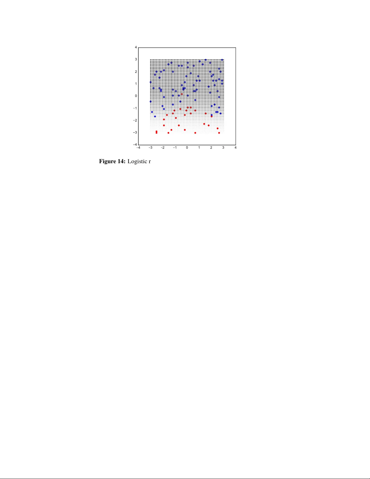
Edw ard: A librar y f or probabilis tic modeling, inf erence, and cr iticism Dustin T ran, Alp Kucuk elbir , A dji B. Dieng, Ma ja R udolph, Da wen Liang, and Da vid M. Blei Columbia Univ ersity February 2, 2017 Abstract Probabilistic modeling is a po werful approach f or analyzing empirical information. W e de- scribe Edwar d , a library f or probabilistic modeling. Edward’ s design reﬂects an iterativ e process pioneered b y George Box: build a model of a phenomenon, make inferences about the model giv en data, and criticize the model’ s ﬁt to the data. Edward suppor ts a broad class of probabilistic models, eﬃcient algorithms for inference, and many techniques for model cr iticism. The library builds on top of T ensorFlow to suppor t distributed training and hardware such as GPUs. Edward enables the dev elopment of complex probabilistic models and their algor ithms at a massiv e scale. Keyw ords: Probabilistic Models; Bay esian Inference; Model Criticism; Neural Netw orks; Scalable Computation; Probabilistic Programming. 1 Contents 1 Introduction 1 2 Getting Started 3 3 Design 5 3.1 Data . . . . . . . . . . . . . . . . . . . . . . . . . . . . . . . . . . . . . . . . . . 5 3.2 Models . . . . . . . . . . . . . . . . . . . . . . . . . . . . . . . . . . . . . . . . 6 3.3 Inf erence . . . . . . . . . . . . . . . . . . . . . . . . . . . . . . . . . . . . . . . 10 3.4 Criticism . . . . . . . . . . . . . . . . . . . . . . . . . . . . . . . . . . . . . . . 18 4 End-to-end Examples 21 4.1 Ba yesian Linear Regression . . . . . . . . . . . . . . . . . . . . . . . . . . . . . . 21 4.2 Logistic and N eural Netw ork Classiﬁcation . . . . . . . . . . . . . . . . . . . . . 23 5 A ckno wledgments 28 1 Details in this paper descr ibe Edward version 1.2.1, released Jan 30, 2017. 1 Introduction Probabilistic modeling is a pow er ful approach for analyzing empir ical inf or mation ( T uk e y , 1962 ; Ne well and Simon , 1976 ; Bo x , 1976 ). Probabilistic models are essential to ﬁelds related to its methodology , such as statistics ( Friedman et al. , 2001 ; Gelman et al. , 2013 ) and machine learning ( Murphy , 2012 ; Goodf ellow et al. , 2016 ), as well as ﬁelds related to its application, such as com- putational biology ( Friedman et al. , 2000 ), computational neuroscience ( Day an and Abbott , 2001 ), cognitiv e science ( T enenbaum et al. , 2011 ), information theory ( MacKay , 2003 ), and natural lan- guage processing ( Manning and Schütze , 1999 ). Software sys tems for probabilistic modeling pro vide new and faster wa ys of experimentation. This enables researc h adv ances in probabilistic modeling that could not ha v e been completed before. As an ex ample of such software sys tems, w e point to earl y w ork in ar tiﬁcial intelligence. Expert sys tems were designed from human expertise, which in tur n enabled larger reasoning steps according to exis ting know ledge ( Buchanan et al. , 1969 ; Minsky , 1975 ). With connectionist models, the design f ocused on neuron-like processing units, which learn from e xper ience; this drov e new applications of ar tiﬁcial intellig ence ( Hopﬁeld , 1982 ; R umelhar t et al. , 1988 ). As another ex ample, w e point to earl y work in statis tical computing, where interest g re w broadly out of eﬃcient computation f or problems in statis tical anal ysis. The S language, dev eloped b y John Chambers and colleagues at Bell Laboratories ( Beck er and Chambers , 1984 ; Chambers and Hastie , 1992 ), f ocused on an interactiv e environment f or data analy sis, with simple y et r ich syntax to quic kly turn ideas into software. It is a predecessor to the R language ( Ihaka and Gentleman , 1996 ). More targ eted environments such as BUGS ( Spiegelhalter et al. , 1995 ), which f ocuses on Bay esian analy sis of statis tical models, helped launch the emerging ﬁeld of probabilistic programming. W e are motivated to build on these earl y works in probabilistic systems—where in modern applica- tions, ne w challeng es ar ise in their design and implementation. W e highlight two challeng es. First, statis tics and machine lear ning hav e made signiﬁcant advances in the methodology of probabilis- tic models and their inference (e.g., Hoﬀman et al. ( 2013 ); Ranganath et al. ( 2014 ); Rezende et al. ( 2014 )). For softw are systems to enable fas t e xper imentation, we require r ich abstractions that can capture these advances: it must encompass both a broad class of probabilistic models and a broad class of algor ithms f or their eﬃcient inference. Second, researchers are increasingly motivated to emplo y complex probabilistic models and at an un precedented scale of massiv e data ( Bengio et al. , 2013 ; Ghahramani , 2015 ; Lake et al. , 2016 ). Thus w e require an eﬃcient computing environment that suppor ts distributed training and integ ration of hardware such as (multiple) GPUs. W e present Edw ard , a probabilistic modeling library named after the statis tician Geor ge Edward Pelham Bo x. Edward is built around an iterative process for probabilistic modeling, pioneered by Bo x and his collaborators ( Bo x and Hunter , 1962 , 1965 ; Bo x and Hill , 1967 ; Box , 1976 , 1980 ). The process is as f ollo ws: given data from some unkno wn phenomena, ﬁrst, f ormulate a model of the phenomena; second, use an algor ithm to infer the model’ s hidden structure, thus reasoning about the phenomena; third, cr iticize ho w w ell the model captures the data ’ s generativ e process. As w e criticize our model’ s ﬁt to the data, we revise components of the model and repeat to form an iterativ e loop ( Bo x , 1976 ; Blei , 2014 ; Gelman et al. , 2013 ). Edward builds infrastructure to enable this loop: 1. For modeling , Edward pro vides a language of random variables to construct a broad class of models: directed g raphical models ( Pear l , 1988 ), stoc hastic neural networks ( Neal , 1990 ), and programs with stochas tic control ﬂo w ( Goodman et al. , 2012 ). 2. For inf erence , Edward pro vides algor ithms such as stochas tic and black bo x v ar iational infer - ence ( Hoﬀman et al. , 2013 ; Ranganath et al. , 2014 ), Hamiltonian Monte Carlo ( Neal , 1993 ), and stochas tic g radient Lange vin dynamics ( W elling and T eh , 2011 ). Edw ard also provides infrastructure to make it easy to dev elop ne w algor ithms. 1 3. For criticism , Edw ard provides methods from scoring rules ( W inkler , 1996 ) and predictiv e chec ks ( Box , 1980 ; Rubin , 1984 ). Edward is built on top of T ensorFlo w , a library for numer ical computing using data ﬂow g raphs ( Abadi et al. , 2016 ). T ensorFlo w enables Edward to speed up computation with hardware such as GPUs, to scale up computation with distributed training, and to simplify engineer ing eﬀor t with automatic diﬀerentiation. In Section 2 , w e demonstrate Edward with an e xample. In Section 3 , w e describe the design of Edward. In Section 4 , we provide ex amples of ho w standard tasks in statis tics and machine lear ning can be solv ed with Edward. Related w ork Probabilistic programming. There has been much work on programming languages which spec- ify broad classes of probabilistic models, or probabilistic programs. R ecent works include Church ( Goodman et al. , 2012 ), V enture ( Mansinghka et al. , 2014 ), Anglican ( W ood et al. , 2015 ), Stan ( Car - penter et al. , 2016 ), and W ebPPL ( Goodman and Stuhlmüller , 2014 ). The most impor tant distinction in Edward stems from motivation. W e are interested in deplo ying probabilistic models to man y real w orld applications, ranging from the size of data and data structure, suc h as large text cor pora or man y br ief audio signals, to the size of model and class of models, such as small nonparametric models or deep generativ e models. Thus Edward is built with fas t computation in mind. Black box inference. Black box algor ithms are typically based on Monte Carlo methods, and make v er y fe w assumptions about the model ( Metropolis and Ulam , 1949 ; Has tings , 1970 ; Geman and Geman , 1984 ). Our motivation as outlined abo v e presents a new set of challeng es in both inf erence research and software design. As a ﬁrst consequence, w e f ocus on v ar iational inference ( Hinton and van Camp , 1993 ; W aterhouse et al. , 1996 ; Jordan et al. , 1999 ). As a second consequence, we encourage active research on inference b y providing a class hierarch y of inference algor ithms. As a third consequence, our inf erence algorithms aim to take advantag e of as much structure as possible from the model. Edward supports all types of inf erence, whether they be black bo x or model-speciﬁc ( Dempster et al. , 1977 ; Hoﬀman et al. , 2013 ). Computational frame w orks. There are man y computational frame works, pr imar il y built f or deep learning: as of this date, this includes T ensorFlo w ( Abadi et al. , 2016 ), Theano ( Al-Rf ou et al. , 2016 ), T orc h ( Collobert and Kavukcuoglu , 2011 ), neon ( Nervana Systems , 2014 ), and the Stan Math Library ( Carpenter et al. , 2015 ). These are incredible tools which Edward emplo ys as a back end. In ter ms of abstraction, Edward sits one lev el higher . High-le vel deep learning libraries. N eural netw ork libraries such as K eras ( Chollet , 2015 ) and Lasagne ( Dieleman et al. , 2015 ) are at a similar abstraction lev el as Edward. How ev er both are pr i- marily interested in parameterizing complicated functions f or supervised lear ning on large datasets. W e are interested in probabilistic models which apply to a wide ar ra y of lear ning tasks. These tasks ma y hav e both complicated likelihood and complicated priors (neural netw orks are an option but not a necessity). Theref ore our goals are or thogonal and in f act mutually beneﬁcial to each other . F or e xample, we use Keras ’ abstraction as a wa y to easily specify models parameterized b y deep neural netw orks. 2 2 Getting Started Probabilistic modeling in Edward uses a simple language of random variables. Here we will sho w a Ba yesian neural network. It is a neural netw ork with a prior distr ibution on its weights. Firs t, simulate a to y dataset of 50 observations with a cosine relationship. 1 import numpy as np 2 3 x_train = np.linspace(-3, 3, num=50) 4 y_train = np.cos(x_train) + np.random.normal(0, 0.1, size=50) 5 x_train = x_train.astype(np.float32).reshape((50, 1)) 6 y_train = y_train.astype(np.float32).reshape((50, 1)) 4 2 0 2 4 2.0 1.5 1.0 0.5 0.0 0.5 1.0 1.5 2.0 (x, y) Figure 1: Simulated data with a cosine relationship between x and y . Ne xt, deﬁne a tw o-lay er Ba y esian neural netw ork. Here, w e deﬁne the neural netw ork manually with tanh nonlinearities. 1 import tensorflow as tf 2 from edward.models import Normal 3 4 W_0 = Normal (mu=tf.zeros([1, 2]), sigma=tf.ones([1, 2])) 5 W_1 = Normal (mu=tf.zeros([2, 1]), sigma=tf.ones([2, 1])) 6 b_0 = Normal (mu=tf.zeros(2), sigma=tf.ones(2)) 7 b_1 = Normal (mu=tf.zeros(1), sigma=tf.ones(1)) 8 9 x = x_train 10 y = Normal (mu=tf.matmul(tf.tanh(tf.matmul(x, W_0) + b_0), W_1) + b_1, 11 sigma=0.1) Ne xt, make inferences about the model from data. W e will use v ar iational inference. Specify a normal approximation o v er the weights and biases. 1 qW_0 = Normal (mu=tf.Variable(tf.zeros([1, 2])), 2 sigma=tf.nn.softplus(tf.Variable(tf.zeros([1, 2])))) 3 qW_1 = Normal (mu=tf.Variable(tf.zeros([2, 1])), 4 sigma=tf.nn.softplus(tf.Variable(tf.zeros([2, 1])))) 5 qb_0 = Normal (mu=tf.Variable(tf.zeros(2)), 6 sigma=tf.nn.softplus(tf.Variable(tf.zeros(2)))) 7 qb_1 = Normal (mu=tf.Variable(tf.zeros(1)), 8 sigma=tf.nn.softplus(tf.Variable(tf.zeros(1)))) Deﬁning tf.Variable allo ws the variational factors ’ parameters to vary . They are all initialized at 0. The standard deviation parameters are constrained to be greater than zero according to a softplus transf ormation 2 . No w , run variational inference with the Kullbac k -Leibler diver gence in order to infer the model’ s latent variables giv en data. W e specify 1000 iterations. 2 The softplus function is deﬁned as softplus ( x ) = log(1 + exp( x )) . 3 1 import edward as ed 2 3 inference = ed. KLqp ({W_0: qW_0, b_0: qb_0, 4 W_1: qW_1, b_1: qb_1}, data={y: y_train}) 5 inference.run(n_iter=1000) Finall y , cr iticize the model ﬁt. Ba yesian neural netw orks deﬁne a distribution o ver neural netw orks, so w e can perf or m a g raphical c heck. Draw neural networks from the inf er red model and visualize ho w well it ﬁts the data. 4 2 0 2 4 2.0 1.5 1.0 0.5 0.0 0.5 1.0 1.5 2.0 (x, y) posterior draws Figure 2: Posterior dra ws from the inf er red Bay esian neural network. The model has captured the cosine relationship betw een x and y in the obser v ed domain. 4 3 Design Edward’ s design reﬂects the building blocks f or probabilistic modeling. It deﬁnes interchang eable components, enabling rapid experimentation and research with probabilistic models. Edward is named after the inno vativ e statistician Georg e Edward Pelham Bo x. Edward f ollo ws Bo x’ s philosoph y of statistics and machine lear ning ( Box , 1976 ). Firs t g ather data from some real-w orld phenomena. Then cycle through Box’ s loop ( Blei , 2014 ). 1. Build a probabilistic model of the phenomena. 2. Reason about the phenomena given model and data. 3. Criticize the model, re vise and repeat. Model Inf er Data Criticize Figure 3: Box’ s loop. Here ’ s a toy ex ample. A child ﬂips a coin ten times, with the set of outcomes being [0, 1, 0, 0 , 0, 0, 0, 0, 0, 1] , where 0 denotes tails and 1 denotes heads. She is interested in the probability that the coin lands heads. T o analyze this, she ﬁrst builds a model: suppose she assumes the coin ﬂips are independent and land heads with the same probability . Second, she reasons about the phenomenon: she infers the model’ s hidden structure given data. F inally , she cr iticizes the model: she analyzes whether her model captures the real-w orld phenomenon of coin ﬂips. If it doesn ’ t, then she ma y re vise the model and repeat. W e describe modules enabling this analy sis. 3.1 Data Data deﬁnes a set of obser vations. There are three wa ys to read data in Edward. Preloaded dat a. A cons tant or variable in the T ensorFlo w g raph holds all the data. This setting is the fas test to w ork with and is recommended if the data ﬁts in memor y . Represent the data as NumPy ar ra ys or T ensorFlo w tensors. 1 x_data = np.array([0, 1, 0, 0, 0, 0, 0, 0, 0, 1]) 2 x_data = tf.constant([0, 1, 0, 0, 0, 0, 0, 0, 0, 1]) During inference, we store them in T ensorFlo w variables internally to prev ent copying data more than once in memor y . F eeding. Manual code provides the data when running each step of inference. This setting pro vides the most ﬁne control which is useful f or e xper imentation. 5 Represent the data as T ensorFlo w placeholders, which are nodes in the graph that are fed at run- time. 1 x_data = tf.placeholder(tf.float32, [100, 25]) # placeholder of shape (100, 25) During inference, the user must manually feed the placeholders. At each step, call inference.update() while passing in a feed_dict dictionar y which binds placeholders to realized values as an argument. If the values do not chang e ov er inf erence updates, one can also bind the placeholder to values within the data argument when ﬁrst constr ucting inf erence. Reading from ﬁles. An input pipeline reads the data from ﬁles at the beginning of a T ensorFlo w graph. This setting is recommended if the data does not ﬁt in memor y . 1 filename_queue = tf.train.string_input_producer(...) 2 reader = tf.SomeReader() 3 ... Represent the data as T ensorFlo w tensors, where the tensors are the output of data readers. Dur ing inf erence, each update will be automatically e valuated o v er new batch tensors represented through the data readers. 3.2 Models A probabilistic model is a joint distribution p ( x , z ) of data x and latent v ar iables z . In Edward, w e specify models using a simple language of random variables. A random variable x is an object parameter ized b y tensors θ ∗ , where the number of random variables in one object is determined by the dimensions of its parameters. 1 from edward.models import Normal , Exponential 2 3 # univariate normal 4 Normal (mu=tf.constant(0.0), sigma=tf.constant(1.0)) 5 # vector of 5 univariate normals 6 Normal (mu=tf.zeros(5), sigma=tf.ones(5)) 7 # 2 x 3 matrix of Exponentials 8 Exponential (lam=tf.ones([2, 3])) For multivariate distr ibutions, the multivariate dimension is the inner most (r ight-most) dimension of the parameters. 1 from edward.models import Dirichlet , MultivariateNormalFull 2 3 # K-dimensional Dirichlet 4 Dirichlet (alpha=tf.constant([0.1] * K) 5 # vector of 5 K-dimensional multivariate normals 6 MultivariateNormalFull (mu=tf.zeros([5, K]), sigma=...) 7 # 2 x 5 matrix of K-dimensional multivariate normals 8 MultivariateNormalFull (mu=tf.zeros([2, 5, K]), sigma=...) Random v ar iables are equipped with methods such as log_prob() , log p ( x | θ ∗ ) , mean() , E p ( x | θ ∗ ) [ x ] , and sample() , x ∗ ∼ p ( x | θ ∗ ) . Further , each random variable is associated to a tensor x ∗ in the computational graph, which represents a single sample x ∗ ∼ p ( x | θ ∗ ) . This mak es it easy to parameterize random v ar iables with complex deter ministic s tr ucture, such as with deep neural netw orks, a div erse set of math operations, and compatibility with third par ty libraries which also build on T ensorFlo w . The design also enables compositions of random variables to capture comple x stochastic structure. They operate on x ∗ . 1 from edward.models import Normal 2 3 x = Normal (mu=tf.zeros(10), sigma=tf.ones(10)) 4 y = tf.constant(5.0) 5 x + y, x - y, x * y, x / y 6 tf.tanh(x * y) 7 tf.gather(x, 2) # 3rd normal rv in the vector 6 x x ∗ y x ∗ + y Figure 4: Random variables can be combined with other T ensorFlo w ops. Belo w we descr ibe ho w to build models b y composing random variables. For a list of random v ar iables supported in Edward, see the T ensorFlo w distributions API. 3 Edward random variables build on top of them, inheriting the same arguments and class methods. A dditional methods are also av ailable, detailed in Edward’ s API. Composing Random V ariables Core to Edw ard’ s design is compositionality . Compositionality enables ﬁne control of modeling, where models are represented as a collection of random variables. W e outline how to write popular classes of models using Edward: directed graphical models, neural netw orks, Bay esian nonparametr ics, and probabilistic prog rams. Directed Graphical Models Graphical models are a r ich f ormalism for specifying probability distributions ( Koller and Friedman , 2009 ). In Edward, directed edges in a g raphical model are implicitly deﬁned when random v ar iables are composed with one another . W e illustrate with a Beta-Ber noulli model, p ( x , θ ) = Beta ( θ | 1 , 1) 50 Y n =1 Bernoulli ( x n | θ ) , where θ is a latent probability shared across the 50 data points x ∈ { 0 , 1 } 50 . 1 from edward.models import Bernoulli , Beta 2 3 theta = Beta (a=1.0, b=1.0) 4 x = Bernoulli (p=tf.ones(50) * theta) θ θ ∗ tf.ones(50) x x ∗ Figure 5: Computational g raph f or a Beta-Ber noulli program. The random variable x ( x ) is 50-dimensional, parameterized b y the random tensor θ ∗ . Fetching the object x.value() ( x ∗ ) from session runs the g raph: it simulates from the g enerative process and outputs a binar y v ector of 50 elements. With computational graphs, it is also natural to build mutable states within the probabilistic program. As a typical use of computational graphs, such states can deﬁne model parameters, that is, parameters that we will alwa ys compute point estimates f or and not be uncer tain about. In T ensorFlo w , this is giv en by a tf.Variable . 3 https://www.tensorflow.org/versions/master/api_docs/python/contrib.distributions.html 7 1 from edward.models import Bernoulli 2 3 theta = tf.Variable(0.0) 4 x = Bernoulli (p=tf.ones(50) * tf.sigmoid(theta)) Another use case of mutable states is f or building discr iminativ e models p ( y | x ) , where x are f eatures that are input as training or test data . The program can be written independent of the data, using a mutable state ( tf.placeholder ) f or x in its graph. Dur ing training and testing, w e f eed the placeholder the appropr iate v alues. Neural Netw orks As Edward uses T ensorFlo w , it is easy to construct neural netw orks f or probabilistic modeling ( Rumel- hart et al. , 1988 ). For ex ample, one can specify stoc hastic neural netw orks ( Neal , 1990 ). High-lev el libraries such as Keras 4 and T ensorFlo w Slim 5 can be used to easily construct deep neural netw orks. W e illustrate this with a deep generativ e model ov er binary data { x n } ∈ { 0 , 1 } N × 28 ∗ 28 . z n x n θ N Figure 6: Graphical representation of a deep generativ e model. The model speciﬁes a generativ e process where f or each n = 1 , . . . , N , z n ∼ Normal ( z n | 0 , I ) , x n | z n ∼ Bernoulli ( x n | p = NN( z n ; θ )) . The latent space is z n ∈ R d and the likelihood is parameterized b y a neural netw ork NN with parameters θ . W e will use a tw o-lay er neural netw ork with a fully connected hidden lay er of 256 units (with R eLU activation) and whose output is 28 ∗ 28 -dimensional. The output will be unconstrained, parameterizing the logits of the Ber noulli likelihood. With T ensorFlo w Slim, we write this model as f ollo ws: 1 from edward.models import Bernoulli , Normal 2 from tensorflow.contrib import slim 3 4 z = Normal (mu=tf.zeros([N, d]), sigma=tf.ones([N, d])) 5 h = slim.fully_connected(z, 256) 6 x = Bernoulli (logits=slim.fully_connected(h, 28 * 28, activation_fn=None)) With Keras, we wr ite this model as follo ws: 1 from edward.models import Bernoulli , Normal 2 from keras.layers import Dense 3 4 z = Normal (mu=tf.zeros([N, d]), sigma=tf.ones([N, d])) 5 h = Dense(256, activation= ’relu’ )(z.value()) 6 x = Bernoulli (logits=Dense(28 * 28)(h)) Keras and T ensorFlo w Slim automatically manage T ensorFlo w variables, which ser v e as parameters of the high-lev el neural netw ork la yers. This sav es the trouble of having to manag e them manuall y . Ho we ver , note that neural network parameters deﬁned this wa y alwa ys serve as model parameters. That is, the parameters are not exposed to the user so we cannot be Ba yesian about them with pr ior distributions. 4 http://keras.io 5 https://github.com/tensorflow/tensorflow/tree/master/tensorflow/contrib/slim 8 Ba yesian Nonparametrics Ba yesian nonparametr ics enable rich probability models by working o v er an inﬁnite-dimensional parameter space ( Hjor t et al. , 2010 ). Edw ard suppor ts the tw o typical approaches to handling these models: collapsing the inﬁnite-dimensional space and lazily deﬁning the inﬁnite-dimensional space. For the collapsed approach, see the Gaussian process classiﬁcation tutorial as an example. W e spec- ify distributions o v er the function ev aluations of the Gaussian process, and the Gaussian process is implicitly marginalized out. This approach is also useful f or Poisson process models. T o w ork directly on the inﬁnite-dimensional space, one can lev erage random variables with control ﬂo w operations in T ensorFlo w . At r untime, the control ﬂow will lazil y deﬁne an y parameters in the space necessar y in order to generate samples. As an ex ample, we use a while loop to deﬁne a Dirichlet process according to its stic k breaking representation. Probabilistic Programs Probabilistic programs greatly e xpand the scope of probabilistic models ( Goodman et al. , 2012 ). For - mally , Edw ard is a T uring-complete probabilistic programming language. This means that Edward can represent any computable probability distr ibution. p p ∗ tf.while_loop(...) a ∗ a x x ∗ Figure 7: Computational g raph f or a probabilistic program with stochastic control ﬂow . Random variables can be composed with control ﬂo w operations, enabling probabilistic prog rams with stoc hastic control ﬂow . Stoc hastic control ﬂo w deﬁnes dynamic conditional dependencies, kno wn in the literature as contingent or exis tential dependencies ( Mansinghka et al. , 2014 ; Wu et al. , 2016 ). See abo v e, where x may or ma y not depend on a f or a given ex ecution. Stoc hastic control ﬂow produces diﬃculties f or algorithms that le v erage the graph structure; the relationship of conditional dependencies chang es across ex ecution traces. Impor tantly , the computa- tional g raph pro vides an elegant wa y of teasing out static conditional dependence structure ( p ) from dynamic dependence structure ( a ) . W e can perform model parallelism ov er the static structure with GPUs and batch training, and use generic computations to handle the dynamic structure. De v eloping Custom Random V ariables Oftentimes we ’ d like to implement our o wn random variables. T o do so, wr ite a class that inherits the RandomVariable class in edward.models and the Distribution class in tf.contrib.distributions (in that order). A template is provided below . 1 from edward.models import RandomVariable 2 from tensorflow.contrib.distributions import Distribution 3 4 class CustomRandomVariable( RandomVariable , Distribution ): 5 def __init__ (self, *args, **kwargs): 6 super(CustomRandomVariable, self). __init__ (*args, **kwargs) 7 8 def _log_prob(self, value): 9 raise NotImplementedError( "log_prob is not implemented" ) 10 11 def _sample_n(self, n, seed=None): 12 raise NotImplementedError( "sample_n is not implemented" ) 9 One method that all Edw ard random variables call dur ing instantiation is _sample_n() . It takes an in- teger n as input and outputs a tensor of shape (n,) + batch_shape + event_shape . T o implement it, y ou can f or e xample wrap a NumPy/SciPy function inside the T ensorFlow operation tf.py_func() . For other methods and attr ibutes one can implement, see the API documentation in T ensorFlow’ s Distribution class. A dvanced settings Sometimes the random variable y ou ’ d like to w ork with already exis ts in Edward, but it is missing a par ticular f eature. One hack is to implement and ov er write the missing method. For e xample, to implement y our own sampling for Poisson : 1 import edward as ed 2 from edward.models import Poisson 3 from scipy.stats import poisson 4 5 def _sample_n(self, n=1, seed=None): 6 # define Python function which returns samples as a Numpy array 7 def np_sample(lam, n): 8 return poisson.rvs(mu=lam, size=n, random_state=seed).astype(np.float32) 9 10 # wrap python function as tensorflow op 11 val = tf.py_func(np_sample, [self.lam, n], [tf.float32])[0] 12 # set shape fr om unknown shape 13 batch_event_shape = self.get_batch_shape().concatenate(self.get_event_shape()) 14 shape = tf.concat([tf.expand_dims(n, 0), 15 tf.constant(batch_event_shape.as_list(), dtype=tf.int32)], 16 0) 17 val = tf.reshape(val, shape) 18 return val 19 20 Poisson._sample_n = _sample_n 21 22 sess = ed. get_session () 23 x = Poisson(lam=1.0) 24 sess.run(x.value()) 25 ## 1.0 26 sess.run(x.value()) 27 ## 4.0 (Note the function np_sample should broadcast cor rectly if you ’ d like to work with non-scalar param- eters; it is not cor rect in this toy implementation.) Sometimes the random variable you ’ d like to work with does not ev en admit (easy) sampling, and y ou ’ re only using it as a likelihood “node ” rather than as some pr ior to parameters of another random variable. Y ou can a void ha ving to implement _sample_n altog ether: after creating CustomRandomVariable , instantiate it with the value argument: 1 x = CustomRandomVariable(custom_params=params, value=tf.zeros_like(params)) This ﬁx es the associated value of the random variable to a bunch of zeros and av oids the _sample_n error that appears other wise. Mak e sure that the value matches the desired shape of the random variable. 3.3 Inf erence W e describe how to per f or m inf erence in probabilistic models. Suppose we hav e a model p ( x , z , β ) of data x train with latent v ar iables ( z , β ) . Consider the posterior inf erence problem, q ( z , β ) ≈ p ( z , β | x train ) , in whic h the task is to appro ximate the poster ior p ( z , β | x train ) using a f amily of distributions, q ( z , β ; λ ) , inde x ed by parameters λ . 10 In Edw ard, let z and beta be latent variables in the model, where w e observe the random v ar iable x with data x_train . Let qz and qbeta be random v ar iables deﬁned to approximate the posterior . W e write this problem as f ollo ws: 1 inference = ed. Inference ({z: qz, beta: qbeta}, {x: x_train}) Inference is an abstract class which takes two inputs. The ﬁrst is a collection of latent random v ar i- ables beta and z , along with “posterior v ar iables ” qbeta and qz , which are associated to their respective latent variables. The second is a collection of obser v ed random v ar iables x , which is associated to the data x_train . Inf erence adjusts parameters of the distribution of qbeta and qz to be close to the posterior p ( z , β | x train ) . Running inference is as simple as running one method. 1 inference = ed. Inference ({z: qz, beta: qbeta}, {x: x_train}) 2 inference.run() Inf erence also suppor ts ﬁne control of the training procedure. 1 inference = ed. Inference ({z: qz, beta: qbeta}, {x: x_train}) 2 inference.initialize() 3 4 tf.global_variables_initializer().run() 5 6 for _ in range(inference.n_iter): 7 info_dict = inference.update() 8 inference.print_progress(info_dict) 9 10 inference.finalize() initialize() builds the algor ithm’ s update rules (computational g raph) f or λ ; tf.global_variables_initializer().run() initializes λ (T ensorFlow variables in the graph); update() runs the graph once to update λ , which is called in a loop until conv ergence; finalize() r uns any computation as the algor ithm terminates. The run() method is a simple wrapper f or this procedure. Other Settings W e highlight other settings dur ing inf erence. Model parameters . Model parameters are parameters in a model that w e will alwa ys compute point estimates f or and not be uncertain about. The y are deﬁned with tf.Variable s, where the inference problem is ˆ θ ← optimize p ( x train ; θ ) 1 from edward.models import Normal 2 3 theta = tf.Variable(0.0) 4 x = Normal (mu=tf.ones(10) * theta, sigma=1.0) 5 6 inference = ed. Inference ({}, {x: x_train}) Only a subset of inf erence algor ithms support estimation of model parameters. (Note also that this inf erence example does not hav e any latent variables. It is only about estimating theta given that w e observe x = x train . W e can add them so that inf erence is both posterior inf erence and parameter estimation.) For e xample, model parameters are useful when appl ying neural netw orks from high-le vel libraries such as Keras and T ensorFlo w Slim. See the model compositionality subsection f or more details. 11 Conditional infer ence . In conditional inf erence, only a subset of the posterior is inf er red while the rest are ﬁx ed using other inferences. The inf erence problem is q ( β ) q ( z ) ≈ p ( z , β | x train ) where parameters in q ( β ) are estimated and q ( z ) is ﬁxed. In Edward, we enable conditioning by binding random variables to other random variables in data . 1 inference = ed. Inference ({beta: qbeta}, {x: x_train, z: qz}) In the inf erence compositionality subsection, we descr ibe ho w to construct inf erence by composing man y conditional inference algor ithms. Implicit prior samples . Latent variables can be deﬁned in the model without any posterior inf er - ence o v er them. They are implicitly marginalized out with a single sample. The inf erence problem is q ( β ) ≈ p ( β | x train , z ∗ ) where z ∗ ∼ p ( z | β ) is a prior sample. 1 inference = ed. Inference ({beta: qbeta}, {x: x_train}) For e xample, implicit prior samples are useful for g enerative adv ersar ial netw orks. Their infer - ence problem does not require an y inf erence o ver the latent v ariables; it uses samples from the prior . Classes of Inf erence Inf erence is broadly classiﬁed under three classes: v ar iational inference, Monte Carlo, and ex act inf erence. W e highlight how to use inference algor ithms from each class. As an example, we assume a mixture model with latent mixture assignments z , latent cluster means beta , and obser v ations x : p ( x , z , β ) = Normal ( x | β z , I ) Categor ical ( z | π ) Normal ( β | 0 , I ) . V ariational Infer ence In variational inf erence, the idea is to posit a famil y of appro ximating distr ibutions and to ﬁnd the closest member in the famil y to the posterior ( Jordan et al. , 1999 ). W e wr ite an approximating fam- ily , q ( β ; µ, σ ) = Normal ( β ; µ, σ ) , q ( z ; π ) = Categor ical ( z ; π ) , using T ensorFlow variables to represent its parameters λ = { π , µ, σ } . 1 from edward.models import Categorical , Normal 2 3 qbeta = Normal (mu=tf.Variable(tf.zeros([K, D])), 4 sigma=tf.exp(tf.Variable(tf.zeros[K, D]))) 5 qz = Categorical (logits=tf.Variable(tf.zeros[N, K])) 6 7 inference = ed. VariationalInference ({beta: qbeta, z: qz}, data={x: x_train}) Giv en an objectiv e function, variational inf erence optimizes the famil y with respect to tf.Variable s. Speciﬁc v ar iational inference algor ithms inher it from the VariationalInference class to deﬁne their o wn methods, such as a loss function and g radient. For ex ample, we represent MAP estimation with an approximating famil y ( qbeta and qz ) of PointMass random variables, i.e., with all probability mass concentrated at a point. 12 1 from edward.models import PointMass 2 3 qbeta = PointMass (params=tf.Variable(tf.zeros([K, D]))) 4 qz = PointMass (params=tf.Variable(tf.zeros(N))) 5 6 inference = ed. MAP ({beta: qbeta, z: qz}, data={x: x_train}) MAP inher its from VariationalInference and deﬁnes a loss function and update r ules; it uses e xisting optimizers inside T ensorFlow . Monte Carlo Monte Car lo appro ximates the posterior using samples ( R ober t and Casella , 1999 ). Monte Carlo is an inf erence where the appro ximating f amily is an empirical distribution, q ( β ; { β ( t ) } ) = 1 T T X t =1 δ ( β , β ( t ) ) , q ( z ; { z ( t ) } ) = 1 T T X t =1 δ ( z , z ( t ) ) . The parameters are λ = { β ( t ) , z ( t ) } . 1 from edward.models import Empirical 2 3 T = 10000 # number of samples 4 qbeta = Empirical (params=tf.Variable(tf.zeros([T, K, D])) 5 qz = Empirical (params=tf.Variable(tf.zeros([T, N])) 6 7 inference = ed. MonteCarlo ({beta: qbeta, z: qz}, data={x: x_train}) Monte Carlo algor ithms proceed by updating one sample β ( t ) , z ( t ) at a time in the empir ical approxi- mation. Monte Carlo algor ithms proceed by updating one sample β ( t ) , z ( t ) at a time in the empir ical appro ximation. Marko v chain Monte Carlo does this sequentially to update the cur rent sample (inde x t of tf.Variable s) conditional on the last sample (index t − 1 of tf.Variable s). Speciﬁc Monte Carlo samplers deter mine the update rules; they can use gradients such as in Hamiltonian Monte Carlo ( Neal , 2011 ) and graph structure such as in sequential Monte Carlo ( Doucet et al. , 2001 ). Exact Inf erence This approach also e xtends to algorithms that usually require tedious algebraic manipulation. With symbolic algebra on the nodes of the computational graph, w e can unco ver conjugacy relationships betw een random variables. Users can then integrate out variables to automaticall y derive classical Gibbs ( Gelfand and Smith , 1990 ), mean-ﬁeld updates ( Bishop , 2006 ), and ex act inference. Composing Inf erences Core to Edward’ s design is compositionality . Compositionality enables ﬁne control of inference, where w e can write inference as a collection of separate inf erence programs. W e outline how to wr ite popular classes of compositional inferences using Edward: h ybr id algo- rithms and messag e passing algor ithms. W e use the r unning ex ample of a mixture model with latent mixture assignments z , latent cluster means beta , and obser vations x . 13 Hybrid algorithms Hybrid algorithms lev erage diﬀerent inferences for each latent variable in the posterior . As an exam- ple, we demonstrate variational EM, with an appro ximate E-step ov er local v ar iables and an M-s tep o v er global v ar iables. W e alter nate with one update of each ( Neal and Hinton , 1993 ). 1 from edward.models import Categorical , PointMass 2 3 qbeta = PointMass (params=tf.Variable(tf.zeros([K, D]))) 4 qz = Categorical (logits=tf.Variable(tf.zeros[N, K])) 5 6 inference_e = ed. VariationalInference ({z: qz}, data={x: x_data, beta: qbeta}) 7 inference_m = ed. MAP ({beta: qbeta}, data={x: x_data, z: qz}) 8 ... 9 for _ in range(10000): 10 inference_e.update() 11 inference_m.update() In data , we include bindings of prior latent variables ( z or beta ) to posterior latent variables ( qz or qbeta ). This per f or ms conditional inference, where only a subset of the posterior is inferred while the rest are ﬁx ed using other inferences. This extends to many algorithms: f or example, ex act EM f or e xponential families; contrastiv e di- v erg ence ( Hinton , 2002 ); pseudo-marginal and ABC methods ( Andr ieu and Roberts , 2009 ); Gibbs sampling within variational inference ( W ang and Blei , 2012 ); Laplace variational inference ( W ang and Blei , 2013 ); and structured v ar iational auto-encoders ( Johnson et al. , 2016 ). Message passing algorithms Message passing algor ithms operate on the posterior distribution using a collection of local inferences ( K oller and Fr iedman , 2009 ). As an e xample, we demonstrate expectation propagation. W e split a mixture model to be ov er two random variables x1 and x2 along with their latent mixture assignments z1 and z2 . 1 from edward.models import Categorical , Normal 2 3 N1 = 1000 # number of data points in first data set 4 N2 = 2000 # number of data points in second data set 5 D = 2 # data dimension 6 K = 5 # number of clusters 7 8 # MODEL 9 beta = Normal (mu=tf.zeros([K, D]), sigma=tf.ones([K, D])) 10 z1 = Categorical (logits=tf.zeros([N1, K])) 11 z2 = Categorical (logits=tf.zeros([N2, K])) 12 x1 = Normal (mu=tf.gather(beta, z1), sigma=tf.ones([N1, D])) 13 x2 = Normal (mu=tf.gather(beta, z2), sigma=tf.ones([N2, D])) 14 15 # INFERENCE 16 qbeta = Normal (mu=tf.Variable(tf.zeros([K, D])), 17 sigma=tf.nn.softplus(tf.Variable(tf.zeros([K, D])))) 18 qz1 = Categorical (logits=tf.Variable(tf.zeros[N1, K])) 19 qz2 = Categorical (logits=tf.Variable(tf.zeros[N2, K])) 20 21 inference_z1 = ed. KLpq ({beta: qbeta, z1: qz1}, {x1: x1_train}) 22 inference_z2 = ed. KLpq ({beta: qbeta, z2: qz2}, {x2: x2_train}) 23 ... 24 for _ in r ange(10000): 25 inference_z1.update() 26 inference_z2.update() W e alter nate updates for each local inf erence, where the global posterior factor q ( β ) is shared across both inf erences ( Gelman et al. , 2014 ). With T ensorFlo w’ s distributed training, compositionality enables distributed message passing o ver a cluster with many work ers. The computation can be fur ther sped up with the use of GPUs via data and model parallelism. 14 This e xtends to many algorithms: f or example, classical messag e passing, which performs e xact local inf erences; Gibbs sampling, which draw s samples from conditionall y conjugate inferences ( Geman and Geman , 1984 ); e xpectation propag ation, which locall y minimizes KL ( p || q ) o v er e xponential families ( Minka , 2001 ); integrated nested Laplace approximation, which per f or ms local Laplace appro ximations ( Rue et al. , 2009 ); and all the instantiations of EP -like algorithms in Gelman et al. ( 2014 ). In the abo ve, w e per f or m local inf erences split ov er individual random variables. At the moment, Edward does not support local inf erences within a random variable itself. W e cannot do local infer - ences when representing the random variable for all data points and their cluster membership as x and z rather than x1 , x2 , z1 , and z2 . Data Subsampling Running algor ithms which require the full data set for each update can be e xpensive when the data is lar ge. In order to scale inf erences, w e can do data subsampling , i.e., update inference using onl y a subsample of data at a time. (Note that onl y cer tain algor ithms can suppor t data subsampling such as MAP , KLqp , and SGLD .) Subgraphs β z m x m M Figure 8: Data subsampling with a hierarchical model. W e deﬁne a subg raph of the full model, f orming a plate of size M rather than N . In the subgraph setting, we do data subsampling while working with a subgraph of the full model. This setting is necessar y when the data and model do not ﬁt in memor y . It is scalable in tha t both the algorithm’s computational comple xity (per iteration) and memor y comple xity are independent of the data set size. For ex ample, consider a hierarchical model, p ( x , z , β ) = p ( β ) N Y n =1 p ( z n | β ) p ( x n | z n , β ) , where there are latent variables z n f or each data point x n (local v ar iables) and latent variables β which are shared across data points (global variables). T o av oid memor y issues, we work on only a subgraph of the model, p ( x , z , β ) = p ( β ) M Y m =1 p ( z m | β ) p ( x m | z m , β ) . More concretely , we deﬁne a mixture of Gaussians o ver D -dimensional data { x n } ∈ R N × D . There are K latent cluster means { β k } ∈ R K × D and a membership assignment z n ∈ { 0 , . . . , K − 1 } f or each data point x n . 15 1 N = 10000000 # data set size 2 M = 128 # minibatch size 3 D = 2 # data dimensionality 4 K = 5 # number of clusters 5 6 beta = Normal (mu=tf.zeros([K, D]), sigma=tf.ones([K, D])) 7 z = Categorical (logits=tf.zeros([M, K])) 8 x = Normal (mu=tf.gather(beta, z), sigma=tf.ones([M, D])) For inference, the variational model is q ( z , β ) = q ( β ; λ ) N Y n =1 q ( z n | β ; γ n ) , parameterized by { λ, { γ n }} . Again, we w ork on only a subgraph of the model, q ( z , β ) = q ( β ; λ ) M Y m =1 q ( z m | β ; γ m ) . parameterized by { λ, { γ m }} . Impor tantly , only M parameters are stored in memor y f or { γ m } rather than N . 1 qbeta = Normal (mu=tf.Variable(tf.zeros([K, D])), 2 sigma=tf.nn.softplus(tf.Variable(tf.zeros[K, D]))) 3 qz_variables = tf.Variable(tf.zeros([M, K])) 4 qz = Categorical (logits=qz_variables) W e will per f or m inference with KLqp , a variational method that minimizes the diver gence measure KL ( q k p ) . W e instantiate tw o algorithms: a global inf erence o ver β giv en the subset of z and a local inf erence o v er the subset of z given β . W e also pass in a T ensorFlow placeholder x_ph f or the data, so we can chang e the data at each step. (Alter nativ ely , batch tensors can be used.) 1 x_ph = tf.placeholder(tf.float32, [M]) 2 inference_global = ed. KLqp ({beta: qbeta}, data={x: x_ph, z: qz}) 3 inference_local = ed. KLqp ({z: qz}, data={x: x_ph, beta: qbeta}) W e initialize the algor ithms with the scale argument, so that computation on z and x will be scaled appropriately . This enables unbiased estimates f or stochastic gradients. 1 inference_global.initialize(scale={x: float(N) / M, z: float(N) / M}) 2 inference_local.initialize(scale={x: float(N) / M, z: float(N) / M}) Conceptually , the scale argument represents scaling f or each random variableâĂŹs plate, as if we had seen that random variable N / M as man y times. W e no w run inference, assuming there is a next_batch function which provides the next batch of data. 1 qz_init = tf.initialize_variables([qz_variables]) 2 for _ in range(1000): 3 x_batch = next_batch(size=M) 4 for _ in range(10): # make local inferences 5 inference_local.update(feed_dict={x_ph: x_batch}) 6 7 # update global parameters 8 inference_global.update(feed_dict={x_ph: x_batch}) 9 # reinitialize the local factors 10 qz_init.run() After each iteration, we also reinitialize the parameters f or q ( z | β ) ; this is because we do inference on a new set of local v ar iational factors f or each batch. This demo readily applies to other inference algor ithms such as SGLD (stochas tic g radient Lange vin dynamics): simply replace qbeta and qz with Empirical random v ar iables; then call ed. SGLD instead of ed. KLqp . 16 A dvanced settings If the parameters ﬁt in memor y , one can a void having to reinitialize local parameters or read/wr ite from disk. T o do this, deﬁne the full set of parameters and inde x them into the local posterior fac- tors. 1 qz_variables = tf.Variable(tf.zeros([N, K])) 2 idx_ph = tf.placeholder(tf.int32, [M]) 3 qz = Categorical (logits=tf.gather(qz_variables, idx_ph)) W e deﬁne an index placeholder idx_ph . It will be fed index values at runtime to deter mine which parameters cor respond to a giv en data subsample. An alter nativ e approach to reduce memor y complexity is to use an inf erence network ( Day an et al. , 1995 ), also known as amor tized inference ( Stuhlmüller et al. , 2013 ). This can be applied using a global parameterization of q ( z , β ) . In s treaming data, or online inf erence, the size of the data N ma y be unknown, or conceptually the size of the data may be inﬁnite and at any time in which we query parameters from the online algorithm, the outputted parameters are from having processed as many data points up to that time. The approach of Bay esian ﬁlter ing ( Doucet et al. , 2000 ; Broder ick et al. , 2013 ) can be applied in Edward using recursiv e posterior inf erences; the approach of population posteriors ( McIner ne y et al. , 2015 ) is readily applicable from the subgraph setting. In other settings, working on a subg raph of the model does not apply , such as in time series models when w e want to preser v e dependencies across time steps in our variational model. Approaches in the literature can be applied in Edw ard ( Binder et al. , 1997 ; Johnson and Willsky , 2014 ; Foti et al. , 2014 ). De velopment of Inference Methods Edward uses class inher itance to pro vide a hierarch y of inf erence methods. This enables fas t e xper i- mentation on top of e xisting algor ithms, whether it be dev eloping ne w black bo x algorithms or ne w model-speciﬁc algorithms. Inf erence V ariationalInference MonteCarlo KLqp KLpq MAP Laplace MH HMC SGLD Figure 9: Dependency graph of inf erence methods. N odes are classes in Edward and arrow s repre- sent class inher itance. There is a base class Inference , from which all inf erence methods are deriv ed from. Note that Inference sa ys nothing about the class of models that an algor ithm must w ork with. One can build inf erence algorithms which are tailored to a restricted class of models a vailable in Edw ard (such as 17 diﬀerentiable models or conditionally conjugate models), or ev en tailor it to a single model. The algorithm can raise an er ror if the model is outside this class. W e or ganize inf erence under two paradigms: VariationalInference and MonteCarlo (or more plainly , optimization and sampling). These inherit from Inference and each ha ve their own default meth- ods. For e xample, de v eloping a new v ar iational inference algorithm is as simple as inher iting from VariationalInference and wr iting a build_loss_and_gradients() method. VariationalInference implements many default methods such as initialize() with options f or an optimizer . For ex ample, see the impor tance weighted variational inf erence scr ipt. 6 3.4 Criticism W e can nev er validate whether a model is tr ue. In practice, “all models are wrong” ( Bo x , 1976 ). Ho we ver , we can try to uncov er where the model goes wrong. Model cr iticism helps jus tify the model as an approximation or point to good directions f or revising the model. Edward explores model cr iticism using • point-based ev aluations, such as mean squared er ror or classiﬁcation accuracy; • posterior predictiv e checks, f or making probabilistic assessments of the model ﬁt using dis- crepancy functions. W e describe them in detail belo w . P oint-based ev aluations A point-based ev aluation is a scalar -valued metric f or assessing trained models ( Winkler , 1996 ; Gneiting and Rafter y , 2007 ). For ex ample, w e can assess models for classiﬁcation by predicting the label f or each observation in the data and comparing it to their true labels. Edward implements a variety of metrics, such as classiﬁcation er ror and mean absolute error . Formally , point prediction in probabilistic models is giv en by taking the mean of the poster ior pre- dictiv e distribution, p ( x new | x ) = Z p ( x new | z ) p ( z | x ) d z . The model’ s poster ior predictiv e can be used to g enerate new data given past obser v ations and can also make predictions on new data giv en past obser vations. It is f ormed by calculating the likeli- hood of the ne w data, av erag ed o ver e very set of latent v ar iables according to the posterior distribu- tion. Implementation T o e valuate inferred models, w e ﬁrst f or m the pos ter ior predictive distribution. A helpful utility function for this is copy . F or e xample, assume the model deﬁnes a likelihood x connected to a pr ior z . The posterior predictiv e distribution is 1 x_post = ed. copy (x, {z: qz}) 6 https://github.com/blei- lab/edward/blob/master/examples/iwvi.py 18 Here, w e copy the likelihood node x in the graph and replace dependence on the pr ior z with depen- dence on the inferred posterior qz . The ed. evaluate () method tak es as input a set of metr ics to ev aluate, and a data dictionary . As with inf erence, the data dictionary binds the obser v ed random v ar iables in the model to realizations: in this case, it is the posterior predictiv e random variable of outputs y_post to y_train and a placeholder f or inputs x to x_train . 1 ed. evaluate ( ’categorical_accuracy’ , data={y_post: y_train, x: x_train}) 2 ed. evaluate ( ’mean_absolute_error’ , data={y_post: y_train, x: x_train}) The data can be data held-out from training time, making it easy to implement cross-v alidated tech- niques. Point-based e valuation applies g enerally to any setting, including unsuper vised tasks. For ex ample, w e can ev aluate the likelihood of obser ving the data. 1 ed. evaluate ( ’log_likelihood’ , data={x_post: x_train}) It is common practice to criticize models with data held-out from training. T o do this, w e ﬁrst per f or m inf erence o ver an y local latent variables of the held-out data, ﬁxing the global variables. Then w e make predictions on the held-out data. 1 from edward.models import Categorical 2 3 # create local posterior factors for test data, assuming test data 4 # has N_test many data points 5 qz_test = Categorical (logits=tf.Variable(tf.zeros[N_test, K])) 6 7 # run local inference conditional on global factors 8 inference_test = ed. Inference ({z: qz_test}, data={x: x_test, beta: qbeta}) 9 inference_test.run() 10 11 # build posterior predictive on test data 12 x_post = ed. copy (x, {z: qz_test, beta: qbeta}}) 13 ed. evaluate ( ’log_likelihood’ , data={x_post: x_test}) Point-based ev aluations are f or mally kno wn as scoring rules in decision theor y . Scoring rules are useful f or model compar ison, model selection, and model av eraging. P osterior predictiv e checks Pos terior predictive chec ks (PPCs) anal yze the degree to which data generated from the model deviate from data generated from the tr ue distribution. They can be used either numer ically to quantify this degree, or graphically to visualize this degree. PPCs can be thought of as a probabilistic generaliza- tion of point-based ev aluations ( Box , 1980 ; Rubin , 1984 ; Meng , 1994 ; Gelman et al. , 1996 ). PPCs f ocus on the poster ior predictiv e distribution p ( x new | x ) = Z p ( x new | z ) p ( z | x ) d z . The simplest PPC w orks by applying a test statistic on ne w data generated from the posterior pre- dictiv e, such as T ( x new ) = max( x new ) . Applying T ( x new ) to ne w data o v er man y data replica- tions induces a distribution. W e compare this distribution to the test statistic applied to the real data T ( x ) . In the ﬁgure, T ( x ) falls in a lo w probability region of this ref erence distribution. This indicates that the model ﬁts the data poorly according to this chec k; this suggests an area of impro vement f or the model. More generall y , the test statistic can also be a function of the model’ s latent variables T ( x , z ) , known as a discrepancy function. Examples of discrepancy functions are the metrics used for point-based 19 ev aluation. W e can no w inter pret the point-based ev aluation as a special case of PPCs: it simply calculates T ( x , z ) o v er the real data and without a reference distribution in mind. A ref erence distr i- bution allo ws us to make probabilistic statements about the point, in ref erence to an o v erall distribu- tion. Implementation T o e valuate inferred models, w e ﬁrst f or m the pos ter ior predictive distribution. A helpful utility function for this is copy . F or e xample, assume the model deﬁnes a likelihood x connected to a pr ior z . The posterior predictiv e distribution is 1 x_post = ed. copy (x, {z: qz}) Here, w e copy the likelihood node x in the graph and replace dependence on the pr ior z with depen- dence on the inferred posterior qz . The ed. ppc () method provides a scaﬀold for studying various discrepancy functions. 1 def T(xs, zs): 2 return tf.reduce_mean(xs[x_post]) 3 4 ed. ppc (T, data={x_post: x_train}) The discrepancy can also take latent variables as input, which we pass into the PPC. 1 def T(xs, zs): 2 return tf.reduce_mean(tf.cast(zs[ ’z’ ], tf.float32)) 3 4 ppc (T, data={y_post: y_train, x_ph: x_train}, 5 latent_vars={ ’z’ : qz, ’beta’ : qbeta}) PPCs are an e xcellent tool f or revising models, simplifying or e xpanding the cur rent model as one e xamines ho w w ell it ﬁts the data. The y are inspired by pr ior checks and classical hypothesis test- ing, under the philosophy that models should be criticized under the frequentist perspective of large sample assessment. PPCs can also be applied to tasks such as hypothesis testing, model compar ison, model selection, and model av eraging. It’ s impor tant to note that while they can be applied as a f orm of Bay esian h ypothesis testing, hypothesis testing is generall y not recommended: binar y decision making from a single test is not as common a use case as one might believ e. W e recommend per f or ming man y PPCs to get a holistic understanding of the model ﬁt. 20 4 End-to-end Examples 4.1 Ba y esian Linear Regression In super vised lear ning, the task is to inf er hidden structure from labeled data, compr ised of training e xamples { ( x n , y n ) } . Regression (typically) means the output y takes continuous v alues. Data Simulate training and test sets of 500 data points. They compr ise pairs of inputs x n ∈ R 5 and outputs y n ∈ R . They ha v e a linear dependence of w true = ( − 1 . 25 , 4 . 51 , 2 . 32 , 0 . 99 , − 3 . 44) . with normally distributed noise. 1 def build_toy_dataset (N, w, noise_std=0.1): 2 D = len(w) 3 x = np.random.randn(N, D).astype(np.float32) 4 y = np. dot (x, w) + np.random.normal(0, noise_std, size=N) 5 return x, y 6 7 N = 500 # number of data points 8 D = 5 # number of features 9 10 w_true = 10 * (np.random.rand(D) - 0.5) 11 X_train, y_train = build_toy_dataset (N, w_true) 12 X_test, y_test = build_toy_dataset (N, w_true) Model Posit the model as Bay esian linear regression. It relates outputs y ∈ R , also kno wn as the response, giv en a vector of inputs x ∈ R D , also known as the features or co variates. The model assumes a linear relationship between these two random v ar iables ( Murphy , 2012 ). For a set of N data points ( X , y ) = { ( x n , y n ) } , the model posits the f ollowing conditional relation- ships: p ( w ) = Normal ( w | 0 , σ 2 w I ) , p ( b ) = N or mal ( b | 0 , σ 2 b ) , p ( y | w , b, X ) = N Y n =1 Normal ( y n | x > n w + b, σ 2 y ) . The latent variables are the linear model’ s weights w and intercept b , also known as the bias. Assume σ 2 w , σ 2 b are kno wn pr ior variances and σ 2 y is a known likelihood variance. The mean of the likelihood is giv en by a linear transf or mation of the inputs x n . 1 X = tf.placeholder(tf.float32, [N, D]) 2 w = Normal (mu=tf.zeros(D), sigma=tf.ones(D)) 3 b = Normal (mu=tf.zeros(1), sigma=tf.ones(1)) 4 y = Normal (mu=ed. dot (X, w) + b, sigma=tf.ones(N)) Inf erence W e no w tur n to inferr ing the posterior using variational inference. Deﬁne the variational model to be a fully factorized nor mal across the weights. 21 1 qw = Normal (mu=tf.Variable(tf.random_normal([D])), 2 sigma=tf.nn.softplus(tf.Variable(tf.random_normal([D])))) 3 qb = Normal (mu=tf.Variable(tf.random_normal([1])), 4 sigma=tf.nn.softplus(tf.Variable(tf.random_normal([1])))) Run v ar iational inf erence with the K ullback -Leibler div erg ence, using a default of 1000 iterations. 1 inference = ed. KLqp ({w: qw, b: qb}, data={X: X_train, y: y_train}) 2 inference.run() In this case KLqp defaults to minimizing the KL ( q k p ) diver gence measure using the reparameteri- zation gradient. Minimizing this div erg ence metric is equiv alent to maximizing the evidence lo wer bound ( elbo ). Figure 10 sho ws the progression of the elbo across iterations; variational inference appears to conv erg e in appro ximately 200 iterations. 0 100 200 300 400 500 600 700 800 900 1 , 000 · 10 4 elbo Figure 10: The evidence low er bound ( elbo ) as a function of iterations. V ar iational inf erence maxi- mizes this quantity iterativel y; in this case, the algor ithm appears to hav e conv erg ed in appro ximately 200 iterations. Figure 11 show s the resulting posteriors from variational inference. W e plot the marginal posteriors f or each component of the vector of coeﬃcients β . The v er tical lines indicate the “tr ue” v alues of the coeﬃcients that we simulated abov e. − 1 . 4 − 1 . 3 − 1 . 2 − 1 . 1 Density true β 0 q ( β 0 ) 4 . 4 4 . 5 4 . 6 Density true β 1 q ( β 1 ) 2 . 2 2 . 3 2 . 4 Density true β 2 q ( β 2 ) 0 . 9 1 1 . 1 Density true β 3 q ( β 3 ) − 3 . 5 − 3 . 4 − 3 . 3 Density true β 4 q ( β 4 ) Figure 11: Visualization of the inferred marginal posteriors f or Bay esian linear regression. The g ra y bars indicate the simulated “tr ue ” value f or each component of the coeﬃcient vector . 22 Criticism A standard ev aluation in regression is to calculate point-based e valuations on held-out “testing” data. W e do this ﬁrst by f orming the posterior predictiv e distribution. 1 y_post = Normal (mu=ed. dot (X, qw.mean()) + qb.mean(), sigma=tf.ones(N)) With this w e can ev aluate various point-based quantities using the posterior predictiv e. 1 print(ed. evaluate ( ’mean_squared_error’ , data={X: X_test, y_post: y_test})) 2 > 0.012107 3 4 print(ed. evaluate ( ’mean_absolute_error’ , data={X: X_test, y_post: y_test})) 5 > 0.0867875 The trained model makes predictions with lo w mean squared er ror (relative to the magnitude of the output). Edward suppor ts another class of criticism techniques called posterior predictive checks ( ppc s). The simplest ppc works by applying a test statistic on new data g enerated from the posterior predictive, such as T ( x new ) = max( x new ) . Appl ying T ( x new ) to ne w data ov er man y data replications induces a distr ibution of the test statis tic, ppd ( T ) . W e compare this distribution to the test statistic applied to the original dataset T ( x ) . Calculating ppc s in Edward is straightf or ward. 1 def T(xs, zs): 2 return tf.reduce_max(xs[y_post]) 3 4 ppc_max = ed. ppc (T, data={X: X_train, y_post: y_train}) This calculates the test statistic on both the or iginal dataset as well as on data replications generated from teh posterior predictiv e distribution. Figure 12 sho ws three visualizations of diﬀerent ppc s; the plotted posterior predictive distributions are kernel density estimates from N = 500 data replica- tions. − 20 − 18 − 16 − 14 Density T min ( x ) ppd ( T min ) 14 16 18 20 Density T max ( x ) ppd ( T max ) − 0 . 8 − 0 . 7 − 0 . 6 − 0 . 5 − 0 . 4 − 0 . 3 Density T mean ( x ) ppd ( T mean ) Figure 12: Examples of ppc s f or Bay esian linear regression. 4.2 Logistic and Neural Netw ork Classiﬁcation In super vised lear ning, the task is to inf er hidden structure from labeled data, compr ised of training e xamples { ( x n , y n ) } . Classiﬁcation means the output y takes discrete v alues. 23 Data W e study a two-dimensional simulated dataset with a nonlinear decision boundary . W e simulate 100 datapoints using the f ollowing snippet. 1 from scipy.stats import logistic 2 3 N = 100 # number of data points 4 D = 2 # number of features 5 6 px1 = np.linspace(-3, 3, 50) 7 px2 = np.linspace(-3, 3, 50) 8 px1_m, px2_m = np.mgrid[-3:3:50j, -3:3:50j] 9 10 xeval = np.vstack((px1_m.flatten(), px2_m.flatten())).T 11 x_viz = tf.constant(np.array(xeval, dtype= ’float32’ )) 12 13 def build_toy_dataset (N): 14 x = xeval[np.random.randint(xeval.shape[0],size=N), :] 15 y = bernoulli.rvs(p=logistic.cdf( 5 * x[:, 0]**2 + 5 * x[:, 1]**3 )) 16 return x, y 17 18 x_train, y_train = build_toy_dataset (N) Figure 13 sho ws the data, colored by label. The red point near the or igin makes this a challenging dataset f or classiﬁcation models that assume a linear decision boundar y . 4 3 2 1 0 1 2 3 4 4 3 2 1 0 1 2 3 4 Figure 13: Simulated data f or classiﬁcation. Positiv e and negativ e measurements colored by label. Model: Bay esian Logistic Regression W e begin with a popular classiﬁcation model: logistic regression. This model relates outputs y ∈ { 0 , 1 } , also known as the response, giv en a vector of inputs x ∈ R D , also known as the f eatures or cov ariates. The model assumes a latent linear relationship between these tw o random variables ( Gelman et al. , 2013 ). The likelihood of eac h datapoint is a Bernoulli with probability Pr( y n = 1) = logistic  x > w + b  . W e posit priors on the latent v ar iables w and b as p ( w ) = Normal ( w | 0 , σ 2 w I ) , p ( b ) = N or mal ( b | 0 , σ 2 b ) . 24 This model is easy to specify in Edw ard’ s native language. 1 W = Normal (mu=tf.zeros(D), sigma=tf.ones(D)) 2 b = Normal (mu=tf.zeros(1), sigma=tf.ones(1)) 3 4 x = tf.cast(x_train, dtype=tf.float32) 5 y = Bernoulli (logits=(ed. dot (x, W) + b)) Inf erence Here, w e per f or m variational inf erence. Deﬁne the variational model to be a fully factorized nor - mal 1 qW = Normal (mu=tf.Variable(tf.random_normal([D])), 2 sigma=tf.nn.softplus(tf.Variable(tf.random_normal([D])))) 3 qb = Normal (mu=tf.Variable(tf.random_normal([1])), 4 sigma=tf.nn.softplus(tf.Variable(tf.random_normal([1])))) Run variational inference with the Kullback -Leibler diver gence for 1000 iterations. 1 inference = ed. KLqp ({W: qW, b: qb}, data={y: y_train}) 2 inference.run(n_iter=1000, n_print=100, n_samples=5) In this case KLqp defaults to minimizing the KL ( q k p ) div erg ence measure using the reparameter iza- tion gradient. Criticism The ﬁrst thing to look at are point-wise ev aluations on the training dataset. Firs t form a plug-in estimate of the posterior predictive distr ibution. 1 y_post = ed. copy (y, {W: qW.mean(), b: qb.mean()}) Then ev aluate predictiv e accuracy 1 print( ’Plugin estimate of posterior predictive log accuracy on training data:’ ) 2 print(ed. evaluate ( ’log_lik’ , data={x: x_train, y_post: y_train})) 3 > -3.12 4 5 print( ’Binary accuracy on training data:’ ) 6 print(ed. evaluate ( ’binary_accuracy’ , data={x: x_train, y_post: y_train})) 7 > 0.71 Figure 14 show s the posterior label probability ev aluated on a g rid. As expected, logistic regression attempts to ﬁt a linear boundar y between the two label classes. Can a non-linear model do better? Model: Bay esian Neural Netw ork Classiﬁcation Consider parameter izing the label probability using a neural netw ork; this model is not limited to a linear relationship to the inputs x , as in logistic regression. The model posits a likelihood f or each observation ( x n , y n ) as Pr( y n = 1) = logistic ( NN ( x n ; z )) , where NN is a neural network and the latent random variable z contains its w eights and biases. W e can specify a Ba y esian neural netw ork in Edw ard as f ollow s. Here w e specify a fully connected tw o-lay er netw ork with tw o nodes in each lay er; we posit standard normal priors on all w eights and biases. 25 4 3 2 1 0 1 2 3 4 4 3 2 1 0 1 2 3 4 Figure 14: Logistic regression str uggles to separate the measurements. 1 def neural_network (x, W_0, W_1, W_2, b_0, b_1, b_2): 2 h = tf.nn.tanh(tf.matmul(x, W_0) + b_0) 3 h = tf.nn.tanh(tf.matmul(h, W_1) + b_1) 4 h = tf.matmul(h, W_2) + b_2 5 return tf.reshape(h, [-1]) 6 7 H = 2 # number of hidden units in each layer 8 9 W_0 = Normal (mu=tf.zeros([D, H]), sigma=tf.ones([D, H])) 10 W_1 = Normal (mu=tf.zeros([H, H]), sigma=tf.ones([H, H])) 11 W_2 = Normal (mu=tf.zeros([H, 1]), sigma=tf.ones([H, 1])) 12 b_0 = Normal (mu=tf.zeros(H), sigma=tf.ones(H)) 13 b_1 = Normal (mu=tf.zeros(H), sigma=tf.ones(H)) 14 b_2 = Normal (mu=tf.zeros(1), sigma=tf.ones(1)) 15 16 x = tf.cast(x_train, dtype=tf.float32) 17 y = Bernoulli (logits=neural_network(x, W_0, W_1, W_2, b_0, b_1, b_2)) Inf erence Similar to the abov e, we per f or m variational inf erence. Deﬁne the variational model to be a fully factorized normal ov er all latent variables 1 qW_0 = Normal (mu=tf.Variable(tf.random_normal([D, H])), 2 sigma=tf.nn.softplus(tf.Variable(tf.random_normal([D, H])))) 3 qW_1 = Normal (mu=tf.Variable(tf.random_normal([H, H])), 4 sigma=tf.nn.softplus(tf.Variable(tf.random_normal([H, H])))) 5 qW_2 = Normal (mu=tf.Variable(tf.random_normal([H, 1])), 6 sigma=tf.nn.softplus(tf.Variable(tf.random_normal([H, 1])))) 7 qb_0 = Normal (mu=tf.Variable(tf.random_normal([H])), 8 sigma=tf.nn.softplus(tf.Variable(tf.random_normal([H])))) 9 qb_1 = Normal (mu=tf.Variable(tf.random_normal([H])), 10 sigma=tf.nn.softplus(tf.Variable(tf.random_normal([H])))) 11 qb_2 = Normal (mu=tf.Variable(tf.random_normal([1])), 12 sigma=tf.nn.softplus(tf.Variable(tf.random_normal([1])))) Run variational inference f or 1000 iterations. 1 inference = ed. KLqp ({W_0: qW_0, b_0: qb_0, 2 W_1: qW_1, b_1: qb_1, 3 W_2: qW_2, b_2: qb_2}, data={y: y_train}) 4 inference.run(n_iter=1000, n_print=100, n_samples=5) 26 Criticism Ag ain, we f or m a plug-in estimate of the posterior predictive distribution. 1 y_post = ed. copy (y, {W_0: qW_0.mean(), b_0: qb_0.mean(), 2 W_1: qW_1.mean(), b_1: qb_1.mean(), 3 W_2: qW_2.mean(), b_1: qb_2.mean()}) Both predictiv e accuracy metr ics look better . 1 print( ’Plugin estimate of posterior predictive log accuracy on training data:’ ) 2 print(ed. evaluate ( ’log_lik’ , data={x: x_train, y_post: y_train})) 3 > -0.170941 4 5 print( ’Binary accuracy on training data:’ ) 6 print(ed. evaluate ( ’binary_accuracy’ , data={x: x_train, y_post: y_train})) 7 > 0.81 Figure 15 show s the poster ior label probability ev aluated on a g rid. The neural network has captured the nonlinear decision boundar y betw een the tw o label classes. 4 3 2 1 0 1 2 3 4 4 3 2 1 0 1 2 3 4 Figure 15: A Bay esian neural network does a better job of separating the tw o label classes. 27 5 A ckno wledgments Edward has beneﬁted enor mously from the helpful f eedback and advice of man y individuals: Jaan Altosaar , Eugene Brevdo, Allison Chane y , Joshua Dillon, Matthe w Hoﬀman, Ke vin Mur phy , Ra jesh Ranganath, Rif Saurous, and other members of the Blei Lab, Google Brain, and Google Research. This w ork is suppor ted by NSF IIS-1247664, ONR N00014-11-1-0651, D ARP A F A8750-14-2-0009, D ARP A N66001-15-C-4032, Adobe, Google, NSER C PGS-D, and the Sloan Foundation. 28 R ef erences Abadi, M., Barham, P ., Chen, J., Chen, Z., Davis, A., Dean, J., Devin, M., Ghemaw at, S., Ir ving, G., Isard, M., Kudlur , M., Lev enberg, J., Monga, R., Moore, S., Murray , D. G., Steiner , B., T uck er, P ., V asudev an, V ., W arden, P ., Wic ke, M., Y u, Y ., and Zhang, X. (2016). T ensorFlow : A sys tem f or larg e-scale machine learning. arXiv .org . Al-Rf ou, R., Alain, G., and Almahair i, A. (2016). Theano: A Python framew ork f or fast computation of mathematical e xpressions. arXiv .org . Andrieu, C. and Roberts, G. O. (2009). The pseudo-marginal approach for eﬃcient monte carlo computations. The Annals of Statistics , pages 697–725. Beck er , R. A. and Chambers, J. M. (1984). S: an interactiv e envir onment f or data analysis and gr aphics . CR C Press. Bengio, Y ., Cour ville, A., and Vincent, P . (2013). Representation Lear ning: A Re view and Ne w Perspectiv es. IEEE T ransactions on P attern Analysis and Machine Intellig ence , 35(8):1798–1828. Binder , J., Mur phy , K., and Russell, S. (1997). Space-eﬃcient inference in dynamic probabilistic netw orks. In International Joint Conf er ence on Artiﬁcial Intellig ence . Bishop, C. (2006). P attern Recognition and Mac hine Lear ning . Spr inger . Blei, D. M. (2014). Build, compute, critique, repeat: Data anal ysis with latent v ariable models. Annual Review of Statis tics and Its Application . Bo x, G. E. (1980). Sampling and Ba yes ’ inf erence in scientiﬁc modelling and robustness. Jour nal of the Ro yal Statistical Society . Series A (Gener al) , pages 383–430. Bo x, G. E. and Hill, W . J. (1967). Discr imination among mec hanistic models. T ec hnometrics , 9(1):57–71. Bo x, G. E. and Hunter , W . G. (1965). The experimental study of phy sical mechanisms. T ec hnomet- rics , 7(1):23–42. Bo x, G. E. P . (1976). Science and statis tics. Jour nal of the American Statistical Association , 71(356):791–799. Bo x, G. E. P . and Hunter , W . G. (1962). A useful method f or model-building. T echnome trics , 4(3):301–318. Broderick, T ., Bo yd, N., Wibisono, A., Wilson, A. C., and Jordan, M. I. (2013). S treaming variational Ba yes. In Neur al Inf ormation Processing Sys tems . Buchanan, B., Suther land, G., and Feig enbaum, E. A. (1969). Heuristic DENDRAL: a pr ogr am f or g enerating explanatory hypot heses in org anic chemis tr y . American Elsevier . Carpenter, B., Gelman, A., Hoﬀman, M. D., Lee, D., Goodr ich, B., Betancour t, M., Br ubaker , M., Guo, J., Li, P ., and Riddell, A. (2016). Stan: a probabilistic programming language. Journal of Statistical Sof tw are . Carpenter, B., Hoﬀman, M. D., Br ubaker , M., Lee, D., Li, P ., and Betancourt, M. (2015). The Stan Math Library: Re verse-Mode Automatic Diﬀerentiation in C++. arXiv .org . Chambers, J. M. and Hastie, T . J. (1992). Statistical Models in S . Chapman & Hall, London. Chollet, F . (2015). K eras. https://github.com/fchollet/keras . Collobert, R. and Kavukcuoglu, K. (2011). T orch7: A matlab-like environment f or machine learning. In N eural Inf or mation Pr ocessing Syst ems . Da yan, P . and Abbott, L. F . (2001). Theor etical neuroscience , volume 10. Cambridge, MA: MIT Press. 29 Da yan, P ., Hinton, G. E., Neal, R. M., and Zemel, R. S. (1995). The helmholtz machine. N eural computation , 7(5):889–904. Dempster , A. P ., Laird, N. M., and R ubin, D. B. (1977). Maximum likelihood from incomplete data via the em algor ithm. Journal of the ro yal statistical society. Series B (methodological) , pages 1–38. Dieleman, S., SchlÃĳter , J., Raﬀel, C., Olson, E., S Ãÿnderby , S. K., Nouri, D., Maturana, D., Thoma, M., Battenberg, E., Kell y , J., F auw , J. D., Heilman, M., de Almeida, D. M., McFee, B., W eideman, H., T akÃącs, G., de Rivaz, P ., Crall, J., Sanders, G., Rasul, K., Liu, C., French, G., and Degrav e, J. (2015). Lasagne: Firs t release. Doucet, A., De Freitas, N., and Gordon, N. (2001). An introduction to sequential monte carlo meth- ods. In Sequential Monte Carlo methods in practice , pages 3–14. Springer . Doucet, A., Godsill, S., and Andr ieu, C. (2000). On sequential Monte Carlo sampling methods for Ba yesian ﬁlter ing. Statistics and Computing , 10(3):197–208. Foti, N., Xu, J., Laird, D., and Fo x, E. (2014). Stochas tic variational inf erence f or hidden Marko v models. In N eural Information Processing Syst ems . Friedman, J., Hastie, T ., and Tibshirani, R. (2001). The elements of statistical lear ning , volume 1. Springer series in statis tics Spr ing er , Berlin. Friedman, N., Linial, M., Nac hman, I., and Pe ’er, D. (2000). Using bay esian networks to analyze e xpression data. Journal of computational biology , 7(3-4):601–620. Gelfand, A. E. and Smith, A. F . (1990). Sampling-based approaches to calculating marginal densities. Journal of the American statistical association , 85(410):398–409. Gelman, A., Carlin, J. B., Stern, H. S., Dunson, D. B., V ehtar i, A., and Rubin, D. B. (2013). Bayesian data analysis . T exts in Statistical Science Series. CRC Press, Boca Raton, FL, third edition. Gelman, A., Meng, X.-L., and Stern, H. (1996). Pos ter ior predictiv e assessment of model ﬁtness via realized discrepancies. S tatistica sinica , pages 733–760. Gelman, A., V ehtar i, A., Jylänki, P ., Robert, C., Chopin, N., and Cunningham, J. P . (2014). Expec- tation propagation as a w ay of life. arXiv preprint arXiv :1412.4869 . Geman, S. and Geman, D. (1984). Stochas tic relaxation, gibbs distributions, and the ba yesian restora- tion of images. IEEE T ransactions on pattern analysis and mac hine intellig ence , (6):721–741. Ghahramani, Z. (2015). Probabilistic machine lear ning and ar tiﬁcial intelligence. N ature , 521(7553):452–459. Gneiting, T . and Rafter y , A. E. (2007). Strictly proper scor ing r ules, prediction, and es timation. Journal of the American Statistical Association , 102(477):359–378. Goodf ello w , I., Bengio, Y ., and Cour ville, A. (2016). Deep lear ning. Book in preparation for MIT Press. Goodman, N., Mansinghka, V ., R o y , D. M., Bona witz, K., and T enenbaum, J. B. (2012). Churc h: a language f or generativ e models. In Uncertainty in Artiﬁcial Intellig ence . Goodman, N. D. and Stuhlmüller , A. (2014). The Design and Implementation of Probabilistic Pro- gramming Languages. http://dippl.org . Hastings, W . K. (1970). Monte car lo sampling methods using marko v chains and their applications. Biometrika , 57(1):97–109. Hinton, G. E. (2002). T raining products of experts b y minimizing contrastiv e div erg ence. N eural Computation , 14(8):1771–1800. 30 Hinton, G. E. and van Camp, D. (1993). Keeping the neural networks simple b y minimizing the description length of the w eights. In Confer ence on Lear ning Theor y , pag es 5–13, Ne w Y ork, Ne w Y ork, USA. A CM. Hjort, N. L., Holmes, C., Müller , P ., and W alker , S. G. (2010). Bayesian nonparametrics , v olume 28. Cambridge U niversity Press. Hoﬀman, M. D., Blei, D. M., W ang, C., and Paisle y , J. (2013). Stochas tic variational inference. The Journal of Machine Learning Researc h , 14(1):1303–1347. Hopﬁeld, J. J. (1982). Neural netw orks and phy sical sys tems with emerg ent collective computational abilities. Proceedings of the national academy of sciences , 79(8):2554–2558. Ihaka, R. and Gentleman, R. (1996). R: A languag e f or data analy sis and graphics. Jour nal of Computational and Graphical Statistics , 5(3):299–314. Johnson, M. and Willsky , A. S. (2014). Stochas tic variational inf erence f or Bay esian time ser ies models. In International Conf erence on Machine Learning . Johnson, M. J., Duvenaud, D., Wiltsc hko, A. B., Datta, S. R., and A dams, R. P . (2016). Composing graphical models with neural netw orks for structured representations and fas t inference. arXiv pr eprint arXiv :1603.06277 . Jordan, M. I., Ghahramani, Z., Jaakkola, T . S., and Saul, L. K. (1999). An Introduction to V ar iational Methods f or Graphical Models. Mac hine Learning , pag es 1–51. K oller , D. and Friedman, N. (2009). Probabilistic gr aphical models: principles and tec hniques . MIT press. Lake, B. M., Ullman, T . D., T enenbaum, J. B., and Gershman, S. J. (2016). Building Machines That Learn and Think Like People. arXiv .org . MacKa y , D. J. (2003). Information theor y, infer ence and lear ning algorithms . Cambr idge university press. Manning, C. D. and Schütze, H. (1999). F oundations of statistical natural languag e pr ocessing , v olume 999. MIT Press. Mansinghka, V ., Selsam, D., and Pero v , Y . (2014). V enture: a higher -order probabilistic prog ram- ming platf or m with programmable inference. arXiv .org . McInerney , J., Ranganath, R., and Blei, D. M. (2015). The Population Posterior and Ba yesian Inf er - ence on Streams. In Neur al Information Pr ocessing Systems . Meng, X.-L. (1994). P osterior predictive p-values. The Annals of Statistics , pages 1142–1160. Metropolis, N. and Ulam, S. (1949). The Monte Carlo method. Journal of the American statistical association , 44(247):335–341. Minka, T . P . (2001). Expectation propagation f or appro ximate ba yesian inf erence. In Proceedings of the Sevent eenth confer ence on Uncertainty in artiﬁcial intellig ence , pag es 362–369. Morgan Kaufmann Publishers Inc. Minsky , M. (1975). A framew ork f or representing know ledge. Murphy , K. P . (2012). Machine learning: a probabilistic perspectiv e . MIT press. Neal, R. M. (1990). Lear ning Stoc hastic Feedf or w ard Netw orks. T echnical repor t. Neal, R. M. (1993). Probabilis tic Inference using Marko v Chain Monte Carlo Methods. T echnical report. Neal, R. M. (2011). MCMC using Hamiltonian dynamics. Handbook of Markov Chain Monte Carlo . 31 Neal, R. M. and Hinton, G. E. (1993). A new view of the em algorithm that justiﬁes incremental and other variants. In Learning in Graphical Models , pag es 355–368. Nervana Systems (2014). neon. http://dippl.org . Ne well, A. and Simon, H. A. (1976). Computer science as empirical inquiry: Symbols and search. Communications of the A CM , 19(3):113–126. Pear l, J. (1988). Probabilistic reasoning in intelligent sy stems: Netw orks of plausible inf erence. Ranganath, R., Ger r ish, S., and Blei, D. M. (2014). Black Bo x V ariational Inf erence. In Artiﬁcial Intellig ence and Statistics . Rezende, D. J., Mohamed, S., and Wierstra, D. (2014). Stochas tic Backpropag ation and Appro ximate Inf erence in Deep Generative Models. In International Confer ence on Machine Learning . R ober t, C. P . and Casella, G. (1999). Monte Carlo statistical methods . Spr inger . Rubin, D. B. (1984). Bay esianly justiﬁable and rele vant frequency calculations for the applied statis- tician. The Annals of Statistics , 12(4):1151–1172. Rue, H., Mar tino, S., and Chopin, N. (2009). Appro ximate bay esian inference for latent gaussian models by using integrated nested laplace appro ximations. Jour nal of the r oyal statistical society : Series b (statistical met hodology) , 71(2):319–392. Rumelhart, D. E., McClelland, J. L., Group, P . R., et al. (1988). P arallel distributed processing , v olume 1. IEEE. Spiegelhalter , D. J., Thomas, A., Best, N. G., and Gilks, W . R. (1995). BUGS: Bay esian inf erence using Gibbs sampling, version 0.50. MR C Biostatistics U nit, Cambridg e . Stuhlmüller , A., T ay lor , J., and Goodman, N. (2013). Learning stochas tic inv erses. In Adv ances in neural information processing syst ems , pages 3048–3056. T enenbaum, J. B., Kemp, C., Griﬃths, T . L., and Goodman, N. D. (2011). Ho w to grow a mind: Statis tics, structure, and abstraction. science , 331(6022):1279–1285. T uke y , J. W . (1962). The Future of Data Anal ysis. Annals of Mathematical Statistics , 33(1):1–67. W ang, C. and Blei, D. M. (2012). T runcation-free online variational inf erence for ba yesian nonpara- metric models. In N eural Inf ormation Pr ocessing Syst ems , pages 413–421. W ang, C. and Blei, D. M. (2013). V ar iational inf erence in nonconjugate models. Jour nal of Machine Learning Researc h , 14:1005–1031. W aterhouse, S., MacKa y , D., R obinson, T ., et al. (1996). Ba yesian methods f or mixtures of e xper ts. Advances in neural inf ormation pr ocessing syst ems , pages 351–357. W elling, M. and T eh, Y . W . (2011). Bay esian learning via stochas tic g radient Lange vin dynamics. In International Confer ence on Mac hine Learning . Winkler , R. L. (1996). Scor ing rules and the ev aluation of probabilities. T est , 5(1):1–60. W ood, F ., van de Meent, J. W ., and Mansinghka, V . (2015). A Ne w Approach to Probabilistic Pro- gramming Inference. arXiv .org . W u, Y ., Li, L., Russell, S., and Bodik, R. (2016). Swift: Compiled inf erence f or probabilistic pro- gramming languages. arXiv preprint arXiv :1606.09242 . 32

Edward: A library for probabilistic modeling, inference, and criticism

Original Paper

Comments & Academic Discussion

Leave a Comment

Original Paper

Related Papers

Comments & Academic Discussion

Leave a Comment