Ancestral Causal Inference
Constraint-based causal discovery from limited data is a notoriously difficult challenge due to the many borderline independence test decisions. Several approaches to improve the reliability of the predictions by exploiting redundancy in the independ…
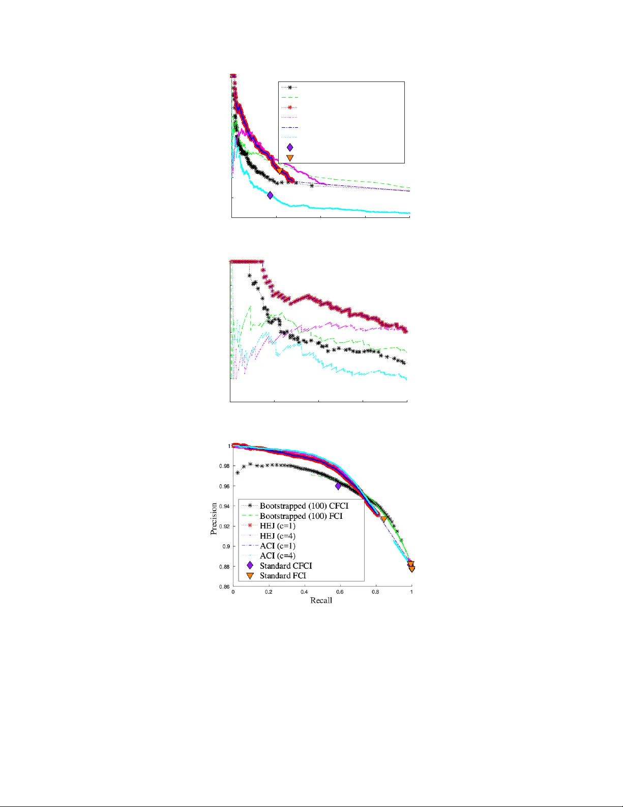
Authors: Sara Magliacane, Tom Claassen, Joris M. Mooij
Ancestral Causal Infer ence Sara Magliacane VU Amsterdam & Univ ersity of Amsterdam sara.magliacane@gmail.com T om Claassen Radboud Univ ersity Nijmegen tomc@cs.ru.nl Joris M. Mooij Univ ersity of Amsterdam j.m.mooij@uva.nl Abstract Constraint-based causal discovery from limited data is a notoriously dif ficult chal- lenge due to the many borderline independence test decisions. Se veral approaches to improv e the reliability of the predictions by exploiting redundanc y in the inde- pendence information ha ve been proposed recently . Though promising, existing approaches can still be greatly improv ed in terms of accuracy and scalability . W e present a nov el method that reduces the combinatorial explosion of the search space by using a more coarse-grained representation of causal information, drastically reducing computation time. Additionally , we propose a method to score causal pre- dictions based on their confidence. Crucially , our implementation also allows one to easily combine observational and interv entional data and to incorporate various types of available background knowledge. W e prove soundness and asymptotic consistency of our method and demonstrate that it can outperform the state-of- the-art on synthetic data, achie ving a speedup of sev eral orders of magnitude. W e illustrate its practical feasibility by applying it to a challenging protein data set. 1 Introduction Discov ering causal relations from data is at the foundation of the scientific method. Traditionally , cause-effect relations ha ve been recovered from experimental data in which the v ariable of interest is perturbed, b ut seminal w ork lik e the do -calculus [ 18 ] and the PC/FCI algorithms [ 25 , 28 ] demonstrate that, under certain assumptions (e.g., the well-known Causal Mark ov and F aithfulness assumptions [ 25 ]), it is already possible to obtain substantial causal information by using only observational data. Recently , there ha ve been se veral proposals for combining observ ational and experimental data to discov er causal relations. These causal discovery methods are usually di vided into two cate gories: constraint-based and score-based methods. Score-based methods typically ev aluate models using a penalized likelihood score, while constraint-based methods use statistical independences to express constraints o ver possible causal models. The adv antages of constraint-based ov er score-based methods are the ability to handle latent confounders and selection bias naturally , and that there is no need for parametric modeling assumptions. Additionally , constraint-based methods expressed in logic [ 2 , 3 , 27 , 9 ] allow for an easy integration of background knowledge, which is not trivial even for simple cases in approaches that are not based on logic [1]. T wo major disadvantages of traditional constraint-based methods are: (i) vulnerability to errors in statistical independence test results, which are quite common in real-world applications, (ii) no ranking or estimation of the confidence in the causal predictions. Se veral approaches address the first issue and impro ve the reliability of constraint-based methods by exploiting redundanc y in the independence information [ 3 , 9 , 27 ]. The idea is to assign weights to the input statements that reflect 29th Conference on Neural Information Processing Systems (NIPS 2016), Barcelona, Spain. their reliability , and then use a reasoning scheme that takes these weights into account. Sev eral weighting schemes can be defined, from simple ways to attach weights to single independence statements [ 9 ], to more complicated schemes to obtain weights for combinations of independence statements [ 27 , 3 ]. Unfortunately , these approaches ha ve to sacrifice either accuracy by using a greedy method [ 3 , 27 ], or scalability by formulating a discrete optimization problem on a super-e xponentially large search space [ 9 ]. Additionally , the confidence estimation issue is addressed only in limited cases [19]. W e propose Ancestral Causal Inference (A CI), a logic-based method that provides comparable accuracy to the best state-of-the-art constraint-based methods (e.g., [ 9 ]) for causal systems with latent v ariables without feedback, but impro ves on their scalability by using a more coarse-grained representation of causal information. Instead of representing all possible direct causal relations, in A CI we represent and reason only with ancestral relations (“indirect” causal relations), de veloping specialised ancestral reasoning rules. This representation, though still super-exponentially large, drastically reduces computation time. Moreov er , it turns out to be very conv enient, because in real-world applications the distinction between direct causal relations and ancestral relations is not always clear or necessary . Given the estimated ancestral relations, the estimation can be refined to direct causal relations by constraining standard methods to a smaller search space, if necessary . Furthermore, we propose a method to score predictions according to their confidence. The confidence score can be thought of as an approximation to the marginal probability of an ancestral relation. Scoring predictions enables one to rank them according to their reliability , allowing for higher accuracy . This is very important for practical applications, as the low reliability of the predictions of constraint-based methods has been a major impediment to their wide-spread use. W e prove soundness and asymptotic consistency under mild conditions on the statistical tests for ACI and our scoring method. W e show that A CI outperforms standard methods, like bootstrapped FCI and CFCI, in terms of accuracy , and achieves a speedup of se veral orders of magnitude o ver [ 9 ] on a synthetic dataset. W e illustrate its practical feasibility by applying it to a challenging protein data set [ 23 ] that so far had only been addressed with score-based methods and observ e that it successfully recov ers from faithfulness violations. In this context, we showcase the flexibility of logic-based approaches by introducing weighted ancestral relation constraints that we obtain from a combination of observ ational and interventional data, and show that they substantially increase the reliability of the predictions. Finally , we provide an open-source version of our algorithms and the ev aluation framew ork, which can be easily extended, at http://github.com/caus- am/aci . 2 Preliminaries and r elated work Preliminaries W e assume that the data generating process can be modeled by a causal Directed Acyclic Graph (D A G) that may contain latent v ariables. For simplicity we also assume that there is no selection bias. Finally , we assume that the Causal Marko v Assumption and the Causal F aithfulness Assumption [ 25 ] both hold. In other words, the conditional independences in the observational distribution correspond one-to-one with the d-separations in the causal D AG. Throughout the paper we represent variables with uppercase letters, while sets of variables are denoted by boldface. All proofs are provided in the Supplementary Material. A directed edge X → Y in the causal D AG represents a dir ect causal r elation between cause X on effect Y . Intuitiv ely , in this framework this indicates that manipulating X will produce a change in Y , while manipulating Y will hav e no effect on X . A more detailed discussion can be found in [ 25 ]. A sequence of directed edges X 1 → X 2 → · · · → X n is a dir ected path . If there exists a directed path from X to Y (or X = Y ), then X is an ancestor of Y (denoted as X 99K Y ). Otherwise, X is not an ancestor of Y (denoted as X 6 99K Y ). For a set of v ariables W , we write: X 99K W := ∃ Y ∈ W : X 99K Y , X 6 99K W := ∀ Y ∈ W : X 6 99K Y . (1) W e define an ancestral structur e as any non-strict partial order on the observed variables of the D AG, i.e., any relation that satisfies the follo wing axioms: ( r efle xivity ) : X 99K X, (2) ( transitivity ) : X 99K Y ∧ Y 99K Z = ⇒ X 99K Z, (3) ( antisymmetry ) : X 99K Y ∧ Y 99K X = ⇒ X = Y . (4) 2 The underlying causal D A G induces a unique “true” ancestral structure, which represents the transitive closure of the direct causal relations projected on the observed v ariables. For disjoint sets X , Y , W we denote conditional independence of X and Y giv en W as X ⊥ ⊥ Y | W , and conditional dependence as X 6 ⊥ ⊥ Y | W . W e call the cardinality | W | the or der of the conditional (in)dependence relation. Follo wing [ 2 ] we define a minimal conditional independence by: X ⊥ ⊥ Y | W ∪ [ Z ] := ( X ⊥ ⊥ Y | W ∪ Z ) ∧ ( X 6 ⊥ ⊥ Y | W ) , and similarly , a minimal conditional dependence by: X 6 ⊥ ⊥ Y | W ∪ [ Z ] := ( X 6 ⊥ ⊥ Y | W ∪ Z ) ∧ ( X ⊥ ⊥ Y | W ) . The square brack ets indicate that Z is needed for the (in)dependence to hold in the context of W . Note that the neg ation of a minimal conditional independence is not a minimal conditional dependence. Minimal conditional (in)dependences are closely related to ancestral relations, as pointed out in [2]: Lemma 1. F or disjoint (sets of) variables X , Y , Z, W : X ⊥ ⊥ Y | W ∪ [ Z ] = ⇒ Z 99K ( { X , Y } ∪ W ) , (5) X 6 ⊥ ⊥ Y | W ∪ [ Z ] = ⇒ Z 6 99K ( { X , Y } ∪ W ) . (6) Exploiting these rules (as well as others that will be introduced in Section 3) to deduce ancestral relations directly from (in)dependences is key to the greatly impro ved scalability of our method. Related work on conflict r esolution One of the earliest algorithms to deal with conflicting inputs in constraint-based causal discovery is Conserv ative PC [ 20 ], which adds “redundant” checks to the PC algorithm that allo w it to detect inconsistencies in the inputs, and then makes only predictions that do not rely on the ambiguous inputs. The same idea can be applied to FCI, yielding Conserv ativ e FCI (CFCI) [ 4 , 11 ]. BCCD (Bayesian Constraint-based Causal Discovery) [ 3 ] uses Bayesian confidence estimates to process information in decreasing order of reliability , discarding contradictory inputs as they arise. COmbINE (Causal discovery from Ov erlapping INtErventions) [ 27 ] is an algorithm that combines the output of FCI on sev eral overlapping observ ational and experimental datasets into a single causal model by first pooling and recalibrating the independence test p -values , and then adding each constraint incrementally in order of reliability to a SA T instance. Any constraint that makes the problem unsatisfiable is discarded. Our approach is inspired by a method presented by Hyttinen, Eberhardt and Järvisalo [ 9 ] (that we will refer to as HEJ in this paper), in which causal discovery is formulated as a constrained discrete minimization problem. Given a list of weighted independence statements, HEJ searches for the optimal causal graph G (an acyclic directed mixed graph, or ADMG) that minimizes the sum of the weights of the independence statements that are violated according to G . In order to test whether a causal graph G induces a certain independence, the method creates an encoding D AG of d-connection graphs . D-connection graphs are graphs that can be obtained from a causal graph through a series of operations (conditioning, marginalization and interv entions). An encoding D A G of d-connection graphs is a complex structure encoding all possible d-connection graphs and the sequence of operations that generated them from a giv en causal graph. This approach has been sho wn to correct errors in the inputs, but is computationally demanding because of the huge search space. 3 A CI: Ancestral Causal Inference W e propose Ancestral Causal Inference (A CI), a causal discovery method that accurately reconstructs ancestral structures, also in the presence of latent variables and statistical errors. A CI builds on HEJ [ 9 ], but rather than optimizing o ver encoding D AGs, A CI optimizes ov er the much simpler (but still very e xpressiv e) ancestral structures. For n variables, the number of possible ancestral structures is the number of partial orders ( http: //oeis.org/A001035 ), which grows as 2 n 2 / 4+ o ( n 2 ) [ 12 ], while the number of D AGs can be computed with a well-known super -exponential recurrence formula ( http://oeis.org/A003024 ). The number of ADMGs is | D AG( n ) | × 2 n ( n − 1) / 2 . Although still super-exponential, the number of ancestral structures grows asymptotically much slo wer than the number of DA Gs and ev en more so, ADMGs. For example, for 7 v ariables, there are 6 × 10 6 ancestral structures but already 2 . 3 × 10 15 ADMGs, which lower bound the number of encoding D A Gs of d-connection graphs used by HEJ. 3 New rules The rules in HEJ explicitly encode marginalization and conditioning operations on d-connection graphs, so they cannot be easily adapted to w ork directly with ancestral relations. Instead, A CI encodes the ancestral reasoning rules (2)–(6) and five no vel causal reasoning rules: Lemma 2. F or disjoint (sets) of variables X , Y , U, Z, W : ( X ⊥ ⊥ Y | Z ) ∧ ( X 6 99K Z ) = ⇒ X 6 99K Y , (7) X 6 ⊥ ⊥ Y | W ∪ [ Z ] = ⇒ X 6 ⊥ ⊥ Z | W , (8) X ⊥ ⊥ Y | W ∪ [ Z ] = ⇒ X 6 ⊥ ⊥ Z | W , (9) ( X ⊥ ⊥ Y | W ∪ [ Z ]) ∧ ( X ⊥ ⊥ Z | W ∪ U ) = ⇒ ( X ⊥ ⊥ Y | W ∪ U ) , (10) ( Z 6 ⊥ ⊥ X | W ) ∧ ( Z 6 ⊥ ⊥ Y | W ) ∧ ( X ⊥ ⊥ Y | W ) = ⇒ X 6 ⊥ ⊥ Y | W ∪ Z. (11) W e prove the soundness of the rules in the Supplementary Material. W e elaborate some conjectures about their completeness in the discussion after Theorem 1 in the next Section. Optimization of loss function W e formulate causal discovery as an optimization problem where a loss function is optimized over possible causal structures. Intuitiv ely , the loss function sums the weights of all the inputs that are violated in a candidate causal structure. Giv en a list I of weighted input statements ( i j , w j ) , where i j is the input statement and w j is the associated weight, we define the loss function as the sum of the weights of the input statements that are not satisfied in a gi ven possible structure W ∈ W , where W denotes the set of all possible causal structures. Causal discovery is formulated as a discrete optimization problem: W ∗ = arg min W ∈W L ( W ; I ) , (12) L ( W ; I ) := X ( i j ,w j ) ∈ I : W ∪R| = ¬ i j w j , (13) where W ∪ R | = ¬ i j means that input i j is not satisfied in structure W according to the rules R . This general formulation includes both HEJ and A CI, which differ in the types of possible structures W and the rules R . In HEJ W represents all possible causal graphs (specifically , acyclic directed mixed graphs, or ADMGs, in the acyclic case) and R are operations on d-connection graphs. In ACI W represent ancestral structures (defined with the rules(2)-(4)) and the rules R are rules (5)–(11). Constrained optimization in ASP The constrained optimization problem in (12) can be imple- mented using a variety of methods. Giv en the complexity of the rules, a formulation in an expressiv e logical language that supports optimization, e.g., Answer Set Programming (ASP), is very con venient. ASP is a widely used declarative programming language based on the stable model semantics [ 13 , 8 ] that has successfully been applied to se veral NP-hard problems. For A CI we use the state-of-the-art ASP solver clingo 4 [7]. W e provide the encoding in the Supplementary Material. W eighting schemes A CI supports two types of input statements: conditional independences and ancestral relations. These statements can each be assigned a weight that reflects their confidence. W e propose tw o simple approaches with the desirable properties of making A CI asymptotically consistent under mild assumptions (as described in the end of this Section), and assigning a much smaller weight to independences than to dependences (which agrees with the intuition that one is confident about a measured strong dependence, b ut not about independence vs. weak dependence). The approaches are: • a fr equentist approach, in which for any appropriate frequentist statistical test with indepen- dence as null hypothesis (resp. a non-ancestral relation), we define the weight: w = | log p − log α | , where p = p -v alue of the test , α = significance level (e.g., 5%) ; (14) • a Bayesian approach, in which the weight of each input statement i using data set D is: w = log p ( i |D ) p ( ¬ i |D ) = log p ( D | i ) p ( D |¬ i ) p ( i ) p ( ¬ i ) , (15) where the prior probability p ( i ) can be used as a tuning parameter . 4 Giv en observ ational and interventional data, in which each intervention has a single known tar get (in particular , it is not a fat-hand intervention [ 5 ]), a simple way to obtain a weighted ancestral statement X 99K Y is with a two-sample test that tests whether the distrib ution of Y changes with respect to its observational distribution when interv ening on X . This approach con veniently applies to v arious types of interventions: perfect interventions [ 18 ], soft interventions [ 15 ], mechanism changes [ 26 ], and activity interv entions [ 17 ]. The two-sample test can also be implemented as an independence test that tests for the independence of Y and I X , the indicator variable that has v alue 0 for observational samples and 1 for samples from the interventional distribution in which X has been intervened upon. 4 Scoring causal predictions The constrained minimization in (12) may produce several optimal solutions, because the underlying structure may not be identifiable from the inputs. T o address this issue, we propose to use the loss function (13) and score the confidence of a feature f (e.g., an ancestral relation X 99K Y ) as: C ( f ) = min W ∈W L ( W ; I ∪ { ( ¬ f , ∞ ) } ) − min W ∈W L ( W ; I ∪ { ( f , ∞ ) } ) . (16) W ithout going into details here, we note that the confidence (16) can be interpreted as a MAP approximation of the log-odds ratio of the probability that feature f is true in a Markov Logic model: P ( f | I , R ) P ( ¬ f | I , R ) = P W ∈W e −L ( W ; I ) 1 W ∪R| = f P W ∈W e −L ( W ; I ) 1 W ∪R| = ¬ f ≈ max W ∈W e −L ( W ; I ∪{ ( f , ∞ ) } ) max W ∈W e −L ( W ; I ∪{ ( ¬ f , ∞ ) } ) = e C ( f ) . In this paper, we usually consider the features f to be ancestral relations, but the idea is more generally applicable. For example, combined with HEJ it can be used to score direct causal relations. Soundness and completeness Our scoring method is sound for oracle inputs: Theorem 1. Let R be sound (not necessarily complete) causal r easoning rules. F or any featur e f , the confidence scor e C ( f ) of (16) is sound for oracle inputs with infinite weights. Here, soundness means that C ( f ) = ∞ if f is identifiable from the inputs, C ( f ) = −∞ if ¬ f is identifiable from the inputs, and C ( f ) = 0 otherwise (neither are identifiable). As features, we can consider for example ancestral relations f = X 99K Y for v ariables X, Y . W e conjecture that the rules (2)–(11) are “order-1-complete”, i.e., the y allow one to deduce all (non)ancestral relations that are identifiable from oracle conditional independences of order ≤ 1 in observ ational data. For higher-order inputs additional rules can be deriv ed. Ho wev er , our primary interest in this work is improving computation time and accuracy , and we are willing to sacrifice completeness. A more detailed study of the completeness properties is left as future work. Asymptotic consistency Denote the number of samples by N . For the frequentist weights in (14), we assume that the statistical tests are consistent in the following sense: log p N − log α N P → −∞ H 1 + ∞ H 0 , (17) as N → ∞ , where the null hypothesis H 0 is independence/nonancestral relation and the alternati ve hypothesis H 1 is dependence/ancestral relation. Note that we need to choose a sample-size dependent threshold α N such that α N → 0 at a suitable rate. Kalisch and Bühlmann [ 10 ] show ho w this can be done for partial correlation tests under the assumption that the distribution is multi variate Gaussian. For the Bayesian weighting scheme in (15), we assume that for N → ∞ , w N P → −∞ if i is true + ∞ if i is false . (18) This will hold (as long as there is no model misspecification) under mild technical conditions for finite-dimensional exponential family models. In both cases, the probability of a type I or type II error will con verge to 0, and in addition, the corresponding weight will con verge to ∞ . Theorem 2. Let R be sound (not necessarily complete) causal r easoning rules. F or any featur e f , the confidence scor e C ( f ) of (16) is asymptotically consistent under assumption (17) or (18). Here, “asymptotically consistent” means that the confidence score C ( f ) → ∞ in probability if f is identifiably true, C ( f ) → −∞ in probability if f is identifiably false, and C ( f ) → 0 in probability otherwise. 5 A verage execution time (s) n c ACI HEJ B AFCI B ACFCI 6 1 0.21 12.09 8.39 12.51 6 4 1.66 432.67 11.10 16.36 7 1 1.03 715.74 9.37 15.12 8 1 9.74 ≥ 2500 13.71 21.71 9 1 146.66 2500 18.28 28.51 (a) 0.1$ 1$ 10$ 100$ 1000$ 10000$ 1$ 101$ 201$ 301$ 401$ 501$ 601$ 701$ 801$ 901$ 1001$ 1101$ 1201$ 1301$ 1401$ 1501$ 1601$ 1701$ 1801$ 1901$ Execution$time$(s)$ Instances$(sorted$by$solution$time)$ HEJ$ ACI$ (b) Figure 1: Execution time comparison on synthetic data for the frequentist test on 2000 synthetic models: (a) average ex ecution time for different combinations of number of variables n and max. order c ; (b) detailed plot of ex ecution times for n = 7 , c = 1 (logarithmic scale). 5 Evaluation In this section we report ev aluations on synthetically generated data and an application on a real dataset. Crucially , in causal discovery precision is often more important than recall. In many real- world applications, disco vering a few high-confidence causal relations is more useful than finding ev ery possible causal relation, as reflected in recently proposed algorithms, e.g., [19]. Compared methods W e compare the predictions of A CI and of the acyclic causally insuf ficient version of HEJ [ 9 ], when used in combination with our scoring method (16). W e also ev aluate two standard methods: Anytime FCI [ 24 , 28 ] and Anytime CFCI [ 4 ], as implemented in the pcalg R package [ 11 ]. W e use the anytime versions of (C)FCI because they allow for independence test results up to a certain order . W e obtain the ancestral relations from the output P AG using Theorem 3.1 from [ 22 ]. (Anytime) FCI and CFCI do not rank their predictions, but only predict the type of relation: ancestral (which we conv ert to +1), non-ancestral (-1) and unknown (0). T o get a scoring of the predictions, we also compare with bootstrapped versions of Anytime FCI and Anytime CFCI. W e perform the bootstrap by repeating the following procedure 100 times: sample randomly half of the data, perform the independence tests, run Anytime (C)FCI. From the 100 output P AGs we extract the ancestral predictions and a verage them. W e refer to these methods as B A(C)FCI. For a fair comparison, we use the same independence tests and thresholds for all methods. Synthetic data W e simulate the data using the simulator from HEJ [ 9 ]: for each experimental condition (e.g., a giv en number of variables n and order c ), we generate randomly M linear acyclic models with latent variables and Gaussian noise and sample N = 500 data points. W e then perform independence tests up to order c and weight the (in)dependence statements using the weighting schemes described in Section 3. For the frequentist weights we use tests based on partial correlations and Fisher’ s z -transform to obtain approximate p -values (see, e.g., [ 10 ]) with significance level α = 0 . 05 . For the Bayesian weights, we use the Bayesian test for conditional independence presented in [14] as implemented by HEJ with a prior probability of 0.1 for independence. In Figure 1(a) we show the av erage ex ecution times on a single core of a 2.80GHz CPU for different combinations of n and c , while in Figure 1(b) we show the ex ecution times for n = 7 , c = 1 , sorting the ex ecution times in ascending order . For 7 v ariables A CI is almost 3 orders of magnitude faster than HEJ, and the difference gro ws exponentially as n increases. For 8 v ariables HEJ can complete only four of the first 40 simulated models before the timeout of 2500 s. F or reference we add the ex ecution time for bootstrapped anytime FCI and CFCI. In Figure 2 we sho w the accurac y of the predictions with precision-recall (PR) curv es for both ancestral ( X 99K Y ) and nonancestral ( X 6 99K Y ) relations, in dif ferent settings. In this Figure, for A CI and HEJ all of the results are computed using frequentist weights and, as in all ev aluations, our scoring method (16). While for these two methods we use c = 1 , for (bootstrapped) (C)FCI we use all possible independence test results ( c = n − 2 ). In this case, the an ytime versions of FCI and CFCI are equiv alent to the standard versions of FCI and CFCI. Since the overall results are similar , we report the results with the Bayesian weights in the Supplementary Material. In the first row of Figure 2, we show the setting with n = 6 variables. The performances of HEJ and A CI coincide, performing significantly better for nonancestral predictions and the top ancestral 6 Recall 0 0.05 0.1 0.15 0.2 Precision 0.3 0.4 0.5 0.6 0.7 0.8 0.9 1 Bootstrapped (100) CFCI Bootstrapped (100) FCI HEJ (c=1) ACI (c=1) Standard CFCI Standard FCI (a) PR ancestral: n=6 Recall 0 0.005 0.01 0.015 0.02 Precision 0.6 0.65 0.7 0.75 0.8 0.85 0.9 0.95 1 (b) PR ancestral: n=6 (zoom) (c) PR nonancestral: n=6 Recall 0 0.05 0.1 0.15 0.2 Precision 0.3 0.4 0.5 0.6 0.7 0.8 0.9 1 Bootstrapped (100) CFCI Bootstrapped (100) FCI ACI (c=1) ACI (c=1, i=1) Standard CFCI Standard FCI (d) PR ancestral: n=8 Recall 0 0.005 0.01 0.015 0.02 Precision 0.3 0.4 0.5 0.6 0.7 0.8 0.9 1 (e) PR ancestral: n=8 (zoom) (f) PR nonancestral: n=8 Figure 2: Accuracy on synthetic data for the tw o prediction tasks (ancestral and nonancestral relations) using the frequentist test with α = 0 . 05 . The left column sho ws the precision-recall curve for ancestral predictions, the middle column sho ws a zoomed-in version in the interv al (0,0.02), while the right column shows the nonancestral predictions. predictions (see zoomed-in version in Figure 2(b)). This is remarkable, as HEJ and A CI use only independence test results up to order c = 1 , in contrast with (C)FCI which uses independence test results of all orders. Interestingly , the two discrete optimization algorithms do not seem to benefit much from higher order independence tests, thus we omit them from the plots (although we add the graphs in the Supplementary Material). Instead, bootstrapping traditional methods, oblivious to the (in)dependence weights, seems to produce surprisingly good results. Nevertheless, both A CI and HEJ outperform bootstrapped FCI and CFCI, suggesting these methods achie ve nontri vial error-correction. In the second ro w of Figure 2, we sho w the setting with 8 v ariables. In this setting HEJ is too slow . In addition to the previous plot, we plot the accurac y of ACI when there is oracle background kno wledge on the descendants of one v ariable ( i = 1 ). This setting simulates the ef fect of using interventional data, and we can see that the performance of A CI improves significantly , especially in the ancestral preditions. The performance of (bootstrapped) FCI and CFCI is limited by the fact that the y cannot take adv antage of this background kno wledge, except with complicated postprocessing [1]. Application on r eal data W e consider the challenging task of reconstructing a signalling network from flo w cytometry data [ 23 ] under different experimental conditions. Here we consider one experimental condition as the observ ational setting and se ven others as interv entional settings. More details and more e v aluations are reported in the Supplementary Material. In contrast to likelihood- based approaches like [ 23 , 5 , 17 , 21 ], in our approach we do not need to model the interventions quantitativ ely . W e only need to know the intervention tar gets , while the intervention types do not matter . Another advantage of our approach is that it takes into account possible latent v ariables. W e use a t -test to test for each intervention and for each variable whether its distribution changes with respect to the observ ational condition. W e use the p -values of these tests as in (14) in order to obtain weighted ancestral relations that are used as input (with threshold α = 0 . 05 ). For example, if adding U0126 (a MEK inhibitor) changes the distrib ution of RAF significantly with respect to the observ ational baseline, we get a weighted ancestral relation MEK 99K RAF . In addition, we use partial correlations up to order 1 (tested in the observational data only) to obtain weighted independences used as input. W e use A CI with (16) to score the ancestral relations for each ordered pair of variables. The main results are illustrated in Figure 3, where we compare A CI with bootstrapped anytime CFCI 7 Raf Mek PLCg PIP2 PIP3 Erk Akt PKA PKC p38 JNK BCFCI (indep. <= 1) Raf Mek PLCg PIP2 PIP3 Erk Akt PKA PKC p38 JNK (a) Bootstrapped (100) any- time CFCI (input: indepen- dences of order ≤ 1 ) Raf Mek PLCg PIP2 PIP3 Erk Akt PKA PKC p38 JNK ACI (ancestral relations) Raf Mek PLCg PIP2 PIP3 Erk Akt PKA PKC p38 JNK (b) A CI (input: weighted an- cestral relations) Raf Mek PLCg PIP2 PIP3 Erk Akt PKA PKC p38 JNK ACI (ancestral r. + indep. <= 1) Raf Mek PLCg PIP2 PIP3 Erk Akt PKA PKC p38 JNK (c) ACI (input: independences of order ≤ 1 , weighted ances- tral relations) Weighted causes(i,j) Raf Mek PLCg PIP2 PIP3 Erk Akt PKA PKC p38 JNK Raf Mek PLCg PIP2 PIP3 Erk Akt PKA PKC p38 JNK − 1000 − 500 0 500 1000 Weighted indep(i,j) Raf Mek PLCg PIP2 PIP3 Erk Akt PKA PKC p38 JNK Raf Mek PLCg PIP2 PIP3 Erk Akt PKA PKC p38 JNK − 1000 − 500 0 500 1000 Consensus graph Raf Mek PLCg PIP2 PIP3 Erk Akt PKA PKC p38 JNK Raf Mek PLCg PIP2 PIP3 Erk Akt PKA PKC p38 JNK − 1000 − 500 0 500 1000 ACI (causes) Raf Mek PLCg PIP2 PIP3 Erk Akt PKA PKC p38 JNK Raf Mek PLCg PIP2 PIP3 Erk Akt PKA PKC p38 JNK − 1000 − 500 0 500 1000 ACI (causes + indeps) Raf Mek PLCg PIP2 PIP3 Erk Akt PKA PKC p38 JNK Raf Mek PLCg PIP2 PIP3 Erk Akt PKA PKC p38 JNK − 1000 − 500 0 500 1000 FCI Raf Mek PLCg PIP2 PIP3 Erk Akt PKA PKC p38 JNK Raf Mek PLCg PIP2 PIP3 Erk Akt PKA PKC p38 JNK − 1000 − 500 0 500 1000 CFCI Raf Mek PLCg PIP2 PIP3 Erk Akt PKA PKC p38 JNK Raf Mek PLCg PIP2 PIP3 Erk Akt PKA PKC p38 JNK − 1000 − 500 0 500 1000 Acyclic Joris graph Raf Mek PLCg PIP2 PIP3 Erk Akt PKA PKC p38 JNK Raf Mek PLCg PIP2 PIP3 Erk Akt PKA PKC p38 JNK − 1000 − 500 0 500 1000 Figure 3: Results for flo w cytometry dataset. Each matrix represents the ancestral relations, where each row represents a cause and each column an effect. The colors encode the confidence lev els: green is positi ve, black is unkno wn, while red is ne gati ve. The intensity of the color represents the degree of confidence. For e xample, A CI identifies MEK to be a cause of RAF with high confidence. under different inputs. The output for boostrapped anytime FCI is similar , so we report it only in the Supplementary Material. Algorithms like (anytime) (C)FCI can only use the independences in the observational data as input and therefore miss the strongest signal, weighted ancestral r elations , which are obtained by comparing interventional with observational data. In the Supplementary Material, we compare also with other methods ([ 19 ], [ 17 ]). Interestingly , as we show there, our results are similar to the best acyclic model reconstructed by the score-based method from [ 17 ]. As for other constraint-based methods, HEJ is computationally unfeasible in this setting, while COMBINE assumes perfect interventions (while this dataset contains mostly acti vity interventions). Notably , our algorithms can correctly recov er from faithfulness violations (e.g., the independence between MEK and ERK), because they take into account the weight of the input statements (the weight of the independence is considerably smaller than that of the ancestral relation, which corresponds with a quite significant change in distrib ution). In contrast, methods that start by reconstructing the skeleton, like (an ytime) (C)FCI, would decide that MEK and ERK are nonadjacent, and are unable to recov er from that erroneous decision. This illustrates another advantage of our approach. 6 Discussion and conclusions As we have shown, ancestral structures are very well-suited for causal discovery . They offer a natural way to incorporate background causal kno wledge, e.g., from experimental data, and allo w a huge computational advantage o ver e xisting representations for error-correcting algorithms, such as [ 9 ]. When needed, ancestral structures can be mapped to a finer -grained representation with direct causal relations, as we sketch in the Supplementary Material. Furthermore, confidence estimates on causal predictions are extremely helpful in practice, and can significantly boost the reliability of the output. Although standard methods, like bootstrapping (C)FCI, already provide reasonable estimates, methods that take into account the confidence in the inputs, as the one presented here, can lead to further improv ements of the reliability of causal relations inferred from data. Strangely (or fortunately) enough, neither of the optimization methods seems to improve much with higher order independence test results. W e conjecture that this may happen because our loss function essentially assumes that the test results are independent from another (which is not true). Finding a way to tak e this into account in the loss function may further impro ve the achie vable accurac y , but such an extension may not be straightforward. Acknowledgments SM and JMM were supported by NW O, the Netherlands Org anization for Scientific Research (VIDI grant 639.072.410). SM was also supported by the Dutch programme COMMIT/ under the Data2Semantics project. TC was supported by NWO grant 612.001.202 (MoCoCaDi), and EU-FP7 grant agreement n.603016 (MA TRICS). W e also thank Sofia T riantafillou for her feedback, especially for pointing out the correct way to read ancestral relations from a P AG. 8 7 Proofs 7.1 A CI causal reasoning rules W e giv e a combined proof of all the ACI reasoning rules. Note that the numbering of the rules here is different from the numbering used in the main paper . Lemma 3. F or X , Y , Z , U , W disjoint (sets of) variables: 1. ( X ⊥ ⊥ Y | W ) ∧ ( X 6 99K W ) = ⇒ X 6 99K Y 2. X 6 ⊥ ⊥ Y | W ∪ [ Z ] = ⇒ ( X 6 ⊥ ⊥ Z | W ) ∧ ( Z 6 99K { X, Y } ∪ W ) 3. X ⊥ ⊥ Y | W ∪ [ Z ] = ⇒ ( X 6 ⊥ ⊥ Z | W ) ∧ ( Z 99K { X , Y } ∪ W ) 4. ( X ⊥ ⊥ Y | W ∪ [ Z ]) ∧ ( X ⊥ ⊥ Z | W ∪ U ) = ⇒ ( X ⊥ ⊥ Y | W ∪ U ) 5. ( Z 6 ⊥ ⊥ X | W ) ∧ ( Z 6 ⊥ ⊥ Y | W ) ∧ ( X ⊥ ⊥ Y | W ) = ⇒ X 6 ⊥ ⊥ Y | W ∪ Z Pr oof. W e assume a causal D A G with possible latent variables, the causal Marko v assumption, and the causal faithfulness assumption. 1. This is a strengthened version of rule R 2 (i) in [ 6 ]: note that the additional assumptions made there ( Y 6 99K W , Y 6 99K X ) are redundant and not actually used in their proof. For completeness, we gi ve the proof here. If X 99K Y , then there is a directed path from X to Y . As all paths between X and Y are blocked by W , the directed path from X to Y must contain a node W ∈ W . Hence X 99K W , a contradiction with X 6 99K W . 2. If X 6 ⊥ ⊥ Y | W ∪ [ Z ] then there exists a path π between X and Y such that each noncollider on π is not in W ∪ { Z } , ev ery collider on π is ancestor of W ∪ { Z } , and there exists a collider on π that is ancestor of Z but not of W . Let C be the collider on π closest to X that is ancestor of Z but not of W . Note that (a) The path X · · · C → · · · → Z is d-connected gi ven W . (b) Z 6 99K W (because otherwise C 99K Z 99K W , a contradiction). (c) Z 6 99K Y (because otherwise the path X · · · C → · · · → Z → · · · → Y would be d-connected giv en W , a contradiction). Hence we conclude that X 6 ⊥ ⊥ Z | W , Z 6 99K W , Z 6 99K Y , and by symmetry also Z 6 99K X . 3. Suppose X ⊥ ⊥ Y | W ∪ [ Z ] . Then there exists a path π between X and Y , such that each noncollider on π is not in W , each collider on π is an ancestor of W , and Z is a noncollider on π . Note that (a) The subpath X · · · Z must be d-connected given W . (b) Z has at least one outgoing edge on π . Follo w this edge further along π until reaching either X , Y , or the first collider . When a collider is reached, follo w the directed path to W . Hence there is a directed path from Z to X or Y or to W , i.e., Z 99K { X , Y } ∪ W . 4. If in addition, X ⊥ ⊥ Z | W ∪ U , then U must be a noncollider on the subpath X · · · Z . Therefore, X ⊥ ⊥ Y | W ∪ U . 5. Assume that Z 6 ⊥ ⊥ X | W and Z 6 ⊥ ⊥ Y | W . Then there must be paths π between Z and X and ρ between Z and Y such that each noncollider is not in W and each collider is ancestor of W . Let U be the node on π closest to X that is also on ρ (this could be Z ). Then we hav e a path X · · · U · · · Y such that each collider (except U ) is ancestor of W and each noncollider (except U ) is not in W . This path must be blocked gi ven W as X ⊥ ⊥ Y | W . If U would be a noncollider on this path, it would need to be in W in order to block it; howe ver , it must then also be a noncollider on π or ρ and hence cannot be in W . Therefore, U must be a collider on this path and cannot be ancestor of W . W e have to sho w that U is ancestor of Z . If U were a collider on π or ρ , it would be ancestor of W , a contradiction. Hence U must hav e an outgoing arro w pointing to wards Z on π and ρ . If we encounter a collider following the directed edges, we get a contradiction, as that collider , and hence U , would be ancestor of W . Hence U is ancestor of Z , and therefore, X 6 ⊥ ⊥ Y | W ∪ Z . 9 7.2 Soundness Theorem 3. Let R be sound (not necessarily complete) causal r easoning rules. F or any featur e f , the confidence scor e C ( f ) of (16) is sound for oracle inputs with infinite weights, i.e., C ( f ) = ∞ if f is identifiable fr om the inputs, C ( f ) = −∞ if ¬ f is identifiable fr om the inputs, and C ( f ) = 0 otherwise (neither ar e identifiable). Pr oof. W e assume that the data generating process is described by a causal D A G which may contain additional latent variables, and that the distrib utions are faithful to the D AG. The theorem then follo ws directly from the soundness of the rules and the soundness of logical reasoning. 7.3 Asymptotic consistency of scoring method Theorem 4. Let R be sound (not necessarily complete) causal r easoning rules. F or any featur e f , the confidence scor e C ( f ) of (16) is asymptotically consistent under assumption (14) or (15) in the main paper , i.e., • C ( f ) → ∞ in probability if f is identifiably true, • C ( f ) → −∞ in probability if f is identifiably false, • C ( f ) → 0 in probability otherwise (neither ar e identifiable). Pr oof. As the number of statistical tests is fixed (or at least bounded from abo ve), the probability of any error in the test results con verges to 0 asymptotically . The loss function of all structures that do not correspond with the properties of the true causal D AG con ver ges to + ∞ in probability , whereas the loss function of all structures that are compatible with properties of the true causal D AG con ver ges to 0 in probability . 8 Additional results on synthetic data In Figures 4 and 5 we sho w the performance of A CI and HEJ [ 9 ] for higher order independence test results ( c = 4 ). As in the main paper , for (bootstrapped) FCI and CFCI we use c = 4 , because it gives the best predictions for these methods. In Figure 4 we report more accuracy results on the frequentist test with α = 0 . 05 , the same setting as Figure 2 (a-c) in the main paper . As we see, the performances of A CI and HEJ do not really improve with higher order b ut actually seem to deteriorate. In Figure 5 we report accuracy results on synthetic data also for the Bayesian test described in the main paper, with prior probability of independence p = 0 . 1 . Using the Bayesian test does not change the ov erall conclusions: ACI and HEJ o verlap for order c = 1 and they perform better than bootstrapped (C)FCI. 10 Recall 0 0.02 0.04 0.06 0.08 0.1 0.12 0.14 0.16 0.18 0.2 Precision 0 0.1 0.2 0.3 0.4 0.5 0.6 0.7 0.8 0.9 1 Bootstrapped (100) CFCI Bootstrapped (100) FCI HEJ (c=1) HEJ (c=4) ACI (c=1) ACI (c=4) Standard CFCI Standard FCI (a) PR ancestral Recall 0 0.002 0.004 0.006 0.008 0.01 0.012 0.014 0.016 0.018 0.02 Precision 0 0.1 0.2 0.3 0.4 0.5 0.6 0.7 0.8 0.9 1 (b) PR ancestral (zoom) (c) PR nonancestral Figure 4: Synthetic data: accuracy for the two prediction tasks (ancestral and nonancestral relations) for n = 6 variables using the frequentist test with α = 0 . 05 , also for higher order c . 9 A pplication on real data W e provide more details and more results on the real-world dataset that was briefly described in the main paper, the flo w cytometry data [ 23 ]. The data consists of simultaneous measurements of expression le vels of 11 biochemical agents in individual cells of the human immune system under 14 different e xperimental conditions. 11 Recall 0 0.05 0.1 0.15 0.2 Precision 0.3 0.4 0.5 0.6 0.7 0.8 0.9 1 Bootstrapped (100) CFCI Bootstrapped (100) FCI HEJ (c=1) HEJ (c=4) ACI (c=1) ACI (c=4) Standard CFCI Standard FCI (a) PR ancestral Recall 0 0.005 0.01 0.015 0.02 Precision 0.4 0.5 0.6 0.7 0.8 0.9 1 (b) PR ancestral (zoom) (c) PR nonancestral Figure 5: Synthetic data: accuracy for the two prediction tasks (ancestral and nonancestral relations) for n = 6 variables using the Bayesian test with prior probability of independence p = 0 . 1 . 9.1 Experimental conditions The experimental conditions can be grouped into two batches of 8 conditions each that hav e very similar interventions: • “no-ICAM”, used in the main paper and commonly used in the literature; 12 T able 1: Reagents used in the various experimental conditions in [ 23 ] and corresponding intervention types and targets. The intervention types and tar gets are based on (our interpretation of) biological background kno wledge. The upper table describes the “no-ICAM” batch of conditions that is most commonly used in the literature. The lo wer table describes the additional “ICAM” batch of conditions that we also use here. no-ICAM: Reagents Intervention α -CD3, α -CD28 ICAM-2 Additional T arget T ype + - - - (observational) + - AKT inhibitor AKT activity + - G0076 PKC activity + - Psitectorigenin PIP2 abundance + - U0126 MEK activity + - L Y294002 PIP2/PIP3 mechanism change - - PMA PKC acti vity + fat-hand - - β 2CAMP PKA activity + f at-hand ICAM: Reagents Intervention α -CD3, α -CD28 ICAM-2 Additional T arget T ype + + - - (observational) + + AKT inhibitor AKT activity + + G0076 PKC activity + + Psitectorigenin PIP2 abundance + + U0126 MEK activity + + L Y294002 PIP2/PIP3 mechanism change - - PMA PKC acti vity + fat-hand - - β 2CAMP PKA activity + f at-hand • “ICAM”, where Intercellular Adhesion Protein-2 (ICAM-2) was added (except when PMA or β 2CAMP was added). For each batch of 8 conditions, the e xperimenters added α -CD3 and α -CD28 to activ ate the signaling network in 6 out of 8 conditions. For the remaining tw o conditions (PMA and β 2CAMP), α -CD3 and α -CD28 were not added (and neither was ICAM-2). W e can consider the absence of these stimuli as a global intervention relati ve to the observational baseline (where α -CD3 and α -CD28 are present, and in addition ICAM-2 is present in the ICAM batch). For each batch (ICAM and no-ICAM), we can consider an observational dataset and 7 interventional datasets with dif ferent activ ators and inhibitors added to the cells, as described in T able 1. Note that the datasets from the last two conditions are the same in both settings. For more information about intervention types, see [17]. In this paper , we ignore the fact that in the last tw o interventional datasets in each batch (PMA and β 2CAMP) there is also a global intervention. Ignoring the global intervention allo ws us to compute the weighted ancestral relations, since we consider any variable that changes its distribution with respect to the observ ational condition to be an effect of the main tar get of the intervention (PKC for PMA and PKA for β 2CAMP). This is in line with pre vious work [ 23 , 17 ]. Also, we consider only PIP3 as the main target of the L Y294002 intervention, based on the consensus network [ 23 ], ev en though in [ 17 ] both PIP2 and PIP3 are considered to be targets of this intervention. In future work, we plan to extend A CI in order to address the task of learning the intervention tar gets from data, as done by [5] for a score-based approach. In the main paper we provide some results for the most commonly used no-ICAM batch of e xperimen- tal conditions. Below we report additional results on the same batch. Moreover , we provide results for causal discov ery on the ICAM batch, which are quite consistent with the no-ICAM batch. Finally , we compare with other methods that were applied to this dataset, especially with a score-based approach ([17]) that shows surprisingly similar results to A CI, although it uses a very dif ferent method. 13 Raf Mek PLCg PIP2 PIP3 Erk Akt PKA PKC p38 JNK Independences (order 0) Raf Mek PLCg PIP2 PIP3 Erk Akt PKA PKC p38 JNK (a) Independences of order 0 Raf Mek PLCg PIP2 PIP3 Erk Akt PKA PKC p38 JNK Ancestral relations Raf Mek PLCg PIP2 PIP3 Erk Akt PKA PKC p38 JNK (b) W eighted ancestral relations Weighted causes(i,j) Raf Mek PLCg PIP2 PIP3 Erk Akt PKA PKC p38 JNK Raf Mek PLCg PIP2 PIP3 Erk Akt PKA PKC p38 JNK − 1000 − 500 0 500 1000 Weighted indep(i,j) Raf Mek PLCg PIP2 PIP3 Erk Akt PKA PKC p38 JNK Raf Mek PLCg PIP2 PIP3 Erk Akt PKA PKC p38 JNK − 1000 − 500 0 500 1000 Consensus graph Raf Mek PLCg PIP2 PIP3 Erk Akt PKA PKC p38 JNK Raf Mek PLCg PIP2 PIP3 Erk Akt PKA PKC p38 JNK − 1000 − 500 0 500 1000 ACI (causes) Raf Mek PLCg PIP2 PIP3 Erk Akt PKA PKC p38 JNK Raf Mek PLCg PIP2 PIP3 Erk Akt PKA PKC p38 JNK − 1000 − 500 0 500 1000 ACI (causes + indeps) Raf Mek PLCg PIP2 PIP3 Erk Akt PKA PKC p38 JNK Raf Mek PLCg PIP2 PIP3 Erk Akt PKA PKC p38 JNK − 1000 − 500 0 500 1000 FCI Raf Mek PLCg PIP2 PIP3 Erk Akt PKA PKC p38 JNK Raf Mek PLCg PIP2 PIP3 Erk Akt PKA PKC p38 JNK − 1000 − 500 0 500 1000 CFCI Raf Mek PLCg PIP2 PIP3 Erk Akt PKA PKC p38 JNK Raf Mek PLCg PIP2 PIP3 Erk Akt PKA PKC p38 JNK − 1000 − 500 0 500 1000 Acyclic Joris graph Raf Mek PLCg PIP2 PIP3 Erk Akt PKA PKC p38 JNK Raf Mek PLCg PIP2 PIP3 Erk Akt PKA PKC p38 JNK − 1000 − 500 0 500 1000 Raf Mek PLCg PIP2 PIP3 Erk Akt PKA PKC p38 JNK ACI (independences <= 1) Raf Mek PLCg PIP2 PIP3 Erk Akt PKA PKC p38 JNK (d) A CI (input: independences or- der ≤ 1 ) Raf Mek PLCg PIP2 PIP3 Erk Akt PKA PKC p38 JNK ACI (ancestral relations) Raf Mek PLCg PIP2 PIP3 Erk Akt PKA PKC p38 JNK (e) A CI (input: weighted ances- tral relations) Raf Mek PLCg PIP2 PIP3 Erk Akt PKA PKC p38 JNK ACI (ancestral r. + indep. <= 1) Raf Mek PLCg PIP2 PIP3 Erk Akt PKA PKC p38 JNK (f) ACI (input: independences or- der ≤ 1 , weighted ancestral rela- tions) Raf Mek PLCg PIP2 PIP3 Erk Akt PKA PKC p38 JNK BFCI (indep. <= 1) Raf Mek PLCg PIP2 PIP3 Erk Akt PKA PKC p38 JNK (g) Bootstrapped (100) anytime FCI (input: independences order ≤ 1 ) Raf Mek PLCg PIP2 PIP3 Erk Akt PKA PKC p38 JNK BCFCI (indep. <= 1) Raf Mek PLCg PIP2 PIP3 Erk Akt PKA PKC p38 JNK (h) Bootstrapped (100) anytime CFCI (input: independences or- der ≤ 1 ) Figure 6: Results on flow c ytometry dataset, no-ICAM batch. The top row represents some of the possible inputs: weighted independences of order 0 from the observational dataset (the inputs include also order 1 test results, but these are not visualized here) and weighted ancestral relations recovered from comparing the interventional datasets with the observational data. In the bottom two rows each matrix represents the ancestral relations that are estimated using dif ferent inputs and different methods (A CI, bootstrapped anytime FCI or CFCI). Each ro w represents a cause, while the columns are the ef fects. The colors encodes the confidence lev els, green is positi ve, black is unkno wn, while red is negati ve. The intensity of the color represents the degree of confidence. 9.2 Results on no-ICAM batch In Figure 6 we pro vide additional results for the no-ICAM batch. In the first row we sho w some of the possible inputs: weighted independences (in this case partial correlations) from observ ational data and weighted ancestral relations from comparing the interventional datasets with the observ ational data. Specifically , we consider as inputs only independences up to order 1 (but only independences of order 0 are visualized in the figure). The color encodes the weight of the independence. As an example, the heatmap sho ws that Raf and Mek are strongly dependent. For the weighted ancestral relations, in Figure 6 we plot a matrix in which each row represents a cause, while the columns are the ef fects. As described in the main paper we use a t -test to test for each intervention and for each v ariable whether its distribution changes with respect to the observational condition. W e use the biological knowledge summarised in T able 1 to define the intervention tar get, which is then considered the putati ve “cause”. Then we use the p -v alues of these tests and a threshold α = 0 . 05 to obtain the weights of the ancestral relations, similarly to what is proposed in the main 14 Raf Mek PLCg PIP2 PIP3 Erk Akt PKA PKC p38 JNK Independences (order 0) Raf Mek PLCg PIP2 PIP3 Erk Akt PKA PKC p38 JNK (a) Independences of order 0 Raf Mek PLCg PIP2 PIP3 Erk Akt PKA PKC p38 JNK Ancestral relations Raf Mek PLCg PIP2 PIP3 Erk Akt PKA PKC p38 JNK (b) W eighted ancestral relations Weighted causes(i,j) Raf Mek PLCg PIP2 PIP3 Erk Akt PKA PKC p38 JNK Raf Mek PLCg PIP2 PIP3 Erk Akt PKA PKC p38 JNK − 1000 − 500 0 500 1000 Weighted indep(i,j) Raf Mek PLCg PIP2 PIP3 Erk Akt PKA PKC p38 JNK Raf Mek PLCg PIP2 PIP3 Erk Akt PKA PKC p38 JNK − 1000 − 500 0 500 1000 Consensus graph Raf Mek PLCg PIP2 PIP3 Erk Akt PKA PKC p38 JNK Raf Mek PLCg PIP2 PIP3 Erk Akt PKA PKC p38 JNK − 1000 − 500 0 500 1000 ACI (causes) Raf Mek PLCg PIP2 PIP3 Erk Akt PKA PKC p38 JNK Raf Mek PLCg PIP2 PIP3 Erk Akt PKA PKC p38 JNK − 1000 − 500 0 500 1000 ACI (causes + indeps) Raf Mek PLCg PIP2 PIP3 Erk Akt PKA PKC p38 JNK Raf Mek PLCg PIP2 PIP3 Erk Akt PKA PKC p38 JNK − 1000 − 500 0 500 1000 FCI Raf Mek PLCg PIP2 PIP3 Erk Akt PKA PKC p38 JNK Raf Mek PLCg PIP2 PIP3 Erk Akt PKA PKC p38 JNK − 1000 − 500 0 500 1000 CFCI Raf Mek PLCg PIP2 PIP3 Erk Akt PKA PKC p38 JNK Raf Mek PLCg PIP2 PIP3 Erk Akt PKA PKC p38 JNK − 1000 − 500 0 500 1000 Acyclic Joris graph Raf Mek PLCg PIP2 PIP3 Erk Akt PKA PKC p38 JNK Raf Mek PLCg PIP2 PIP3 Erk Akt PKA PKC p38 JNK − 1000 − 500 0 500 1000 Raf Mek PLCg PIP2 PIP3 Erk Akt PKA PKC p38 JNK ACI (independences <= 1) Raf Mek PLCg PIP2 PIP3 Erk Akt PKA PKC p38 JNK (d) A CI (input: independences or- der ≤ 1 ) Raf Mek PLCg PIP2 PIP3 Erk Akt PKA PKC p38 JNK ACI (ancestral relations) Raf Mek PLCg PIP2 PIP3 Erk Akt PKA PKC p38 JNK (e) A CI (input: weighted ances- tral relations) Raf Mek PLCg PIP2 PIP3 Erk Akt PKA PKC p38 JNK ACI (ancestral r. + indep. <= 1) Raf Mek PLCg PIP2 PIP3 Erk Akt PKA PKC p38 JNK (f) ACI (input: independences or- der ≤ 1 , weighted ancestral rela- tions) Raf Mek PLCg PIP2 PIP3 Erk Akt PKA PKC p38 JNK BFCI (indep. <= 1) Raf Mek PLCg PIP2 PIP3 Erk Akt PKA PKC p38 JNK (g) Bootstrapped (100) anytime FCI(input: independences order ≤ 1 ) Raf Mek PLCg PIP2 PIP3 Erk Akt PKA PKC p38 JNK BCFCI (indep. <= 1) Raf Mek PLCg PIP2 PIP3 Erk Akt PKA PKC p38 JNK (h) Bootstrapped (100) anytime CFCI (input: independences or- der ≤ 1 ) Figure 7: Results on flow c ytometry dataset, ICAM batch. Same comparison as in Figure 6, b ut for the ICAM batch. paper for the frequentist weights for the independence tests: w = | log p − log α | . For e xample, if adding U0126 (which is known to be a MEK inhibitor) changes the distribution of RAF with p = 0 . 01 with respect to the observ ational baseline, we get a weighted ancestral relation (MEK 99K RAF , 1.609). 9.3 ICAM batch In Figure 7 we show the results for the ICAM setting. These results are very similar to the results for the no-ICAM batch (see also Figure 8), showing that the predicted ancestral relations are rob ust. In particular it is clear that also for the ICAM batch, weighted ancestral relations are a v ery strong signal, and that methods that can exploit them (e.g., A CI) hav e a distinct adv antage ov er methods that cannot (e.g., FCI and CFCI). In general, in both settings there appear to be various faithfulness violations. For example, it is well-known that MEK causes ERK, yet in the observational data these two variables are independent. Nev ertheless, we can see in the data that an intervention on MEK leads to a change of ERK, as expected. It is interesting to note that our approach can correctly recover from this faithfulness violation because it takes into account the weight of the input statements (note that the weight of the independence is smaller than that of the ancestral relation, which corresponds with a quite significant change in distribution). In contrast, methods that start by reconstructing the skeleton (like (C)FCI or 15 Raf Mek PLCg PIP2 PIP3 Erk Akt PKA PKC p38 JNK ACI (ancestral r. + indep. <= 1) Raf Mek PLCg PIP2 PIP3 Erk Akt PKA PKC p38 JNK Raf Mek PLCg PIP2 PIP3 Erk Akt PKA PKC p38 JNK ACI (ancestral r. + indep. <= 1) Raf Mek PLCg PIP2 PIP3 Erk Akt PKA PKC p38 JNK Weighted causes(i,j) Raf Mek PLCg PIP2 PIP3 Erk Akt PKA PKC p38 JNK Raf Mek PLCg PIP2 PIP3 Erk Akt PKA PKC p38 JNK − 1000 − 500 0 500 1000 Weighted indep(i,j) Raf Mek PLCg PIP2 PIP3 Erk Akt PKA PKC p38 JNK Raf Mek PLCg PIP2 PIP3 Erk Akt PKA PKC p38 JNK − 1000 − 500 0 500 1000 Consensus graph Raf Mek PLCg PIP2 PIP3 Erk Akt PKA PKC p38 JNK Raf Mek PLCg PIP2 PIP3 Erk Akt PKA PKC p38 JNK − 1000 − 500 0 500 1000 ACI (causes) Raf Mek PLCg PIP2 PIP3 Erk Akt PKA PKC p38 JNK Raf Mek PLCg PIP2 PIP3 Erk Akt PKA PKC p38 JNK − 1000 − 500 0 500 1000 ACI (causes + indeps) Raf Mek PLCg PIP2 PIP3 Erk Akt PKA PKC p38 JNK Raf Mek PLCg PIP2 PIP3 Erk Akt PKA PKC p38 JNK − 1000 − 500 0 500 1000 FCI Raf Mek PLCg PIP2 PIP3 Erk Akt PKA PKC p38 JNK Raf Mek PLCg PIP2 PIP3 Erk Akt PKA PKC p38 JNK − 1000 − 500 0 500 1000 CFCI Raf Mek PLCg PIP2 PIP3 Erk Akt PKA PKC p38 JNK Raf Mek PLCg PIP2 PIP3 Erk Akt PKA PKC p38 JNK − 1000 − 500 0 500 1000 Acyclic Joris graph Raf Mek PLCg PIP2 PIP3 Erk Akt PKA PKC p38 JNK Raf Mek PLCg PIP2 PIP3 Erk Akt PKA PKC p38 JNK − 1000 − 500 0 500 1000 Figure 8: A CI results (input: independences of order ≤ 1 and weighted ancestral relations) on no-ICAM (left) and ICAM (right) batches. These heatmaps are identical to the ones in Figures 6 and 7, but are reproduced here ne xt to each other for easy comparison. R a f M e k E r k A k t J N K P I P 3 P L C g P I P 2 P K C P K A p 3 8 Figure 9: Comparison of ancestral relations predicted by ACI and the score-based method from [ 17 ], both using the no-ICAM batch. Depicted are the top 21 ancestral relations obtained by A CI and the transitiv e closure of the top 17 direct causal relations reported in [ 17 ], which results in 21 ancestral relations. Black edges are ancestral relations found by both methods, blue edges were identified only by A CI, while grey edges are present only in the transitiv e closure of the result from [17]. LoCI [ 2 ]) would decide that MEK and ERK are nonadjacent, unable to reco ver from that erroneous decision. This illustrates one of the advantages of our approach. 9.4 Comparison with other approaches W e also compare our results with other, mostly score-based approaches. Amongst other results, [ 17 ] report the top 17 direct causal relations on the no-ICAM batch that were inferred by their score-based method when assuming ac yclicity . In order to compare fairly with the ancestral relations found by A CI, we first perform a transitiv e closure of these direct causal relations, which results in 21 ancestral relations. W e then take the top 21 predicted ancestral relations from A CI (for the same no-ICAM batch), and compare the two in Figure 9. The black edges, the majority , represent the ancestral relations found by both methods. The blue edges are found only by A CI, while the grey edges are found only by [ 17 ]. Interestingly , the results are quite similar , despite the very different approaches. In particular , ACI allo ws for confounders and is constraint-based, while the method in [ 17 ] assumes causal sufficienc y (i.e., no confounders) and is score-based. T able 2 summarizes most of the e xisting work on this flo w cytometry dataset. It was originally part of the S1 material of [ 16 ]. W e hav e updated it here by adding also the results for A CI and the transitiv e closure of [17]. 16 T able 2: Updated T able S1 from [ 16 ]: causal relationships between the biochemical agents in the flo w cytometry data of [ 23 ], according to different causal disco very methods. The consensus network according to [ 23 ] is denoted here by “[ 23 ]a” and their reconstructed network by “[ 23 ]b”. For [ 17 ] we provide two v ersions: “[ 17 ]a” for the top 17 edges in the acyclic case, as reported in the original paper , and “[ 17 ]b” for its transiti ve closure, which consists of 21 edges. T o provide a fair comparison, we also pick the top 21 ancestral predictions from A CI. Direct causal predictions Ancestral predictions Edge [23]a [23]b [17]a [5] ICP [19] hiddenICP [19] [17]b A CI (top 21) RAF → MEK X X X MEK → RAF X X X X X MEK → ERK X X X X X MEK → AKT X MEK → JNK X PLCg → PIP2 X X X X X PLCg → PIP3 X X PLCg → PKC X X PIP2 → PLCg X X X X PIP2 → PIP3 X PIP2 → PKC X PIP3 → PLCg X X PIP3 → PIP2 X X X X X X PIP3 → AKT X AKT → ERK X X X X AKT → JNK X ERK → AKT X X X X ERK → PKA X PKA → RAF X X X X PKA → MEK X X X X X X X PKA → ERK X X X X X PKA → AKT X X X X X X X PKA → PKC X PKA → P38 X X X X X PKA → JNK X X X X X X PKC → RAF X X X X X PKC → MEK X X X X X X PKC → PLCg X X X PKC → PIP2 X X X PKC → PIP3 X PKC → ERK X X PKC → AKT X X X PKC → PKA X X X PKC → P38 X X X X X X X PKC → JNK X X X X X X X X P38 → JNK X P38 → PKC X JNK → PKC X JNK → P38 X X 17 Recall 0 0.02 0.04 0.06 0.08 0.1 0.12 0.14 0.16 0.18 0.2 Precision 0 0.1 0.2 0.3 0.4 0.5 0.6 0.7 0.8 0.9 1 ACI + HEJ direct (c=1) HEJ direct (c=1) (a) PR direct Recall 0 0.002 0.004 0.006 0.008 0.01 0.012 0.014 0.016 0.018 0.02 Precision 0 0.1 0.2 0.3 0.4 0.5 0.6 0.7 0.8 0.9 1 ACI + HEJ direct (c=1) HEJ direct (c=1) (b) PR direct (zoom) (c) PR direct acausal Figure 10: Synthetic data: accuracy for the two prediction tasks (direct causal and noncausal relations) for n = 6 variables using the frequentist test with α = 0 . 05 for 2000 simulated models. T able 3: A verage e xecution times for recov ering causal relations with dif ferent strategies for 2000 models for n = 6 variables using the frequentist test with α = 0 . 05 . A verage execution time (s) Setting Direct causal r elations Only second step Ancestral relations n c A CI with restricted HEJ direct HEJ restricted HEJ ancestral HEJ 6 1 9.77 15.03 7.62 12.09 6 4 16.96 314.29 14.43 432.67 7 1 36.13 356.49 30.68 715.74 8 1 98.92 ≥ 2500 81.73 ≥ 2500 9 1 361.91 ≥ 2500 240.47 ≥ 2500 10 Mapping ancestral structures to dir ect causal relations An ancestral structure can be seen as the transiti ve closure of the directed edges of an acyclic directed mixed graph (ADMG). There are sev eral strategies to reconstruct “direct” causal relations from an ancestral structure, in particular in combination with our scoring method. Here we sketch a possible strategy , but we lea ve a more in-depth in vestigation to future work. A possible strategy is to first reco ver the ancestral structure from A CI with our scoring method and then use it as “oracle” input constraints for the HEJ [ 9 ] algorithm. Specifically , for each weighted output ( X 99K Y , w ) obtained by A CI, we add ( X 99K Y , ∞ ) to the input list I , and similarly for each X 6 99K Y . Then we can use our scoring algorithm with HEJ to score direct causal relations (e.g., 18 f = X → Y ) and direct acausal relations (e.g., f = X 6→ Y ): C ( f ) = min W ∈W L ( W ; I ∪ { ( ¬ f , ∞ ) } ) − min W ∈W L ( W ; I ∪ { ( f , ∞ ) } ) . (19) In the standard HEJ algorithm, W are all possible ADMGs, b ut with our additional constraints we can reduce the search space to only the ones that fit the specific ancestral structure, which is on av erage and asymptotically a reduction of 2 n 2 / 4+ o ( n 2 ) for n v ariables. W e will refer to this two-step approach as ACI with restricted HEJ (ACI + HEJ) . A side effect of assigning infinite scores to the original ancestral predictions instead of the originally estimated scores is that some of the estimated direct causal predictions scores will also be infinite, flattening their ranking. For this preliminary e v aluation, we fix this issue by reusing the original ancestral scores also for the infinite direct predictions scores. Another option may be to use the ACI scores for (a)causal relations as soft constraints for HEJ, although at the time of writing it is still unclear whether this would lead to the same speedup as the previously mentioned v ersion. W e compared accuracy and execution times of standard HEJ (without the additional constraints deriv ed from ACI) with A CI with restricted HEJ on simulated data. Figure 10 shows PR curves for predicting the presence and absence of direct causal relations for both methods. In T able 3 we list the ex ecution times for recovering direct causal relations. Additionally , we list the execution times of only the second step of our approach, the r estricted HEJ , to highlight the improvement in e xecution time resulting from the restrictions. In this preliminary inv estigation with simulated data, A CI with restricted HEJ is much faster than standard HEJ (without the additional constraints deri ved from A CI) for predicting direct causal relations, but only sacrifices a little accuracy (as can be seen in Figure 10). In the last column of T able 3, we show the ex ecution times of standard HEJ when used to score ancestral relations. Interestingly , predicting direct causal relations is faster than predicting ancestral relations with HEJ. Still, for 8 variables the algorithm takes more than 2,500 seconds for all but 6 models of the first 40 simulated models. Another possible strategy first reconstructs the (possibly incomplete) P AG [ 25 ] from ancestral relations and conditional (in)dependences using a procedure similar to LoCI [ 2 ], and then recovering direct causal relations. There are some subtleties in the con version from (possibly incomplete) P AGs to direct causal relations, so we leav e this and other P AG based strate gies, as well as a better analysis of con version of ancestral relations to direct causal relations as future work. 11 Complete A CI encoding in ASP Answer Set Programming (ASP) is a widely used declarativ e programming language based on the stable model semantics of logical programming. A thorough introduction to ASP can be found in [ 13 , 8 ]. The ASP syntax resembles Prolog, b ut the computational model is based on the principles that hav e led to faster solv ers for propositional logic [13]. ASP has been applied to se veral NP-hard problems, including learning Bayesian networks and ADMGs [ 9 ]. Search problems are reduced to computing the stable models (also called answer sets), which can be optionally scored. For A CI we use the state-of-the-art ASP solver clingo 4 [ 7 ]. W e provide the complete A CI encoding in ASP using the clingo syntax in T able 4. W e encode sets via their natural correspondence with binary numbers and use boolean formulas in ASP to encode set-theoretic operations. Since ASP does not support real numbers, we scale all weights by a factor of 1000 and round to the nearest integer . 12 Open source code r epository W e provide an open-source v ersion of our algorithms and the e valuation frame work, which can be easily extended, at http://github.com/caus- am/aci . 19 T able 4: Complete ACI encoding in Answer Set Programming, written in the syntax for clingo 4. % % % % % % % % % % % % % % % % % % % % % % % % % % % % % % % % % % % % % % % % % % % % % % % % % % % % % A n c e s t r a l C a u s a l I n f e r e n c e ( A C I ) % % % % % % % % % % % % % % % % % % % % % % % % % % % % % % % % % % % % % % % % % % % % % % % % % % % % % % % % % % P r e l i m i n a r i e s : % % % D e f i n e a n c e s t r a l s t r u c t u r e s : { c a u s e s ( X , Y ) } : - n o d e ( X ) , n o d e ( Y ) , X ! = Y . : - c a u s e s ( X , Y ) , c a u s e s ( Y , X ) , n o d e ( X ) , n o d e ( Y ) , X < Y . : - n o t c a u s e s ( X , Z ) , c a u s e s ( X , Y ) , c a u s e s ( Y , Z ) , n o d e ( X ) , n o d e ( Y ) , n o d e ( Z ) . % % % D e f i n e t h e e x t e n s i o n o f c a u s e s t o s e t s . % e x i s t s C a u s e s ( Z , W ) m e a n s t h e r e e x i s t s I \ i n W t h a t i s c a u s e d b y Z . 1 { c a u s e s ( Z , I ) : i s m e m b e r ( W , I ) } : - e x i s t s C a u s e s ( Z , W ) , n o d e ( Z ) , s e t ( W ) , n o t i s m e m b e r ( W , Z ) . e x i s t s C a u s e s ( Z , W ) : - c a u s e s ( Z , I ) , i s m e m b e r ( W , I ) , n o d e ( I ) , n o d e ( Z ) , s e t ( W ) , n o t i s m e m b e r ( W , Z ) , Z ! = I . % % % G e n e r a t e i n / d e p e n d e n c e s i n e a c h m o d e l b a s e d o n t h e i n p u t i n / d e p e n d e n c e s . 1 { d e p ( X , Y , Z ) ; i n d e p ( X , Y , Z ) } 1 : - i n p u t _ i n d e p ( X , Y , Z , _ ) . 1 { d e p ( X , Y , Z ) ; i n d e p ( X , Y , Z ) } 1 : - i n p u t _ d e p ( X , Y , Z , _ ) . % % % T o s i m p l i f y t h e r u l e s , a d d s y m m e t r y o f i n / d e p e n d e n c e s . d e p ( X , Y , Z ) : - d e p ( Y , X , Z ) , n o d e ( X ) , n o d e ( Y ) , s e t ( Z ) , X ! = Y , n o t i s m e m b e r ( Z , X ) , n o t i s m e m b e r ( Z , Y ) . i n d e p ( X , Y , Z ) : - i n d e p ( Y , X , Z ) , n o d e ( X ) , n o d e ( Y ) , s e t ( Z ) , X ! = Y , n o t i s m e m b e r ( Z , X ) , n o t i s m e m b e r ( Z , Y ) . % % % % % R u l e s f r o m L o C I : % % % M i n i m a l i n d e p e n d e n c e r u l e ( 4 ) : X | | Y | W u [ Z ] = > Z - / - > X , Z - / - > Y , Z - / - > W : - n o t c a u s e s ( Z , X ) , n o t c a u s e s ( Z , Y ) , n o t e x i s t s C a u s e s ( Z , W ) , d e p ( X , Y , W ) , i n d e p ( X , Y , U ) , U = = W + 2 * * ( Z - 1 ) , s e t ( W ) , n o d e ( Z ) , n o t i s m e m b e r ( W , Z ) , Y ! = Z , X ! = Z . % % % M i n i m a l d e p e n d e n c e r u l e ( 5 ) : X | / | Y | W u [ Z ] = > Z - - > X o r Z - - > Y o r Z - - > W : - c a u s e s ( Z , X ) , i n d e p ( X , Y , W ) , d e p ( X , Y , U ) , U = = W + 2 * * ( Z - 1 ) , s e t ( W ) , s e t ( U ) , n o d e ( X ) , n o d e ( Y ) , n o d e ( Z ) , n o t i s m e m b e r ( W , Z ) , n o t i s m e m b e r ( W , X ) , n o t i s m e m b e r ( W , Y ) , X ! = Y , Y ! = Z , X ! = Z . % N o t e : t h e v e r s i o n w i t h c a u s e s ( Z , Y ) i s i m p l i e d b y t h e s y m m e t r y o f i n / d e p e n d e n c e s . : - e x i s t s C a u s e s ( Z , W ) , i n d e p ( X , Y , W ) , d e p ( X , Y , U ) , U = = W + 2 * * ( Z - 1 ) , s e t ( W ) , s e t ( U ) , n o d e ( X ) , n o d e ( Y ) , n o d e ( Z ) , n o t i s m e m b e r ( W , Z ) , n o t i s m e m b e r ( W , X ) , n o t i s m e m b e r ( W , Y ) , X ! = Y , Y ! = Z , X ! = Z . % % % % % A C I r u l e s : % % % R u l e 1 : X | | Y | U a n d X - / - > U = > X - / - > Y : - c a u s e s ( X , Y ) , i n d e p ( X , Y , U ) , n o t e x i s t s C a u s e s ( X , U ) , n o d e ( X ) , n o d e ( Y ) , s e t ( U ) , X ! = Y , n o t i s m e m b e r ( U , X ) , n o t i s m e m b e r ( U , Y ) . % % % R u l e 2 : X | | Y | W u [ Z ] = > X | / | Z | W d e p ( X , Z , W ) : - i n d e p ( X , Y , W ) , d e p ( X , Y , U ) , U = = W + 2 * * ( Z - 1 ) , s e t ( W ) , s e t ( U ) , n o d e ( X ) , n o d e ( Y ) , n o d e ( Z ) , X ! = Y , Y ! = Z , X ! = Z , n o t i s m e m b e r ( W , X ) , n o t i s m e m b e r ( W , Y ) . % % % R u l e 3 : X | / | Y | W u [ Z ] = > X | / | Z | W d e p ( X , Z , W ) : - d e p ( X , Y , W ) , i n d e p ( X , Y , U ) , U = = W + 2 * * ( Z - 1 ) , s e t ( W ) , s e t ( U ) , n o d e ( X ) , n o d e ( Y ) , n o d e ( Z ) , X ! = Y , Y ! = Z , X ! = Z , n o t i s m e m b e r ( W , X ) , n o t i s m e m b e r ( W , Y ) . % % % R u l e 4 : X | | Y | W u [ Z ] a n d X | | Z | W u U = > X | | Y | W u U i n d e p ( X , Y , A ) : - d e p ( X , Y , W ) , i n d e p ( X , Y , U ) , U = = W + 2 * * ( Z - 1 ) , i n d e p ( X , Z , A ) , A = = W + 2 * * ( B - 1 ) , s e t ( W ) , s e t ( U ) , n o t i s m e m b e r ( W , X ) , n o t i s m e m b e r ( W , Y ) , n o d e ( X ) , n o d e ( Y ) , n o d e ( Z ) , s e t ( A ) , n o d e ( B ) , X ! = B , Y ! = B , Z ! = B , X ! = Y , Y ! = Z , X ! = Z . % % % R u l e 5 : Z | / | X | W a n d Z | / | Y | W a n d X | | Y | W = > X | / | Z | W u Z d e p ( X , Y , U ) : - d e p ( Z , X , W ) , d e p ( Z , Y , W ) , i n d e p ( X , Y , W ) , n o d e ( X ) , n o d e ( Y ) , U = = W + 2 * * ( Z - 1 ) , s e t ( W ) , s e t ( U ) , X ! = Y , Y ! = Z , X ! = Z , n o t i s m e m b e r ( W , X ) , n o t i s m e m b e r ( W , Y ) . % % % % % L o s s f u n c t i o n a n d o p t i m i z a t i o n . % % % D e f i n e t h e l o s s f u n c t i o n a s t h e i n c o n g r u e n c e b e t w e e n t h e i n p u t i n / d e p e n d e n c e s % % % a n d t h e i n / d e p e n d e n c e s o f t h e m o d e l . f a i l ( X , Y , Z , W ) : - d e p ( X , Y , Z ) , i n p u t _ i n d e p ( X , Y , Z , W ) . f a i l ( X , Y , Z , W ) : - i n d e p ( X , Y , Z ) , i n p u t _ d e p ( X , Y , Z , W ) . % % % I n c l u d e t h e w e i g h t e d a n c e s t r a l r e l a t i o n s i n t h e l o s s f u n c t i o n . f a i l ( X , Y , - 1 , W ) : - c a u s e s ( X , Y ) , w n o t c a u s e s ( X , Y , W ) , n o d e ( X ) , n o d e ( Y ) , X ! = Y . f a i l ( X , Y , - 1 , W ) : - n o t c a u s e s ( X , Y ) , w c a u s e s ( X , Y , W ) , n o d e ( X ) , n o d e ( Y ) , X ! = Y . % % % O p t i m i z a t i o n p a r t : m i n i m i z e t h e s u m o f W o f a l l f a i l p r e d i c a t e s t h a t a r e t r u e . # m i n i m i z e { W , X , Y , C : f a i l ( X , Y , C , W ) } . 20 References [1] G. Borboudakis and I. Tsamardinos. Incorporating causal prior knowledge as path-constraints in Bayesian networks and Maximal Ancestral Graphs. In ICML , pages 1799–1806, 2012. [2] T . Claassen and T . Heskes. A logical characterization of constraint-based causal discovery . In UAI , pages 135–144, 2011. [3] T . Claassen and T . Heskes. A Bayesian approach to constraint-based causal inference. In UAI , pages 207–216, 2012. [4] D. Colombo, M. H. Maathuis, M. Kalisch, and T . S. Richardson. Learning high-dimensional directed acyclic graphs with latent and selection variables. The Annals of Statistics , 40(1):294–321, 2012. [5] D. Eaton and K. Murphy . Exact Bayesian structure learning from uncertain interventions. In AIST ATS , pages 107–114, 2007. [6] D. Entner, P . O. Hoyer , and P . Spirtes. Data-driven covariate selection for nonparametric estimation of causal effects. In AIST ATS , pages 256–264, 2013. [7] M. Gebser, R. Kaminski, B. Kaufmann, and T . Schaub. Clingo = ASP + control: Extended report. T echnical report, University of Potsdam, 2014. http://www.cs.uni- potsdam.de/wv/pdfformat/gekakasc14a.pdf . [8] M. Gelfond. Answer sets. In Handbook of Knowledge Repr esentation , pages 285–316. 2008. [9] A. Hyttinen, F . Eberhardt, and M. Järvisalo. Constraint-based causal discovery: Conflict resolution with Answer Set Programming. In U AI , pages 340–349, 2014. [10] M. Kalisch and P . Bühlmann. Estimating high-dimensional directed acyclic graphs with the PC-algorithm. Journal of Machine Learning Resear ch , 8:613–636, 2007. [11] M. Kalisch, M. Mächler, D. Colombo, M. Maathuis, and P . Bühlmann. Causal inference using graphical models with the R package pcalg. Journal of Statistical Softwar e , 47(1):1–26, 2012. [12] D. J. Kleitman and B. L. Rothschild. Asymptotic enumeration of partial orders on a finite set. Tr ansactions of the American Mathemat- ical Society , 205:205–220, 1975. [13] V . Lifschitz. What is Answer Set Programming? In AAAI , pages 1594–1597, 2008. [14] D. Margaritis and F . Bromberg. Efficient Marko v network discov ery using particle filters. Computational Intelligence , 25(4):367–394, 2009. [15] F . Markowetz, S. Grossmann, and R. Spang. Probabilistic soft interventions in conditional Gaussian networks. In AIST ATS , pages 214–221, 2005. [16] N. Meinshausen, A. Hauser , J. M. Mooij, J. Peters, P . V ersteeg, and P . Bühlmann. Methods for causal inference from gene perturbation experiments and v alidation. Proceedings of the National Academy of Sciences , 113(27):7361–7368, 2016. [17] J. M. Mooij and T . Heskes. Cyclic causal discovery from continuous equilibrium data. In UAI , pages 431–439, 2013. [18] J. Pearl. Causality: models, r easoning and inference . Cambridge University Press, 2009. [19] J. Peters, P . Bühlmann, and N. Meinshausen. Causal inference using inv ariant prediction: identification and confidence intervals. Journal of the Royal Statistical Society , Series B , 8(5):947–1012, 2015. [20] J. Ramsey , J. Zhang, and P . Spirtes. Adjacency-faithfulness and conservati ve causal inference. In UAI , pages 401–408, 2006. [21] D. Rothenhäusler, C. Heinze, J. Peters, and N. Meinshausen. BA CKSHIFT: Learning causal cyclic graphs from unknown shift inter- ventions. In NIPS , pages 1513–1521, 2015. [22] A. Roumpelaki, G. Borboudakis, S. Triantafillou, and I. Tsamardinos. Marginal causal consistency in constraint-based causal learning. In Causation: F oundation to Application W orkshop, UAI , 2016. [23] K. Sachs, O. Perez, D. Pe’er, D. Lauffenbur ger , and G. Nolan. Causal protein-signaling networks derived from multiparameter single- cell data. Science , 308:523–529, 2005. [24] P . Spirtes. An anytime algorithm for causal inference. In AIST ATS , pages 121–128, 2001. [25] P . Spirtes, C. Glymour, and R. Scheines. Causation, Prediction, and Sear ch . MIT press, 2000. [26] J. Tian and J. Pearl. Causal discovery from changes. In UAI , pages 512–521, 2001. [27] S. Triantafillou and I. Tsamardinos. Constraint-based causal discovery from multiple interventions over overlapping variable sets. Journal of Mac hine Learning Researc h , 16:2147–2205, 2015. [28] J. Zhang. On the completeness of orientation rules for causal disco very in the presence of latent confounders and selection bias. Artifical Intelligence , 172(16-17):1873–1896, 2008. 21
Original Paper
Loading high-quality paper...
Comments & Academic Discussion
Loading comments...
Leave a Comment