Deep Unsupervised Clustering with Gaussian Mixture Variational Autoencoders

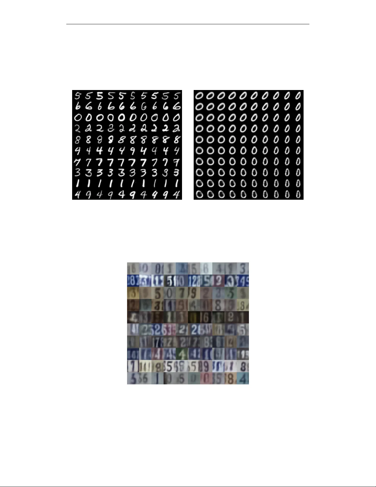
Under revie w as a conference paper at ICLR 2017 D E E P U N S U P E R V I S E D C L U S T E R I N G W I T H G AU S S I A N M I X T U R E V A R I A T I O NA L A U T O E N C O D E R S Nat Dilokthanakul 1 , ∗ , Pedr o A. M. Mediano 1 , Marta Garnelo 1 , Matthew C. H. Lee 1 , Hugh Salimbeni 1 , Kai Arulkumaran 2 & Murray Shanahan 1 1 Department of Computing, 2 Department of Bioengineering Imperial College London London, UK ∗ n.dilokthanakul14@imperial.ac.uk A B S T R AC T W e study a variant of the v ariational autoencoder model (V AE) with a Gaussian mixture as a prior distribution, with the goal of performing unsupervised clus- tering through deep generati ve models. W e observe that the known problem of ov er-regularisation that has been sho wn to arise in regular V AEs also manifests itself in our model and leads to cluster degenerac y . W e show that a heuristic called minimum information constraint that has been shown to mitigate this ef- fect in V AEs can also be applied to improv e unsupervised clustering performance with our model. Furthermore we analyse the ef fect of this heuristic and provide an intuition of the various processes with the help of visualizations. Finally , we demonstrate the performance of our model on synthetic data, MNIST and SVHN, showing that the obtained clusters are distinct, interpretable and result in achie ving competitiv e performance on unsupervised clustering to the state-of-the-art results. 1 I N T RO D U C T I O N Unsupervised clustering remains a fundamental challenge in machine learning research. While long- established methods such as k -means and Gaussian mixture models (GMMs) (Bishop, 2006) still lie at the core of numerous applications (Aggarwal & Reddy, 2013), their similarity measures are lim- ited to local relations in the data space and are thus unable to capture hidden, hierarchical dependen- cies in latent spaces. Alternatively , deep generativ e models can encode rich latent structures. While they are not often applied directly to unsupervised clustering problems, they can be used for dimen- sionality reduction, with classical clustering techniques applied to the resulting low-dimensional space (Xie et al., 2015). This is an unsatisfactory approach as the assumptions underlying the di- mensionality reduction techniques are generally independent of the assumptions of the clustering techniques. Deep generativ e models try to estimate the density of observed data under some assumptions about its latent structure, i.e., its hidden causes. They allow us to reason about data in more complex ways than in models trained purely through supervised learning. Howe ver , inference in models with complicated latent structures can be difficult. Recent breakthroughs in approximate inference have provided tools for constructing tractable inference algorithms. As a result of combining differen- tiable models with variational inference, it is possible to scale up inference to datasets of sizes that would not have been possible with earlier inference methods (Rezende et al., 2014). One popular algorithm under this framework is the variational autoencoder (V AE) (Kingma & W elling, 2013; Rezende et al., 2014). In this paper, we propose an algorithm to perform unsupervised clustering within the V AE frame- work. T o do so, we postulate that generativ e models can be tuned for unsupervised clustering by making the assumption that the observ ed data is generated from a multimodal prior distrib ution, and, correspondingly , construct an inference model that can be directly optimised using the reparameter - ization trick. W e also show that the problem of ov er-regularisation in V AEs can severely effect the performance of clustering, and that it can be mitigated with the minimum information constraint introduced by Kingma et al. (2016). 1 Under revie w as a conference paper at ICLR 2017 1 . 1 R E L A T E D W O R K Unsupervised clustering can be considered a subset of the problem of disentangling latent v ariables, which aims to find structure in the latent space in an unsupervised manner . Recent ef forts have mov ed towards training models with disentangled latent v ariables corresponding to dif ferent factors of variation in the data. Inspired by the learning pressure in the ventral visual stream, Higgins et al. (2016) were able to extract disentangled features from images by adding a regularisation coefficient to the lo wer bound of the V AE. As with V AEs, there is also ef fort going into obtaining disentangled features from generativ e adversarial networks (GANs) (Goodfellow et al., 2014). This has been re- cently achieved with InfoGANs (Chen et al., 2016a), where structured latent variables are included as part of the noise vector , and the mutual information between these latent variables and the gen- erator distribution is then maximised as a mini-max game between the two networks. Similarly , T agger (Gref f et al., 2016), which combines iterativ e amortized grouping and ladder netw orks, aims to perceptually group objects in images by iterati vely denoising its inputs and assigning parts of the reconstruction to dif ferent groups. Johnson et al. (2016) introduced a way to combine amortized inference with stochastic variational inference in an algorithm called structured V AEs. Structured V AEs are capable of training deep models with GMM as prior distribution. Shu et al. (2016) in- troduced a V AE with a multimodal prior where they optimize the variational approximation to the standard variational objecti ve sho wing its performance in video prediction task. The work that is most closely related to ours is the stacked generativ e semi-supervised model (M1+M2) by Kingma et al. (2014). One of the main differences is the fact that their prior distri- bution is a neural network transformation of both continuous and discrete variables, with Gaussian and categorical priors respectiv ely . The prior for our model, on the other hand, is a neural network transformation of Gaussian variables, which parametrise the means and variances of a mixture of Gaussians, with categorical variables for the mixture components. Crucially , Kingma et al. (2014) apply their model to semi-supervised classification tasks, whereas we focus on unsupervised clus- tering. Therefore, our inference algorithm is more specific to the latter . W e compare our results against several orthogonal state-of-the-art techniques in unsupervised clus- tering with deep generati ve models: deep embedded clustering (DEC) (Xie et al., 2015), adversar - ial autoencoders (AAEs) (Makhzani et al., 2015) and categorial GANs (CatGANs) (Springenberg, 2015). 2 V A R I AT I O N A L A U T O E N C O D E R S V AEs are the result of combining variational Bayesian methods with the flexibility and scalability provided by neural netw orks (Kingma & W elling, 2013; Rezende et al., 2014). Using v ariational in- ference it is possible to turn intractable inference problems into optimisation problems (W ainwright & Jordan, 2008), and thus expand the set of av ailable tools for inference to include optimisation techniques as well. Despite this, a key limitation of classical variational inference is the need for the likelihood and the prior to be conjugate in order for most problems to be tractably optimised, which in turn can limit the applicability of such algorithms. V ariational autoencoders introduce the use of neural networks to output the conditional posterior (Kingma & W elling, 2013) and thus allo w the v ariational inference objectiv e to be tractably optimised via stochastic gradient descent and stan- dard backpropagation. This technique, kno wn as the reparametrisation trick, was proposed to enable backpropagation through continuous stochastic variables. While under normal circumstances back- propagation through stochastic v ariables would not be possible without Monte Carlo methods, this is bypassed by constructing the latent variables through the combination of a deterministic function and a separate source of noise. W e refer the reader to Kingma & W elling (2013) for more details. 3 G AU S S I A N M I X T U R E V A R I A T I O N A L A U T O E N C O D E R S In regular V AEs, the prior over the latent v ariables is commonly an isotropic Gaussian. This choice of prior causes each dimension of the multi variate Gaussian to be pushed tow ards learning a separate continuous factor of variation from the data, which can result in learned representations that are structured and disentangled. While this allows for more interpretable latent variables (Higgins et al., 2016), the Gaussian prior is limited because the learnt representation can only be unimodal and does 2 Under revie w as a conference paper at ICLR 2017 not allo w for more comple x representations. As a result, numerous e xtensions to the V AE ha ve been dev eloped, where more complicated latent representations can be learned by specifying increasingly complex priors (Chung et al., 2015; Gre gor et al., 2015; Eslami et al., 2016). In this paper we choose a mixture of Gaussians as our prior, as it is an intuiti ve e xtension of the uni- modal Gaussian prior . If we assume that the observed data is generated from a mixture of Gaussians, inferring the class of a data point is equiv alent to inferring which mode of the latent distribution the data point was generated from. While this gives us the possibility to segregate our latent space into distinct classes, inference in this model is non-trivial. It is well known that the reparametrisation trick which is generally used for V AEs cannot be directly applied to discrete v ariables. Sev eral pos- sibilities for estimating the gradient of discrete variables have been proposed (Glynn, 1990; Titsias & L ´ azaro-Gredilla, 2015). Graves (2016) also suggested an algorithm for backpropagation through GMMs. Instead, we show that by adjusting the architecture of the standard V AE, our estimator of the v ariational lo wer bound of our Gaussian mixture variational autoencoder (GMV AE) can be opti- mised with standard backpropagation through the reparametrisation trick, thus keeping the inference model simple. 3 . 1 G E N E R A T I V E A N D R E C O G N I T I O N M O D E L S Consider the generativ e model p β ,θ ( y y y , x x x, w w w , z z z ) = p ( w w w ) p ( z z z ) p β ( x x x | w w w , z z z ) p θ ( y y y | x x x ) , where an observed sample y y y is generated from a set of latent variables x x x , w w w and z z z under the following process: w w w ∼ N (0 , I I I ) (1a) z z z ∼ M ult ( π π π ) (1b) x x x | z z z , w w w ∼ K Y k =1 N  µ µ µ z k ( w w w ; β ) , diag  σ σ σ 2 z k ( w w w ; β )  z k (1c) y y y | x x x ∼ N  µ µ µ ( x x x ; θ ) , diag  σ σ σ 2 ( x x x ; θ )  or B ( µ µ µ ( x x x ; θ )) . (1d) where K is a predefined number of components in the mixture, and µ µ µ z k ( · ; β ) , σ σ σ 2 z k ( · ; β ) , µ µ µ ( · ; θ ) , and σ σ σ 2 ( · ; θ ) are given by neural networks with parameters β and θ , respectiv ely . That is, the observed sample y y y is generated from a neural network observation model parametrised by θ and the contin- uous latent variable x x x . Furthermore, the distribution of x x x | w w w is a Gaussian mixture with means and variances specified by another neural netw ork model parametrised by β and with input w w w . More specifically , the neural network parameterised by β outputs a set of K means µ µ µ z k and K variances σ σ σ 2 z k , giv en w w w as input. A one-hot vector z z z is sampled from the mixing probability π π π , which chooses one component from the Gaussian mixture. W e set the parameter π k = K − 1 to make z z z uniformly distributed. The generative and variational vie ws of this model are depicted in Fig. 1. x x x w w w z z z y y y β θ 1 x x x w w w z z z y y y φ w φ x 1 Figure 1: Graphical models for the Gaussian mixture variational autoencoder (GMV AE) showing the generativ e model (left) and the variational family (right). 3 Under revie w as a conference paper at ICLR 2017 3 . 2 I N F E R E N C E W I T H T H E R E C O G N I T I O N M O D E L The generativ e model is trained with the variational inference objectiv e, i.e. the log-e vidence lower bound (ELBO), which can be written as L E LB O = E q  p β ,θ ( y y y , x x x, w w w , z z z ) q ( x x x, w w w , z z z | y y y )  . (2) W e assume the mean-field variational family q ( x x x, w w w , z z z | y y y ) as a proxy to the posterior which factorises as q ( x x x, w w w , z z z | y y y ) = Q i q φ x ( x x x i | y y y i ) q φ w ( w w w i | y y y i ) p β ( z z z i | x x x i , w w w i ) , where i indexes ov er data points. T o simplify further notation, we will drop i and consider one data point at a time. W e parametrise each v ariational factor with the recognition networks φ x and φ w that output the parameters of the variational distributions and specify their form to be Gaussian posteriors. W e deriv ed the z -posterior , p β ( z z z | x x x, w w w ) , as: p β ( z j = 1 | x x x, w w w ) = p ( z j = 1) p ( x x x | z j = 1 , w w w ) P K k =1 p ( z k = 1) p ( x x x | z j = 1 , w w w ) = π j N ( x x x | µ j ( w w w ; β ) , σ j ( w w w ; β )) P K k =1 π k N ( x x x | µ k ( w w w ; β ) , σ k ( w w w ; β )) . (3) The lower bound can then be written as, L E LB O = E q ( x x x | y y y )  log p θ ( y y y | x x x )  − E q ( w w w | y y y ) p ( z z z | x x x, w w w )  K L ( q φ x ( x x x | y y y ) || p β ( x x x | w w w , z z z ))  − K L ( q φ w ( w w w | y y y ) || p ( w w w )) − E q ( x x x | y y y ) q ( w w w | y y y )  K L ( p β ( z z z | x x x, w w w ) || p ( z z z ))  . (4) W e refer to the terms in the lower bound as the reconstruction term, conditional prior term, w -prior term and z -prior term respectively . 3 . 2 . 1 T H E C O N D I T I O N A L P R I O R T E R M The reconstruction term can be estimated by drawing Monte Carlo samples from q ( x x x | y y y ) , where the gradient can be backpropagated with the standard reparameterisation trick (Kingma & W elling, 2013). The w -prior term can be calculated analytically . Importantly , by constructing the model this way , the conditional prior term can be estimated using Eqn. 5 without the need to sample from the discrete distribution p ( z z z | x x x, w w w ) . E q ( w w w | y y y ) p ( z z z | x x x, w w w ) h K L  q φ x ( x x x | y y y ) || p β ( x x x | w w w , z z z )  i ≈ 1 M M X j =1 K X k =1 p β ( z k = 1 | x x x ( j ) , w w w ( j ) ) K L  q φ x ( x x x | y y y ) || p β ( x x x | w w w ( j ) , z k = 1)  (5) Since p β ( z z z | x x x, w w w ) can be computed for all z z z with one forward pass, the expectation ov er it can be calculated in a straightforw ard manner and backpropagated as usual. The expectation ov er q φ w ( w w w | y y y ) can be estimated with M Monte Carlo samples and the gradients can be backpropagated via the reparameterisation trick. This method of calculating the e xpectation is similar to the mar ginalisation approach of Kingma et al. (2014), with a subtle difference. Kingma et al. (2014) need multiple forward passes to obtain each component of the z -posterior . Our method requires wider output layers of the neural network parameterised by β , but only need one forward pass. Both methods scale up linearly with the number of clusters. 3 . 3 T H E K L C O S T O F T H E D I S C R E T E L A T E N T V A R I A B L E The most unusual term in our ELBO is the z -prior term. The z -posterior calculates the clustering assignment probability directly from the value of x and w , by asking how far x is from each of the cluster positions generated by w . Therefore, the z -prior term can reduce the KL div ergence between the z -posterior and the uniform prior by concurrently manipulating the position of the clusters and the encoded point x . Intuitiv ely , it would try to merge the clusters by maximising the overlap between them, and moving the means closer together . This term, similar to other KL- regularisation terms, is in tension with the reconstruction term, and is expected to be over -powered as the amount of training data increases. 4 Under revie w as a conference paper at ICLR 2017 3 . 4 T H E O V E R - R E G U L A R I S A T I O N P R O B L E M The possible overpo wering effect of the regularisation term on V AE training has been described numerous times in the V AE literature (Bowman et al., 2015; Sønderby et al., 2016; Kingma et al., 2016; Chen et al., 2016b). As a result of the strong influence of the prior, the obtained latent repre- sentations are often overly simplified and poorly represent the underlying structure of the data. So far there hav e been two main approaches to overcome this effect: one solution is to anneal the KL term during training by allo wing the reconstruction term to train the autoencoder network before slowly incorporating the regularization from the KL term (Sønderby et al., 2016). The other main approach in volv es modifying the objectiv e function by setting a cut-off value that removes the ef- fect of the KL term when it is below a certain threshold (Kingma et al., 2016). As we show in the experimental section below , this problem of over -regularisation is also prev alent in the assignment of the GMV AE clusters and manifests itself in large degenerate clusters. While we show that the second approach suggested by Kingma et al. (2016) does indeed alleviate this merging phenomenon, finding solutions to the ov er-regularization problem remains a challenging open problem. 4 E X P E R I M E N T S The main objective of our experiments is not only to ev aluate the accuracy of our proposed model, but also to understand the optimisation dynamics inv olved in the construction of meaningful, differ - entiated latent representations of the data. This section is divided in three parts: 1. W e first study the inference process in a low-dimensional synthetic dataset, and focus in particular on how the over-re gularisation problem af fects the clustering performance of the GMV AE and how to alle viate the problem; 2. W e then e valuate our model on an MNIST unsupervised clustering task; and 3. W e finally show generated images from our model, conditioned on different values of the latent variables, which illustrate that the GMV AE can learn disentangled, interpretable la- tent representations. Throughout this section we make use of the follo wing datasets: • Synthetic data : W e create a synthetic dataset mimicking the presentation of Johnson et al. (2016), which is a 2D dataset with 10,000 data points created from the arcs of 5 circles. • MNIST : The standard handwritten digits dataset, composed of 28x28 grayscale images and consisting of 60,000 training samples and 10,000 testing samples (LeCun et al., 1998). • SVHN : A collection of 32x32 images of house numbers (Netzer et al., 2011). W e use the cropped version of the standard and the extra training sets, adding up to a total of approximately 600,000 images. 4 . 1 S Y N T H E T I C DAT A W e quantify clustering performance by plotting the magnitude of the z -prior term described in Eqn. 6 during training. This quantity can be thought of as a measure of ho w much dif ferent clusters o verlap. Since our goal is to achiev e meaningful clustering in the latent space, we would expect this quantity to go down as the model learns the separate clusters. L z = − E q ( x x x | y y y ) q ( w w w | y y y )  K L ( p β ( z z z | x x x, w w w ) || p ( z z z ))  (6) Empirically , howe ver , we have found this not to be the case. The latent representations that our model conv erges to mer ges all classes into the same lar ge cluster instead of representing information about the dif ferent clusters, as can be seen in Figs. 2d and 3a. As a result, each data point is equally likely to belong to any of clusters, rendering our latent representations completely uninformati ve with respect to the class structure. W e argue that this phenomenon can be interpreted as the result of over -regularisation by the z -prior term. Given that this quantity is driv en up by the optimisation of KL term in the lower bound, 5 Under revie w as a conference paper at ICLR 2017 it reaches its maximum possible v alue of zero, as opposed to decreasing with training to ensure encoding of information about the classes. W e suspect that the prior has too strong of an influence in the initial training phase and drives the model parameters into a poor local optimum that is hard to be driv en out off by the reconstruction term later on. This observation is conceptually very similar to the ov er-regularisation problem encountered in regu- lar V AEs and we thus hypothesize that applying similar heuristics should help alle viate the problem. W e sho w in Fig. 2f that by using the previously mentioned modification to the lower -bound pro- posed by Kingma et al. (2016), we can avoid the over -regularisation caused by the z -prior . This is achiev ed by maintaining the cost from the z -prior at a constant value λ until it exceeds that threshold. Formally , the modified z -prior term is written as: L 0 z = − max( λ, E q ( x x x | y y y ) q ( w w w | y y y )  K L ( p β ( z z z | x x x, w w w ) || p ( z z z ))  ) (7) This modification suppresses the initial ef fect of the z -prior to merge all clusters thus allo wing them to spread out until the cost from the z -prior cost is high enough. At that point its effect is significantly reduced and is mostly limited to merging individual clusters that are overlapping sufficiently . This can be seen clearly in Figs. 2e and 2f. The former sho ws the clusters before the z -prior cost is taken into consideration, and as such the clusters hav e been able to spread out. Once the z -prior is activ ated, clusters that are very close together will be mer ged as seen in Fig. 2f. Finally , in order to illustrate the benefits of using neural networks for the transformation of the distributions, we compare the density observed by our model (Fig. 2c) with a regular GMM (Fig. 2c) in data space. As illustrated by the figures, the GMV AE allows for a much richer, and thus more accurate representations than regular GMMs, and is therefore more successful at modelling non- Gaussian data. (a) Data points in data space (b) Density of GMV AE − 1 . 5 − 1 . 0 − 0 . 5 0 . 0 0 . 5 1 . 0 1 . 5 − 1 . 5 − 1 . 0 − 0 . 5 0 . 0 0 . 5 1 . 0 1 . 5 (c) Density of GMM − 4 − 3 − 2 − 1 0 1 2 3 4 − 4 − 3 − 2 − 1 0 1 2 3 4 5 (d) Latent space, at poor optimum − 6 − 4 − 2 0 2 4 6 − 4 − 3 − 2 − 1 0 1 2 3 4 (e) Latent space, clusters spreading − 4 − 3 − 2 − 1 0 1 2 3 4 5 − 4 − 3 − 2 − 1 0 1 2 3 4 (f) Latent space, at con vergence Figure 2: Visualisation of the synthetic dataset : (a) Data is distributed with 5 modes on the 2 dimensional data space. (b) GMV AE learns the density model that can model data using a mixture of non-Gaussian distrib utions in the data space. (c) GMM cannot represent the data as well because of the restrictiv e Gaussian assumption. (d) GMV AE, howe ver , suffers from ov er-regularisation and can result in poor minima when looking at the latent space. (e) Using the modification to the ELBO (Kingma et al., 2016) allows the clusters to spread out. (f) As the model con verges the z -prior term is activ ated and regularises the clusters in the final stage by mer ging excessiv e clusters. 6 Under revie w as a conference paper at ICLR 2017 0 5 0 1 0 0 1 5 0 2 0 0 E p o c h − 2 . 0 − 1 . 5 − 1 . 0 − 0 . 5 0 . 0 z - p r i o r t e r m (a) z -prior term with normal ELBO 0 5 0 1 0 0 1 5 0 2 0 0 E p o c h − 2 . 0 − 1 . 5 − 1 . 0 − 0 . 5 0 . 0 z - p r i o r t e r m (b) z -prior term with the modification Figure 3: Plot of z -prior term : (a) Without information constraint, GMV AE suffers from over - regularisation as it con ver ges to a poor optimum that merges all clusters together to avoid the KL cost. (b) Before reaching the threshold value (dotted line), the gradient from the z -prior term can be turned off to av oid the clusters from being pulled together (see text for details). By the time the threshold value is reached, the clusters are sufficiently separated. At this point the acti vated gradient from the z -prior term only mer ges very o verlapping clusters together . Even after acti vating its gradient the value of the z -prior continues to decrease as it is over-po wered by other terms that lead to meaningful clusters and better optimum. 4 . 2 U N S U P E RV I S E D I M AG E C L U S T E R I N G W e now assess the model’ s ability to represent discrete information present in the data on an im- age clustering task. W e train a GMV AE on the MNIST training dataset and ev aluate its clustering performance on the test dataset. T o compare the cluster assignments given by the GMV AE with the true image labels we follow the ev aluation protocol of Makhzani et al. (2015), which we summarise here for clarity . In this method, we find the element of the test set with the highest probability of belonging to cluster i and assign that label to all other test samples belonging to i . This is then repeated for all clusters i = 1 , ..., K , and the assigned labels are compared with the true labels to obtain an unsupervised classification error rate. While we observe the cluster degenerac y problem when training the GMV AE on the synthetic dataset, the problem does not arise with the MNIST dataset. W e thus optimise the GMV AE us- ing the ELBO directly , without the need for any modifications. A summary of the results obtained on the MNIST benchmark with the GMV AE as well as other recent methods is shown in T able 1. W e achieve classification scores that are competiti ve with the state-of-the-art techniques 1 , e xcept for adversarial autoencoders (AAE). W e suspect the reason for this is, again, related to the KL terms in the V AE’ s objecti ve. As indicated by Hoffman et al., the key difference in the adversarial autoen- coders objectiv e is the replacement of the KL term in the ELBO by an adversarial loss that allo ws the latent space to be manipulated more carefully (Hoffman & Johnson, 2016). Details of the network architecture used in these experiments can be found in Appendix A. Empirically , we observe that increasing the number of Monte Carlo samples and the number of clusters makes the GMV AE more robust to initialisation and more stable as shown in Fig. 4. If fewer samples or clusters are used then the GMV AE can occasionally conv erge faster to poor local minima, missing some of the modes of the data distribution. 1 It is worth noting that shortly after our initial submission, Rui Shu published a blog post (http://ruishu.io/2016/12/25/gmvae/) with an analysis on Gaussian mixture V AEs. In addition to providing insightful comparisons to the aforementioned M2 algorithm, he implements a version that achiev es compet- itiv e clustering scores using a comparably simple network architecture. Crucially , he shows that model M2 does not use discrete latent variables when trained without labels. The reason this problem is not as severe in the GMV AE might possibly be the more restrictive assumptions in the generativ e process, which helps the optimisation, as argued in his blog. 7 Under revie w as a conference paper at ICLR 2017 T able 1: Unsupervised classification accuracy for MNIST with different numbers of clusters (K) (reported as percentage of correct labels) Method K Best Run A verage Run CatGAN (Springenberg, 2015) 20 90.30 - AAE (Makhzani et al., 2015) 16 - 90.45 ± 2.05 AAE (Makhzani et al., 2015) 30 - 95.90 ± 1.13 DEC (Xie et al., 2015) 10 84.30 - GMV AE (M = 1) 10 87.31 77.78 ± 5.75 GMV AE (M = 10) 10 88.54 82.31 ± 3.75 GMV AE (M = 1) 16 89.01 85.09 ± 1.99 GMV AE (M = 10) 16 96.92 87.82 ± 5.33 GMV AE (M = 1) 30 95.84 92.77 ± 1.60 GMV AE (M = 10) 30 93.22 89.27 ± 2.50 0 20 40 60 80 100 Epoch 0.0 0.2 0.4 0.6 0.8 1.0 Test Accuracy K=10,M=1 K=10,M=10 K=16,M=1 K=16,M=10 Figure 4: Clustering Accuracy with different numbers of clusters (K) and Monte Carlo samples (M) : After only fe w epochs, the GMV AE con ver ges to a solution. Increasing the number of clusters improv es the quality of the solution considerably . 4 . 2 . 1 I M A G E G E N E R A T I O N So far we have argued that the GMV AE picks up natural clusters in the dataset, and that these clusters share some structure with the actual classes of the images. No w we train the GMV AE with K = 10 on MNIST to show that the learnt components in the distribution of the latent space actually represent meaningful properties of the data. First, we note that there are two sources of stochasticity in play when sampling from the GMV AE, namely 1. Sampling w w w from its prior, which will generate the means and variances of x x x through a neural network β ; and 2. Sampling x x x from the Gaussian mixture determined by w w w and z z z , which will generate the image through a neural network θ . In Fig. 5a we explore the latter option by setting w w w = 0 and sampling multiple times from the result- ing Gaussian mixture. Each row in Fig. 5a corresponds to samples from a different component of the Gaussian mixture, and it can be clearly seen that samples from the same component consistently result in images from the same class of digit. This confirms that the learned latent representation contains well differentiated clusters, and exactly one per digit. Additionally , in Fig. 5b we explore the sensitivity of the generated image to the Gaussian mixture components by smoothly varying 8 Under revie w as a conference paper at ICLR 2017 w w w and sampling from the same component. W e see that while z z z reliably controls the class of the generated image, w w w sets the “style” of the digit. Finally , in Fig. 6 we show images sampled from a GMV AE trained on SVHN, showing that the GMV AE clusters visually similar images together . (a) V arying z (b) V arying w Figure 5: Generated MNIST samples : (a) Each row contains 10 randomly generated samples from different Gaussian components of the Gaussian mixture. The GMV AE learns a meaningful generativ e model where the discrete latent variables z correspond directly to the digit values in an unsupervised manner . (b) Samples generated by traversing around w space, each position of w correspond to a specific style of the digit. Figure 6: Generated SVHN samples : Each row corresponds to 10 samples generated randomly from different Gaussian components. GMV AE groups together images that are visually similar . 5 C O N C L U S I O N W e hav e introduced a class of variational autoencoders in which one level of the latent encoding space has the form of a Gaussian mixture model, and specified a generative process that allows 9 Under revie w as a conference paper at ICLR 2017 us to formulate a variational Bayes optimisation objective. W e then discuss the problem of over - regularisation in V AEs. In the context of our model, we show that this problem manifests itself in the form of cluster degeneracy . Crucially , we show that this specific manifestation of the problem can be solved with standard heuristics. W e ev aluate our model on unsupervised clustering tasks using popular datasets and achieving com- petitiv e results compared to the current state of the art. Finally , we show via sampling from the generativ e model that the learned clusters in the latent representation correspond to meaningful fea- tures of the visible data. Images generated from the same cluster in latent space share relev ant high-lev el features (e.g. correspond to the same MNIST digit) while being trained in an entirely unsupervised manner . It is w orth noting that GMV AEs can be stacked by allo wing the prior on w to be a Gaussian mixture distribution as well. A deep GMV AE could scale much better with number of clusters gi ven that it would be combinatorial with regards to both number of layers and number of clusters per layer . As such, while future research on deep GMV AEs for hierarchical clustering is a possibility , it is crucial to also address the enduring optimisation challenges associated with V AEs in order to do so. A C K N O W L E D G M E N T S W e would lik e to acknowledge the NVIDIA Corporation for the donation of a GeForce GTX Titan Z used in our experiments. W e would like to thank Jason Rolfe, Rui Shu and the revie wers for useful comments. Importantly , we would also like to acknowledge that the variational family which we used throughout this version of the paper was suggested by an anon ymous revie wer . R E F E R E N C E S Charu C Aggarwal and Chandan K Reddy . Data clustering: algorithms and applications . CRC Press, 2013. Christopher M Bishop. Pattern recognition and machine learning. 2006. Samuel R Bowman, Luke V ilnis, Oriol V inyals, Andrew M Dai, Rafal Jozefowicz, and Samy Ben- gio. Generating sentences from a continuous space. arXiv pr eprint arXiv:1511.06349 , 2015. Xi Chen, Y an Duan, Rein Houthooft, John Schulman, Ilya Sutske ver , and Pieter Abbeel. Info- gan: Interpretable representation learning by information maximizing generati ve adversarial nets. arXiv pr eprint arXiv:1606.03657 , 2016a. Xi Chen, Diederik P Kingma, T im Salimans, Y an Duan, Prafulla Dhariwal, John Schulman, Ilya Sutske ver , and Pieter Abbeel. V ariational lossy autoencoder . arXiv pr eprint arXiv:1611.02731 , 2016b. J. Chung, K. Kastner, L. Dinh, K. Goel, A. Courville, and Y . Bengio. A Recurrent Latent V ariable Model for Sequential Data. ArXiv e-prints , June 2015. SM Eslami, Nicolas Heess, Theophane W eber , Y uv al T assa, Koray Kavukcuoglu, and Geof frey E Hinton. Attend, infer , repeat: Fast scene understanding with generative models. arXiv pr eprint arXiv:1603.08575 , 2016. PW Glynn. Likelihood ratio gradient estimation for stochastic systems. Communications of the A CM , 33(10):75–84, 1990. Ian Goodfellow , Jean Pouget-Abadie, Mehdi Mirza, Bing Xu, David W arde-Farle y , Sherjil Ozair , Aaron Courville, and Y oshua Bengio. Generativ e adversarial nets. In Advances in Neural Infor- mation Pr ocessing Systems , pp. 2672–2680, 2014. Alex Graves. Stochastic backpropagation through mixture density distributions. arXiv pr eprint arXiv:1607.05690 , 2016. Klaus Greff, Antti Rasmus, Mathias Berglund, T ele Hotloo Hao, J ¨ urgen Schmidhuber, and Harri V alpola. T agger: Deep unsupervised perceptual grouping. arXiv pr eprint arXiv:1606.06724 , 2016. 10 Under revie w as a conference paper at ICLR 2017 Karol Gregor , Ivo Danihelka, Ale x Graves, Danilo Reze nde, and Daan W ierstra. Draw: A recurrent neural network for image generation. In Pr oceedings of The 32nd International Confer ence on Machine Learning , pp. 1462–1471, 2015. I. Higgins, L. Matthey, X. Glorot, A. Pal, B. Uria, C. Blundell, S. Mohamed, and A. Lerchner. Early V isual Concept Learning with Unsupervised Deep Learning. ArXiv e-prints , June 2016. Matthew D. Hoffman and Matthew J. Johnson. Elbo surgery: yet another way to carve up the variational evidence lower bound. W orkshop in Advances in Appr oximate Bayesian Infer ence, NIPS , 2016. Matthew J Johnson, David Duvenaud, Alexander B W iltschko, Sandeep R Datta, and Ryan P Adams. Composing graphical models with neural networks for structured representations and fast infer- ence. arXiv preprint , 2016. Diederik Kingma and Jimmy Ba. Adam: A method for stochastic optimization. arXiv preprint arXiv:1412.6980 , 2014. Diederik P Kingma and Max W elling. Auto-encoding variational bayes. arXiv pr eprint arXiv:1312.6114 , 2013. Diederik P Kingma, Shakir Mohamed, Danilo Jimenez Rezende, and Max W elling. Semi-supervised learning with deep generative models. In Advances in Neural Information Pr ocessing Systems , pp. 3581–3589, 2014. Diederik P Kingma, Tim Salimans, and Max W elling. Improving v ariational inference with in verse autoregressi ve flo w . arXiv preprint , 2016. Y ann LeCun, L ´ eon Bottou, Y oshua Bengio, and P atrick Haffner . Gradient-based learning applied to document recognition. Proceedings of the IEEE , 86(11):2278–2324, 1998. Alireza Makhzani, Jonathon Shlens, Navdeep Jaitly , and Ian Goodfello w . Adversarial autoencoders. arXiv pr eprint arXiv:1511.05644 , 2015. Y uval Netzer , T ao W ang, Adam Coates, Alessandro Bissacco, Bo W u, and Andrew Y Ng. Reading digits in natural images with unsupervised feature learning. 2011. Danilo Jimenez Rezende, Shakir Mohamed, and Daan W ierstra. Stochastic backpropagation and approximate inference in deep generativ e models. arXiv pr eprint arXiv:1401.4082 , 2014. R. Shu, J. Brofos, F . Zhang, M. Ghav amzadeh, H. Bui, and M. Kochenderfer . Stochastic video prediction with conditional density estimation. In Eur opean Conference on Computer V ision (ECCV) W orkshop on Action and Anticipation for V isual Learning , 2016. Casper Kaae Sønderby , T apani Raiko, Lars Maaløe, Søren Kaae Sønderby , and Ole W inther . How to train deep variational autoencoders and probabilistic ladder networks. arXiv pr eprint arXiv:1602.02282 , 2016. Jost T obias Springenberg. Unsupervised and semi-supervised learning with categorical generativ e adversarial networks. arXiv preprint , 2015. Michalis Titsias and Miguel L ´ azaro-Gredilla. Local expectation gradients for black box variational inference. In Advances in Neural Information Pr ocessing Systems , pp. 2638–2646, 2015. Martin J W ainwright and Michael I Jordan. Graphical models, exponential f amilies, and variational inference. F oundations and T rends R  in Machine Learning , 1(1-2):1–305, 2008. Junyuan Xie, Ross Girshick, and Ali Farhadi. Unsupervised deep embedding for clustering analysis. arXiv pr eprint arXiv:1511.06335 , 2015. A N E T W O R K P A R A M E T E R S For optimisation, we use Adam (Kingma & Ba, 2014) with a learning rate of 10 − 4 and standard hyperparameter values β 1 = 0 . 9 , β 2 = 0 . 999 and  = 10 − 8 . The model architectures used in our experiments are sho wn in T ables A.1, A.2 and A.3. 11 Under revie w as a conference paper at ICLR 2017 T able A.1: Neural network architecture models of q φ ( x x x, w w w ) : The hidden layers are shared between q ( x x x ) and q ( w w w ) , except the output layer where the neural network is split into 4 output streams, 2 with dimension N x and the other 2 with dimension N w . W e exponentiate the variance components to keep their value positiv e. An asterisk (*) indicates the use of batch normalization and a ReLU nonlinearity . For con volutional layers, the numbers in parentheses indicate stride-padding. Dataset Input Hidden Output Synthetic 2 fc 120 ReLU 120 ReLU N w = 2, N w = 2 (Exp), N x = 2, N x = 2 (Exp) MNIST 28x28 con v 16x6x6* (1-0) 32x6x6* (1-0) N w = 150, N w = 150 (Exp), 64x4x4* (2-1) 500* N x = 200, N x = 200 (Exp) SVHN 32x32 conv 64x4x4* (2-1) 128x4x4* (2-1) N w = 150, N w = 150 (Exp), 246x4x4* (2-1) 500* N x = 200, N x = 200 (Exp) T able A.2: Neural network architecture models of p β ( x x x | w w w , z z z ) : The output layers are split into 2 K streams of output, where K streams return mean values and the other K streams output variances of all the clusters. Dataset Input Hidden Output Synthetic 2 fc 120 T anh { N x = 2 } 2 K MNIST 150 fc 500 T anh { N x = 200 } 2 K SVHN 150 fc 500 T anh { N x = 200 } 2 K T able A.3: Neural network architectur e models of p θ ( y y y | x x x ) : The network outputs are Gaussian parameters for the synthetic dataset and Bernoulli parameters for MNIST and SVHN, where we use the logistic function to keep value of Bernoulli parameters between 0 and 1. An asterisk (*) indicates the use of batch normalization and a ReLU nonlinearity . For con volutional layers, the numbers in parentheses indicate stride-padding. Dataset Input Hidden Output Synthetic 2 fc 120 ReLU 120 ReLU { 2 } 2 MNIST 200 500* full-con v 64x4x4* (2-1) 32x6x6* (1-0) 28x28 (Sigmoid) 16x6x6* (1-0) SVHN 200 500* full-con v 246x4x4* (2-1) 128x4x4* (2-1) 32x32 (Sigmoid) 64x4x4* (2-1) 12