Known Unknowns: Uncertainty Quality in Bayesian Neural Networks

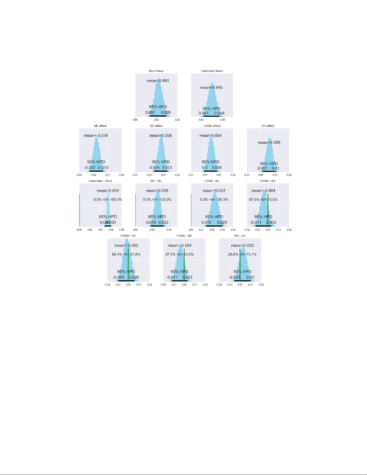
Known Unknowns: Uncertainty Quality in Bayesian Neural Networks Ramon Oliveira ∗ Pedr o T abacof ∗ Eduardo V alle RECOD Lab . — DCA / School of Electrical and Computer Engineering (FEEC) Univ ersity of Campinas (Unicamp) Campinas, SP , Brazil {roliveir, tabacof, dovalle}@dca.fee.unicamp.br Abstract W e ev aluate the uncertainty quality in neural networks using anomaly detection. W e extract uncertainty measures (e.g. entrop y) from the predictions of candidate models, use those measures as features for an anomaly detector , and gauge how well the detector differentiates kno wn from unknown classes. W e assign higher un- certainty quality to candidate models that lead to better detectors. W e also propose a3 novel method for sampling a variational approximation of a Bayesian neural network, called One-Sample Bayesian Approximation (OSB A). W e experiment on two datasets, MNIST and CIF AR10. W e compare the following candidate neural network models: Maximum Likelihood, Bayesian Dropout, OSB A, and — for MNIST — the standard variational approximation. W e sho w that Bayesian Dropout and OSB A provide better uncertainty information than Maximum Likelihood, and are essentially equi valent to the standard variational approximation, but much faster . 1 Introduction While current Deep Learning focuses on point estimates, many real-world applications require a full range of uncertainty . Reliable confidence on the prediction might be as useful as the prediction itself. The debate ov er the dangers of overconfident machine learning has reached the headlines of mass media [ 1 , 2 ]. Indeed, if our models are to driv e cars, diagnose medical conditions, and even analyze the risk of criminal recidivism, unreliable confidence appraisal may ha ve dire consequences. T raditional Deep Learning trains by maximum likelihood — needing aggressiv e regularization to av oid ov erfitting — and only provides point estimates, with limited uncertainty information. If the model outputs a vector of probabilities (as a softmax classifier does), we can quantify its uncertainty using the entropy of the prediction. Howe ver , the model can predict with high confidence for samples way outside the distrib ution seen during training [ 3 ]. Frequentist mitigations, like the bootstrap [ 4 ], do not scale well for deep models. T rue Bayesian models infer the posterior distrib ution ov er all unknown factors, but their computational demands are often prohibiti ve. On the other hand, we may profitably reinterpret under a Bayesian perspectiv e some of the ad hoc regularizations used in ordinary Deep Learning (e.g., dropout [ 5 , 6 ], early stopping [ 7 ], or weight decay [ 8 , 9 ]). Gal and Ghahramani [ 5 ] show that multiple dropout forward passes in test time are equiv alent to a Bayesian prediction (marginalized o ver the parameters’ posteriors) given a particular variational approximation. A more direct (and expensi ve) approach variationally approximates the posterior of each weight [9]. ∗ The first two authors contrib uted equally to this work. W orkshop on Bayesian Deep Learning, NIPS 2016, Barcelona, Spain. 2 One-Sample Bayesian A pproximation (OSB A) Here we propose a nov el Bayesian approach for neural networks, similar to the v ariational approxi- mation of Blundell et al. [ 9 ], but much cheaper computationally . W e call that approach One-Sample Bayesian Appr oximation (OSBA), and in vestigate whether it achie ves better quality of uncertainty information than traditional maximum likelihood. W e use exactly the same approach presented by Blundell et al. ([ 9 ], section 3.2), but instead of sampling the weight matrices for each training example, we sample the matrices only once per mini-batch, and use the same weights for all examples in that mini-batch. That approach leads to the same expected gradient, trading of f higher variance for computational ef ficiency (about 10 times faster with a mini-batch of 100). 3 Uncertainty Quality T o e valuate the quality of uncertainty information, we emplo y anomaly detection: deciding whether or not a test sample belongs to the classes seen during training. More concretely , we pick a classification problem, exclude some classes from training, and use them to e valuate ho w much insight a candidate model has about its o wn classification confidence. W e expect Bayesian neural networks to express such uncertainty well, to the point we can use it to decide whether a sample belongs or not to the kno wn classes. Thus, we employ the A UC of the anomaly detector as a r elative measure of the quality of the uncertainty information output by candidate models (Figure 1). 1. T ra in classifie r 2. Extract unce rtain ty fea tu res from cla ssifier output 3. Use un certa inty fea tu res to train an d test ano maly de tect or ‘8’ 1.2 bit s 1.2 ‘in’ 4. Use de te ctor AUC as measure of unce rtain ty quali ty Figure 1: Uncertainty quality ev aluation using an anomaly detection task. This is the experimental pipeline we follow to compare uncertainty quality among candidate models. (1) W e train a candidate probabilistic classifier for the original task (MNIST or CIF AR10). (2) W e extract uncertainty information from the classifier prediction. (3) W e train a linear anomaly detector using those uncertainty measures as features. (4) W e calculate the A UC of the anomaly detector . Higher detector A UCs indicate that a candidate model provides better uncertainty information. W e contrast two experimental protocols. In the Blind Protocol, we separate the classes into two groups (In and Out); train the candidate neural network using only the In classes; and then train — ov er the In vs. Out classes — a separate anomaly detector using the uncertainty e xtracted from the prediction of the candidate network. In the Calibrated Protocol, we separate the classes into three groups (In, Unknown, and Out); train the candidate network using the In classes with the loss function using the correct labels, and the Unknown classes with the loss function using the equiprobable prediction vector; and then train — ov er the In vs. Out classes — a separate anomaly detector using the same features as before. The test set used to compute the A UC of the anomaly task excludes (obviously) all samples used to train the anomaly detector , and (perhaps less obviously) all samples used to train the candidate neural network. 4 Methodology W e use MNIST [ 10 ] and CIF AR10 [ 11 ] datasets. F or MNIST , the candidate networks ha ve a two- layered fully-connected architecture with 512 neurons each, with dropout of 0.5 applied after each hidden layer . For CIF AR10, the candidate networks ha ve two con volutional blocks (with dropout of 0.25 after each of them), followed by a fully-connected layer with 512 neurons (with dropout of 0.5). W e optimize with ADAM [ 12 ], and limit each training procedure to 100 epochs for MNIST , and 200 2 epochs for CIF AR10. F or each dataset we choose 4 In classes, 4 Out classes, and (for the Calibrated Protocol) 2 Unknown classes (T able 1). W e randomize 20 combinations of In × Out[ × Unknown] classes, with 5 repetitions each, totaling 100 replications. T able 1: Possible combination for In, Out and Unknown classes, showing one sample per class. MNIST’ s classes hav e crisp semantic separation; CIF AR10’ s have considerable overlap due to specialization (e.g., animals) or to background (e.g., sky , lawn, pavement). Such ov erlap might reduce the accuracy of anomaly detection as a measure of uncertainty quality . Dataset In Out Unknown MNIST CIF AR As methods, we ev aluate the usual baseline of Maximum Likelihood (ML), a Bayesian posterior estimated from dropout [ 5 , 13 ] (BD), our approximation for the standard variational Bayesian neural networks using one sample per mini-batch (OSB A), and, for MNIST , we also ev aluate the standard variational approximation [9] (SV). The features for anomaly detection are uncertainty measures extracted from probabilistic predictions. For simplicity , the detector is a linear logistic classifier , with regularization parameter set by stratified cross-validation [ 14 ]. For ML, only the vector of predicted probabilities is av ailable, and thus we employ as feature the entropy — the most theoretically sound measure of uncertainty — over that vector . All Bayesian methods pro vide extra information; we use as feature v ector the av erage and standard deviation of the entropy of the decision vector over 100 network prediction samples (estimating the expectation and variance of the entropy), the entropy of the av erage decision vector ov er those same samples (entropy of estimated expected predictions), and the a verage (ov er classes) of the standard deviations (o ver samples) of the predictions for each class. 4.1 Bayesian ANO V A W e analyze the results using Bayesian ANO V A [ 15 ], with a separate mean for each protocol (Blind vs. Calibrated). That is equi valent to a two-way ANO V A without interactions, where the global mean and experimental protocol f actors are fused together (for interpretability). The methods (ML, BD, OSB A) are the factors of v ariation. W e constrain the sum of the ef fects to be zero, for identifiability . The response v ariable is the A UC of the anomaly detector . W e use weakly informativ e priors. The following model reflects those choices: model = { M L, B D , OS B A } pr otocol = { B lind, C alibr ated } AU C protocol ,model ∼ N ( µ protocol + θ model , σ ) µ protocol ∼ N (0 , 10) θ model ∼ N (0 , σ theta ) σ theta ∼ Half-Cauchy (0 , 10) σ ∼ Half-Cauchy (0 , 10) X i ∈ model θ i = 0 W e implement the model using Stan [ 16 ], and infer the posteriors of the unkno wn parameters using the NUTS algorithm [ 17 ]. T o ensure proper conv ergence, we use 4 chains with 100K steps, including a 10K burn-in, and a thinning factor of 5. From Kruschke’ s suggestion [ 15 ], we present both the distribution of the mar ginal effects, and the distrib ution of the differences between ef fects. 1 1 Code for models, experiments, and analyses at https://github.com/ramon- oliveira/deepstats . 3 5 Results Figure 2: MNIST dataset. Each cell plots the distribution of the influence of the factor sho wn in the label above it, marginalized over all other factors. W e highlight means (expected influence), and 95% Highest Posterior Density interv als (HPD, black bars). On the topmost two rows, we consider the factors themselv es (marginal ef fect), and on the other ro ws, the differences between ef fects. W e consider the dif ferences significant if the HPD does not contain 0.0 (green bar). The domain is the A UC of the anomaly detector . W e sho w the Bayesian ANO V A results in Figures 2 and 3 (for reference, we also sho w the ra w distributions of the A UCs, as boxplots in Figures 4 and 5). Calibration with the auxiliary Unknown classes has a large ef fect, larger than choosing among uncertainty methods. Calibration, howe ver , is not realistic for many applications, due to the artificial constraint of picking well-formatted Unkno wn classes. On the well-controlled scenario pro vided by MNIST , Bayesian methods giv e significantly better uncertainty information than ML. On MNIST , all Bayesian methods outperform ML, and their ef fects do not appear significantly different from each other . On CIF AR10, howe ver , perfect semantic separation between classes is questionable (T able 1), and the performance differences disappear: BD slightly outperforms ML, and OSBA slightly outperforms ML, b ut none of the differences appear significant. T able 2 shows the accuracie s of all candidate models. Note that competing candidate models hav e very similar performance: any gains in anomaly detec tion rather come from enhanced probabilistic information than from increased accuracy . 4 Figure 3: CIF AR10 dataset. Same information and interpretation as Figure 2 above. T able 2: T est accuracy on the original classification task. W e show the mean accuracy , with the standard deviation in parentheses, averaged ov er 100 different replications. Competing candidate models hav e similar accuracies, showing that enhanced uncertainty quality comes from enhanced probabilistic information, not from extra accuracy . Note that OSBA and SV hav e the same accuracy , but the latter is ten times slo wer . Dataset Protocol ML BD OSB A SV MNIST Calibrated 0.990 (0.002) 0.991 (0.002) 0.991 (0.002) 0.991 (0.002) MNIST Blind 0.992 (0.002) 0.992 (0.002) 0.991 (0.002) 0.991 (0.002) CIF AR10 Calibrated 0.878 (0.036) 0.896 (0.033) 0.884 (0.037) — CIF AR10 Blind 0.905 (0.029) 0.908 (0.028) 0.896 (0.032) — 6 Conclusion W e formalized how to ascertain uncertainty quality of neural netw orks by using anomaly detection. W e contrasted the usual maximum likelihood networks to Bayesian alternativ es. Bayesian networks outperformed the frequentist network in all cases. W e also proposed a novel way to sample from a variational approximation of a Bayesian neural network, OSB A, which is much faster than the standard sampling procedure, b ut still retains the same uncertainty quality . OSB A is 10 × faster than SV ; in our experiments, we observ ed relativ e training computational costs of 1 × (ML) to 1 × (BD) to 3 × (OSB A) to 30 × (SV). W e believ e, thus, that techniques like BD and OSB A deserve further in vestigation in more conte xts. Finding a general measure of uncertainty quality is, howe ver , still a challenge. Our experiments suggest that anomaly detection only gives good uncertainty measures for well-separated classes, like MNIST’ s; for uncontrolled datasets like CIF AR10 (or ImageNet), we need a measure that tolerates a degree of semantic intersection between the classes. As future work, we intend to explore other forms of uncertainty quality ev aluation, and to test OSBA in more varied settings. 5 Figure 4: Distributions of the A UCs on MNIST for all combinations of probabilistic approach × experimental protocol. Each boxplot represents 100 replications, obtained by picking at random the In, Out, and (for the calibrated protocol) Unknown classes. Figure 5: Distribution of the A UCs on CIF AR10, obtained the same way as Figure 4 abov e. Acknowledgments W e thank Brazilian agencies CAPES, CNPq and F APESP for financial support. W e gratefully acknowledge the support of NVIDIA Corporation with the donation of the T esla K40 GPU used for this research. Eduardo V alle is partially supported by a Google A wards LatAm 2016 grant, and by a CNPq PQ-2 grant (311486/2014-2). Ramon Oliveira is supported by a grant from Motorola Mobility Brazil. 6 References [1] Jennifer V aughan and Hanna W allach. The inescapability of uncertainty: Ai, uncertainty , and why you should v ote no matter what predictions say . https://medium.com/@jennwv/ uncertainty- edd5caf8981b , 2016. [2] Kate Crawford. Artificial intelligence’ s white guy problem. The New Y ork T imes , 2016. [3] Y arin Gal. Uncertainty in Deep Learning . PhD thesis, Uni versity of Cambridge, 2016. [4] Bradley Efron and Robert J T ibshirani. An introduction to the bootstrap . CRC press, 1994. [5] Y arin Gal and Zoubin Ghahramani. Dropout as a bayesian approximation: Representing model uncertainty in deep learning. arXiv pr eprint arXiv:1506.02142 , 2015. [6] Diederik P Kingma, Tim Salimans, and Max W elling. V ariational dropout and the local reparameterization trick. arXiv pr eprint arXiv:1506.02557 , 2015. [7] Dougal Maclaurin, David Duvenaud, and Ryan P Adams. Early stopping is nonparametric variational inference. arXiv preprint , 2015. [8] Christopher M Bishop. Pattern recognition. Machine Learning , 128, 2006. [9] Charles Blundell, Julien Cornebise, K oray Ka vukcuoglu, and Daan W ierstra. W eight uncertainty in neural network. In Proceedings of The 32nd International Confer ence on Machine Learning , pages 1613–1622, 2015. [10] Y ann LeCun, Corinna Cortes, and Christopher JC Bur ges. The mnist database of handwritten digits, 1998. [11] Alex Krizhe vsky and Geoffre y Hinton. Learning multiple layers of features from tiny images. 2009. [12] Diederik Kingma and Jimmy Ba. Adam: A method for stochastic optimization. arXiv preprint arXiv:1412.6980 , 2014. [13] Y arin Gal and Zoubin Ghahramani. Bayesian conv olutional neural networks with bernoulli approximate variational inference. arXiv preprint , 2015. [14] Payam Ref aeilzadeh, Lei T ang, and Huan Liu. Cross-v alidation. In Encyclopedia of database systems , pages 532–538. Springer , 2009. [15] John Kruschke. Doing Bayesian data analysis: A tutorial with R, J AGS, and Stan . Academic Press, 2014. [16] Bob Carpenter , Andrew Gelman, Matt Hoffman, Daniel Lee, Ben Goodrich, Michael Betan- court, Michael A Brubaker , Jiqiang Guo, Peter Li, and Allen Riddell. Stan: A probabilistic programming language. J Stat Softw , 2016. [17] Matthew D Hoffman and Andrew Gelman. The no-u-turn sampler: adaptiv ely setting path lengths in hamiltonian monte carlo. Journal of Machine Learning Resear ch , 15(1):1593–1623, 2014. 7