Time Series Classification from Scratch with Deep Neural Networks: A Strong Baseline

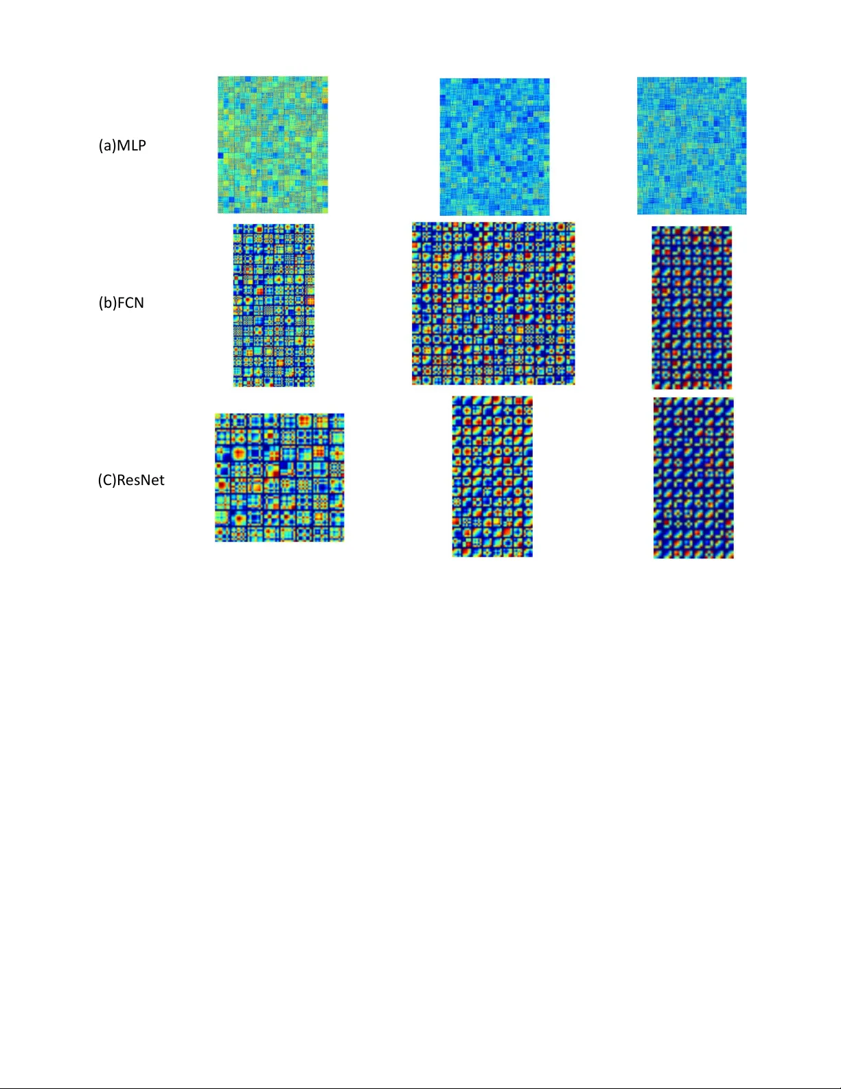
T ime Series Classification from Scratch with Deep Neural Networks: A Strong Baseline Zhiguang W ang, W eizhong Y an GE Global Research { zhiguang.wang, yan } @ge.com T im Oates Computer Science and Electric Engineering Univ ersity of Maryland Baltimore County oates@umbc.edu Abstract —W e propose a simple but strong baseline for time series classification from scratch with deep neural networks. Our proposed baseline models are pur e end-to-end without any heavy prepr ocessing on the raw data or feature crafting. The proposed Fully Convolutional Network (FCN) achieves premium perfor - mance to other state-of-the-art approaches and our exploration of the very deep neural networks with the ResNet structure is also competitive. The global av erage pooling in our conv olutional model enables the exploitation of the Class Activation Map (CAM) to find out the contributing region in the raw data for the specific labels. Our models provides a simple choice f or the real w orld application and a good starting point for the future research. An overall analysis is provided to discuss the generalization capability of our models, lear ned features, network structures and the classification semantics. I . I N T RO D U C T I O N T ime series data is ubiquitous. Both human acti vities and nature produces time series e veryday and ev erywhere, like weather readings, financial recordings, physiological signals and industrial observ ations. As the simplest type of time series data, uni variate time series provides a reasonably good start- ing point to study such temporal signals. The representation learning and classification research has found many potential application in the fields like finance, industry , and health care. Howe v er , learning representations and classifying time se- ries are still attracting much attention. As the earliest baseline, distance-based methods work directly on raw time series with some pre-defined similarity measures such as Euclidean distance or Dynamic time warping (DTW) [1] to perform classification. The combination of DTW and the k-nearest- neighbors classifier is known to be a very ef ficient approach as a golden standard in the last decade. Feature-based methods suppose to extract a set of features that are able to represent the global/local time series patterns. Commonly , these features are quantized to form a Bag-of- W ords (BoW), then giv en to the classifiers [2]. Feature-based approaches mostly differ in the extracted features. T o name a few recent benchmarks, The bag-of-features framework (TSBF) [3] extracts the interv al features with different scales from each interval to form an instance, and each time series forms a bag. A supervised codebook is built with the random forest for classifying the time series. Bag-of-SF A-Symbols (BOSS) [4] proposes a distance based on the histograms of symbolic Fourier approximation words. Its extension, the BOSSVS method [5] combines the BOSS model with the vector space model to reduce the time complexity and improve the performance by ensembling the models with difference window size. The final classification is performed with the One-Nearest-Neighbor classifier . Ensemble based approaches combine different classifiers together to achieve a higher accuracy . Dif ferent ensemble paradigms integrate various feature sets or classifiers. The Elastic Ensemble (PR OP) [6] combines 11 classifiers based on elastic distance measures with a weighted ensemble scheme. Shapelet ensemble (SE) [7] produces the classifiers through the shapelet transform in conjunction with a heterogeneous ensemble. The flat collecti ve of transform-based ensembles (CO TE) is an ensemble of 35 different classifiers based on the features extracted from both the time and frequency domains. All the abo ve approaches need heavy crafting on data preprocessing and feature engineering. Recently , some effort has been spent to exploit the deep neural network, especially con volutional neural networks (CNN) for end-to-end time series classification. In [8], a multi-channel CNN (MC-CNN) is proposed for multiv ariate time series classification. The filters are applied on each single channel and the features are flattened across channels as the input to a fully connected layer . The authors applied sliding windows to enhance the data. The y only ev aluate this approach on two multiv ariate time series datasets, where there is no published benchmark for comparison. In [9], the author proposed a multi-scale CNN approach (MCNN) for univ ariate time series classification. Down sampling, skip sampling and sliding windows are used for preprocessing the data to manually prepare for the multi- scale settings. Although this approach claims the state-of-the- art performance on 44 UCR time series datasets [10], the heavy preprocessing efforts and a large set of hyperparameters make it complicated to deploy . The proposed window slicing method for data augmentation seems to be ad-hoc. W e provide a standard baseline to exploit deep neural networks for end-to-end time series classification without any crafting in feature engineering and data preprocessing. The deep multilayer perceptrons (MLP), fully con v olutional net- works (FCN) and the residual networks (ResNet) are ev aluated on the same 44 benchmark datasets with other benchmarks. Through a pure end-to-end training on the ra w time series data , the ResNet and FCN achiev e comparable or better performance than CO TE and MCNN. The global av erage pooling in our con volutional model enables the exploitation of 500 Input 500 500 Softma x Input Softma x 0.1 0.2 0.2 0.3 R eL U R eL U R eL U 128 BN + R eL U 256 BN + R eL U 128 BN + R eL U Input 64 BN + R eL U 64 BN + R eL U 64 BN + R eL U Global P ooling 128 BN + R eL U 128 BN + R eL U 128 BN + R eL U 128 BN + R eL U 128 BN + R eL U 128 BN + R eL U Softma x Global P ooling + + + (a)M LP (b)F CN (C) R es Ne t Fig. 1. The network structure of three tested neural networks. Dash line indicates the operation of dropout. the Class Activ ation Map (CAM) to find out the contributing region in the raw data for the specific labels. I I . N E T W O R K A R C H I T E C T U R E S W e tested three deep neural network architectures to provide a fully comprehensiv e baseline. A. Multilayer P erceptr ons Our plain baselines are basic MLP by stacking three fully- connected layers. The fully-connected layers each has 500 neurons following two design rules: (i) using dropout [11] at each layer’ s input to improve the generalization capability ; and (ii) the non-linearity is fulfilled by the rectified linear unit (ReLU)[12] as the acti vation function to prev ent saturation of the gradient when the network is deep. The network ends with a softmax layer . A basic layer block is formalized as ˜ x = f dropout,p ( x ) y = W · ˜ x + b h = ReLU ( y ) (1) This architecture is mostly distinguished from the seminal MLP decades ago by the utilization of ReLU and dropout. ReLU helps to stack the networks deeper and dropout largely prev ent the co-adaption of the neurons to help the model generalizes well especially on some small datasets. Ho wev er , if the network is too deep, most neuron will hibernate as the ReLU totally halve the negativ e part. The Leaky ReLU [13] might help, but we only use three layers MLP with the ReLU to provide a fundamental baselines. The dropout rates at the input layer , hidden layers and the softmax layer are { 0.1, 0.2, 0.3 } , respectiv ely (Figure 1(a)). B. Fully Con volutional Networks FCN has shown compelling quality and ef ficiency for se- mantic segmentation on images [14]. Each output pixel is a classifier corresponding to the receptiv e field and the networks can thus be trained pixel-to-pix el given the category-wise semantic segmentation annotation. In our problem settings, the FCN is performed as a feature extractor . Its final output still comes from the softmax layer . The basic block is a conv olutional layer follo wed by a batch normalization layer [15] and a ReLU acti vation layer . The con volution operation is fulfilled by three 1-D kernels with the sizes { 8 , 5 , 3 } without striding. The basic con v olution block is y = W ⊗ x + b s = B N ( y ) h = ReLU ( s ) (2) ⊗ is the con volution operator . W e build the final networks by stacking three conv olution blocks with the filter sizes { 128, 256, 128 } in each block. Unlike the MCNN and MC-CNN, W e exclude any pooling operation. This strategy is also adopted in the ResNet [16] as to prev ent ov erfitting. Batch normalization is applied to speed up the con vergence speed and help improve generalization. After the con volution blocks, the features are fed into a global av erage pooling layer [17] instead of a fully connected layer , which largely reduces the number of weights. The final label is produced by a softmax layer (Figure 1(b)). C. Residual Network ResNet e xtends the neural networks to a v ery deep structures by adding the shortcut connection in each residual block to enable the gradient flo w directly through the bottom layers. It achiev es the state-of-the-art performance in object detection and other vision related tasks [16]. W e explore the ResNet structure since we are really interested to see how the very deep neural networks perform on the time series data. Ob- viously , the ResNet overfits the training data much easier because the datasets in UCR is comparatively small and lack of enough variants to learn the complex structures with such deep networks, b ut it is still a good practice to import the much deeper model and analyze the pros and cons. W e reuse the con volutional blocks in Equation 2 to build each residual block. Let B l ock k denotes the conv olutional block with the number of filters k , the residual block is formalized as h 1 = B l ock k 1 ( x ) h 2 = B l ock k 2 ( h 1 ) h 3 = B l ock k 3 ( h 2 ) y = h 3 + x ˆ h = ReLU ( y ) (3) The number of filters k i = { 64 , 128 , 128 } . The final ResNet stacks three residual blocks and follo wed by a global av erage pooling layer and a softmax layer . As this setting simply reuses the structures of the FCN, certainly there are better structures for the problem, but our giv en structures are adequate to provide a qualified demonstration as a baseline (Figure 1(c)). I I I . E X P E R I M E N T S A N D R E S U L T S A. Experiment Settings W e test our proposed neural networks on the same subset of the UCR time series repository , which includes 44 distinct time series datasets, to compare with other benchmarks. All the dataset has been split into training and testing by default. The only preprocessing in our experiment is z-normalization on both training and test split with the mean and standard deviation of the training part for each dataset. The MLP is trained with Adadelta [18] with learning rate 0.1, ρ = 0 . 95 and  = 1 e − 8 . The FCN and ResNet are trained with Adam [19] with the learning rate 0.001, β 1 = 0 . 9 , β 2 = 0 . 999 and  = 1 e − 8 . The loss function for all tested model is categorical cross entropy . W e choose the best model that achieves the lowest training loss and report its performance on the test set. While this training setting tends to gi ve us a overfitted configuration and most likely to generalize poorly on the test set, we can see that our proposed networks generalize quite well. Unlike other benchmarks, our experiment excludes the hyperparameter tuning and cross v alidation to provide a most unbiased baseline. Such settings also largely reduce the complexity for training and deploying the deep learning models. 1 B. Evaluation T able I shows the results and a comprehensiv e comparison with eight other best benchmark methods. W e report the test error rate from the best model trained with the minimum cross- entropy loss and the number of dataset on which it achie ved the best performance. Some literature (like [9], [5]) also report the ranks and other ranking-based statistics to ev aluate the performance and make the comparison, so we also pro vide the av erage rankings. Howe v er , neither the number of best-performed dataset or the ranking based statistics is an unbiased measurement to compare the performance. The number of best-performed dataset focuses on the top performance and is highly skewed. The ranking based statistics is highly sensitiv e to the model pools. ”Better than” as a comparativ e measurement is also ske wed as the input models might arbitrarily changed. All those ev aluation measures wipe out the factor of number of classes. W e propose a simple ev aluation measure, Mean Per-Class Error (MPCE) to e valuate the classification performance of the specific models on multiple datasets. For a giv en model M = { m i } , a dataset pool D = { d k } with the number of class label C = { c k } and the corresponding error rate E = { e k } , P C E k = e k c k M P C E i = 1 K X P C E k (4) k refers to each dataset and i denotes to each model. The intuition behind MPCE is simple: the expected error rate for a single class across all the datasets. By considering the number of classes, MPCE is more robust as a baseline criterion. A paired T -test on PCE identifies if the differences of the MPCE are significant across different models. C. Results and Analysis W e select se ven existing best methods 2 that claim the state- of-the-art results and published within recent three years: time series based on a bag-of features (TSBF), Elastic Ensemble (PR OP), 1-NN Bag-Of-SF A-Symbols (BOSS) in V ector Space (BOSSVS), the Shapelet Ensemble (SE1) model, flat-CO TE (CO TE) and multi-scale CNN (MCNN). Note that CO TE is an ensemble model which combines the weighted votes over 35 different classifiers. BOSSVS is an ensemble of multiple BOSS models with different windo w length. 1NN-DTW is also included as a simple standard baseline. The training and deploying complexity of our models are small like 1NN-DTW 1 The codes are av ailable at https://github .com/cauchyturing/ UCR Time Series Classification Deep Learning Baseline [20]. 2 ’Best’ means the overall performance is competitive and the model should achiev e the best performance on at least 4 datasets (10% of the all the 44 datasets). T ABLE I T E ST I N G E R RO R A N D T H E M E AN P E R - C L A SS E RR OR ( M PC E ) O N 4 4 U C R T I M E S E R I ES DAT A SE T Err Rate DTW CO TE MCNN BOSSVS PR OP BOSS SE1 TSBF MLP FCN ResNet Adiac 0.396 0.233 0.231 0.302 0.353 0.22 0.373 0.245 0.248 0.143 0.174 Beef 0.367 0.133 0.367 0.267 0.367 0.2 0.133 0.287 0.167 0.25 0.233 CBF 0.003 0.001 0.002 0.001 0.002 0 0.01 0.009 0.14 0 0.006 ChlorineCon 0.352 0.314 0.203 0.345 0.36 0.34 0.312 0.336 0.128 0.157 0.172 CinCECGT orso 0.349 0.064 0.058 0.13 0.062 0.125 0.021 0.262 0.158 0.187 0.229 Coffee 0 0 0.036 0.036 0 0 0 0.004 0 0 0 CricketX 0.246 0.154 0.182 0.346 0.203 0.259 0.297 0.278 0.431 0.185 0.179 CricketY 0.256 0.167 0.154 0.328 0.156 0.208 0.326 0.259 0.405 0.208 0.195 CricketZ 0.246 0.128 0.142 0.313 0.156 0.246 0.277 0.263 0.408 0.187 0.187 DiatomSizeR 0.033 0.082 0.023 0.036 0.059 0.046 0.069 0.126 0.036 0.07 0.069 ECGFiv eDays 0.232 0 0 0 0.178 0 0.055 0.183 0.03 0.015 0.045 FaceAll 0.192 0.105 0.235 0.241 0.152 0.21 0.247 0.234 0.115 0.071 0.166 FaceFour 0.17 0.091 0 0.034 0.091 0 0.034 0.051 0.17 0.068 0.068 FacesUCR 0.095 0.057 0.063 0.103 0.063 0.042 0.079 0.09 0.185 0.052 0.042 50words 0.31 0.191 0.19 0.367 0.18 0.301 0.288 0.209 0.288 0.321 0.273 fish 0.177 0.029 0.051 0.017 0.034 0.011 0.057 0.08 0.126 0.029 0.011 GunPoint 0.093 0.007 0 0 0.007 0 0.06 0.011 0.067 0 0.007 Haptics 0.623 0.488 0.53 0.584 0.584 0.536 0.607 0.488 0.539 0.449 0.495 InlineSkate 0.616 0.551 0.618 0.573 0.567 0.511 0.653 0.603 0.649 0.589 0.635 ItalyPower 0.05 0.036 0.03 0.086 0.039 0.053 0.053 0.096 0.034 0.03 0.04 Lightning2 0.131 0.164 0.164 0.262 0.115 0.148 0.098 0.257 0.279 0.197 0.246 Lightning7 0.274 0.247 0.219 0.288 0.233 0.342 0.274 0.262 0.356 0.137 0.164 MALLA T 0.066 0.036 0.057 0.064 0.05 0.058 0.092 0.037 0.064 0.02 0.021 MedicalImages 0.263 0.258 0.26 0.474 0.245 0.288 0.305 0.269 0.271 0.208 0.228 MoteStrain 0.165 0.085 0.079 0.115 0.114 0.073 0.113 0.135 0.131 0.05 0.105 NonIn vThorax1 0.21 0.093 0.064 0.169 0.178 0.161 0.174 0.138 0.058 0.039 0.052 NonIn vThorax2 0.135 0.073 0.06 0.118 0.112 0.101 0.118 0.13 0.057 0.045 0.049 Oliv eOil 0.167 0.1 0.133 0.133 0.133 0.1 0.133 0.09 0.60 0.167 0.133 OSULeaf 0.409 0.145 0.271 0.074 0.194 0.012 0.273 0.329 0.43 0.012 0.021 SonyAIBORobot 0.275 0.146 0.23 0.265 0.293 0.321 0.238 0.175 0.273 0.032 0.015 SonyAIBORobotII 0.169 0.076 0.07 0.188 0.124 0.098 0.066 0.196 0.161 0.038 0.038 StarLightCurves 0.093 0.031 0.023 0.096 0.079 0.021 0.093 0.022 0.043 0.033 0.029 SwedishLeaf 0.208 0.046 0.066 0.141 0.085 0.072 0.12 0.075 0.107 0.034 0.042 Symbols 0.05 0.046 0.049 0.029 0.049 0.032 0.083 0.034 0.147 0.038 0.128 SyntheticControl 0.007 0 0.003 0.04 0.01 0.03 0.033 0.008 0.05 0.01 0 T race 0 0.01 0 0 0.01 0 0.05 0.02 0.18 0 0 T woLeadECG 0 0.015 0.001 0.015 0 0.004 0.029 0.001 0.147 0 0 T woPatterns 0.096 0 0.002 0.001 0.067 0.016 0.048 0.046 0.114 0.103 0 UW aveX 0.272 0.196 0.18 0.27 0.199 0.241 0.248 0.164 0.232 0.246 0.213 UW aveY 0.366 0.267 0.268 0.364 0.283 0.313 0.322 0.249 0.297 0.275 0.332 UW aveZ 0.342 0.265 0.232 0.336 0.29 0.312 0.346 0.217 0.295 0.271 0.245 wafer 0.02 0.001 0.002 0.001 0.003 0.001 0.002 0.004 0.004 0.003 0.003 W ordSynonyms 0.351 0.266 0.276 0.439 0.226 0.345 0.357 0.302 0.406 0.42 0.368 yoga 0.164 0.113 0.112 0.169 0.121 0.081 0.159 0.149 0.145 0.155 0.142 W in 3 8 7 5 4 13 4 4 2 18 8 A VG Arithmetic ranking 8.205 3.682 3.932 7.318 5.545 4.614 7.455 6.614 7.909 3.977 4.386 A VG geometric ranking 7.160 3.054 3.249 5.997 4.744 3.388 6.431 5.598 6.941 2.780 3.481 MPCE 0.0397 0.0226 0.0241 0.0330 0.0304 0.0256 0.0302 0.0335 0.0407 0.0219 0.0231 as their pipeline is all from scratch without any heavy pre- processing and data augmentations, while our baselines do not need feature crafting. In T able I, we provide four metrics to fully ev aluate dif ferent approaches. FCN indicates the best performance on three metrics at the first sight, while ResNet is also competiti ve on the MPCE score and rankings. In [9], [5], the authors proposed to validate the effecti veness of their models by W ilcoxon signed-rank test on the error rates. Instead, we choose the W ilcoxon rank-sum test as it can deal with the tie conditions among the error rates with the tie correction (Appenix T able II). The p-values in our case are quite dif ferent with the results reported by [9]. Except for MLP and DTW , all other approaches are ’linked’ together based on the p-value. It possibly because the model pool we choose are different and the ranking based statistics is very sensiti ve to the model pool and its size. The MPCE score is reported in the last row . FCN and MLP have the best and worse MPCE score respectively . The ResNet ranks 3rd among all the 11 models, just a little worse than CO TE. A paired T -test of mean on the PCE score is performed to tell if the difference of MPCE is significant (Appendix T able III). Interestingly , we found the difference of MPCE among CO TE, MCNN, BOSS, FCN and ResNet are not significant. These fiv e approaches are clustered in the best group. Analogously , the rest approaches are grouped into Fig. 2. Models grouping by the paired T -test of means on the normalized PCE scores. two clusters based on the T -test results of the MPCE scores (Figure 2). In the best group, BOSS and CO TE are all ensemble based models. MCNN exploit con volutional networks but requires heavy preprocessing in data transformation, do wnsampling and window slicing. Our proposed FCN and ResNet are able to classify time series from scratch and achie ves the premium performance. Compared to FCN, ResNet tends to overfit the data much easier , but is still clustered in the first group without significant dif ference to other four best models. W e also note that the proposed three-layer MLP achie ves comparable results to 1NN-DTW without significant difference. Recent advances on ReLU and dropout work quite well in our experiments to help the MLP gain the similar performance with the previous baseline. I V . L O C A L I Z E T H E C O N T R I B U T I N G R E G I O N S W I T H C L A S S A C T I V A T I O N M A P Another benefit of FCN with the global average pooling layer is its natural extension, the class activ ation map (CAM) to interpret the class-specific region in the data [23]. For a giv en time series, let S k ( x ) represent the activ ation of filter k in the last conv olutional layer at temporal location x . For filter k , the output of the following global average pooling layer is f k = P x S k ( x ) . Let w c k indicate the weight of the final softmax function for the output from filter k and the class c , then the input of the final softmax function is g c = X k w c k X x S k ( x ) = X k X x w c k S k ( x ) W e can define M c as the class activ ation map for class c , where each temporal element is giv en by M c = X k w c k S k ( x ) Hence M c ( x, y ) directly indicates the importance of the activ ation at temporal location x i leading to the classification of a sequence of time series to class c. If the output of the last con volutional layer is not the same as the input, we can still identify the contributing regions most relev ant to the particular category by simply upsampling the class activ ation map to the length of the input time series. In Figure 3, we show two examples of the CAMs output using the abov e approach. W e can see that the discriminative regions of the time series for the right classes are highlighted. W e also highlight the differences in the CAMs for the different labels. The contributing regions for different categories are different. On the ’CBF’ dataset, label 0 is determined mostly by the region where the sharp drop occurs. Sequences with label 1 ha ve the signature pattern of a sharp rise follo wed by a smoothly do wn trending. For label 2, the neural network is address more attention on the long plateau occurs around the middle. The similar analysis is also applied to the contributing region on the ’StarLightCurve’ dataset. Ho wev er , the label 0 and label 1 are quite similar in shapes, so the contrib uting map of label 1 focus less on the smooth trends of drop down while label 0 attract the uniform attention as the signal is much smoother . The CAM provides a natural way to find out the contrib uting region in the raw data for the specific labels. This enables classification-trained con volutional networks to learn to local- ize without any extra effort. Class acti vation maps also allow us to visualize the predicted class scores on any giv en time series, highlighting the discriminative subsequences detected by the conv olutional networks. CAM also provide a way to find a possible explanation on how the conv olutional networks work for the setting of classification. V . D I S C U S S I O N A. Overfitting and Generalization Neural networks is a strong univ ersal approximator which is known to overfit easily due to the large number of param- eters. In our experiments, the overfitting was expected to be significant since the UCR time series data is small and we hav e no validation/test settings, only choose the model with the lowest training loss for test. Howe v er , our models generalize quite well giv en that the training accuracy are almost all 100%. Dropout improves the generalization capability of MLP by a large margin. For the family of con volutional networks, batch normaliza- tion is kno wn to help improve both the training speed and generalization. Another important reason is we replace the fully-connected layer by the global av erage pooling layer before the softmax layer, which greatly reduces the amount of parameters. Thus, starting with the basic network structures without any data transformation and ensemble, our three Label 0: 0.984 Label 1 : 0.999 Label 2 : 0.985 Label 0: 0.822 Label 1 : 0.987 Label 2 : 0.999 high Lo w Fig. 3. The class activ ation mapping (CAM) technique allows the classification-trained FCN to both classify the time series and localize class-specific regions in a single forward-pass. The plots give examples of the contributing regions of the ground truth label in the raw data on the ’CBF’ (above) and ’StarLightCurve’ (below) dataset. The number indicates the likelihood of the corresponding label. models provide very simple but strong baseline for time series classification with the state-of-the-art performance. Another nuance of our results is that, deep neural networks work potentially quite well on small dataset as we expand their generalization by recent adv ances in the network structures and other technical tricks. B. F eature V isualization and Analysis W e adopt the Gramian Angular Summation Field (GASF) [21] to visualize the filters/weights in the neural networks. Giv en a series X = { x 1 , x 2 , ..., x n } , we rescale X so that all values fall in the interval [0 , 1] ˜ x i 0 = x i − min ( X ) max ( X ) − min ( X ) (5) Then we can easily exploit the angular perspective by considering the trigonometric summation between each point to identify the correlation within different time intervals. The GASF are defined as G =  cos( φ i + φ j )  (6) = ˜ X 0 · ˜ X − p I − ˜ X 2 0 · p I − ˜ X 2 (7) I is the unit row vector [1 , 1 , ..., 1] . By defining the inner product < x, y > = x · y − √ 1 − x 2 · p 1 − y 2 and < x, y > = √ 1 − x 2 · y − x · p 1 − y 2 ,GASF are actually quasi-Gramian matrices [ < ˜ x 1 , ˜ x 1 > ] . W e choose GASF because it provides an intuitiv e way to in- terpret the multi-scale correlation in 1-D space. G ( i,j || i − j | = k ) encodes the cosine summation over the points with the striding step k . The main diagonal G i,i is the special case when k = 0 which contains the original values. Figure 4 provides a visual demonstration of the filters in three tested models. The weights from the second and the last layer in MLP are very similar with clear structures and very little degradation occurring. The weights in the first layer , generally , have the higher values than the following layers. The filters in FCN and ResNet are very similar . The con volution extracts the local features in the temporal axis, essentially like a weighted moving average that enhances sev eral receptiv e fields with the nonlinear transformations by the ReLU. The sliding filters consider the dependencies among different time interv als and frequencies. The filters learned in the deeper layers are similar with their preceding layers. This suggests the local patterns across multiple con volutional layers are seemingly homogeneous. Both the visualization and classification performance indicates the effecti veness of the 1- D con volution. C. Deep and Shallow The exploration on the very deep architecture is interesting and informati ve. The ResNet model has 11 layers b ut still holds the premium performance. There are two factors that impact the performance of the ResNet. With shortcut con- nections, the gradients can flo w directly through the bottom (a)M LP (b)F CN (C) R esNe t Fig. 4. V isualization of the filters learned in MLP , FCN and ResNet on the Adiac dataset. For ResNet, the three visualized filters are from the first, second and third conv olution layers in each residual blocks. layers in the ResNet, which largely improv e the interpretability of the model to learn some highly complex patterns in the data. Meanwhile, the much deeper models tend to overfit much easier, requiring more effort in regularizing the model to improv e its generalization ability . In our experiments, the batch normalization and global av erage pooling have largely improved the performance in test data but still tend to ov erfit, as the patterns in the UCR dataset are comparably not so complex to catch. As a result, the test performance of the ResNet is not as good as FCN. When the data is larger and more complex, we encourage the exploration of the ResNet structure since it is more likely to find a good trade-off between the strong interpretability and generalization. D. Classification Semantics The benchmark approaches for time series classification could be categorized into three groups: distance based, feature based and neural neural network based. The combination of distance and feature based approaches are also commonly explored to improve the performance. W e are curious about the classification behavior of dif ferent models as if they all perform similarly on the same dataset, or their feature space and learned classifier are div erged. The semantics of different models are ev aluated based on their PCE scores. W e choose PCA to reduce the dimension because this simple linear transformation is able to preserves large pairwise distances. In Figure 5, the distance between three baseline models with other benchmarks are compar - ativ ely lar ge. which indicates the feature and classification criterion learned in our models are good complement to other models. It is natural to see that FCN and ResNet are quite close with each other . The embedding of MLP is isolated into a single category , meaning its classification behavior is quite different with other approaches. This inspires us that a synthesis of the feature learned by MLP and con volutional networks through a deep-and-wide model [22] might also improve the perfor- mance. V I . C O N C L U S I O N S W e provide a simple and strong baseline for time series classification from scratch with deep neural networks. Our proposed baseline models are pure end-to-end without any Fig. 5. The PCE distribution of different approaches after dimension reduction through PCA. heavy preprocessing on the raw data or feature crafting. The FCN achieves premium performance to other state-of-the- art approaches. Our exploration on the much deeper neural networks with the ResNet structure also gets competitiv e performance under the same experiment settings. The global av erage pooling in our con volutional model enables the ex- ploitation of the Class Activ ation Map (CAM) to find out the contributing region in the raw data for the specific labels. A simple MLP is found to be identical to the 1NN-DTW as the previous golden baseline. An overall analysis is provided to discuss the generalization of our models, learned features, network structures and the classification semantics. Rather than ranking based criterion, MPCE is proposed as an unbiased measurement to ev aluate the performance of multiple models on multiple datasets. Many research focus on time series classification and recent ef fort is more and more lying on the deep learning approach for the related tasks. Our baseline, with simple protocol and small complexity for building and deploy- ing, provides a default choice for the real world application and a good starting point for the future research. R E F E R E N C E S [1] E. Keogh and C. A. Ratanamahatana, “Exact indexing of dynamic time warping, ” Knowledge and information systems , vol. 7, no. 3, pp. 358– 386, 2005. [2] J. Lin, E. Keogh, L. W ei, and S. Lonardi, “Experiencing sax: a novel symbolic representation of time series, ” Data Mining and knowledge discovery , vol. 15, no. 2, pp. 107–144, 2007. T ABLE II A P PE N D I X : T HE P - V A L U ES O F W I LC OX O N R A N K - S U M T E ST B E TW E E N O U R B A SE L I NE M O DE L S W I T H O TH E R A P P ROA CH E S . MLP FCN ResNet DTW 0.7575 0.0203 0.0245 CO TE 0.0040 0.8445 0.8347 MCNN 0.0049 0.9834 0.9468 BOSSVS 0.1385 0.1660 0.1887 PR OP 0.0616 0.2529 0.2360 BOSS 0.0076 0.8905 0.8740 SE1 0.1299 0.0604 0.0576 TSBF 0.1634 0.0715 0.0811 MLP / 0.0051 0.0049 FCN 0.0051 / 0.9169 ResNet 0.0049 0.9169 / [3] M. G. Baydogan, G. Runger, and E. Tuv , “ A bag-of-features framework to classify time series, ” IEEE transactions on pattern analysis and machine intelligence , vol. 35, no. 11, pp. 2796–2802, 2013. [4] P . Sch ¨ afer , “The boss is concerned with time series classification in the presence of noise, ” Data Mining and Knowledge Discovery , vol. 29, no. 6, pp. 1505–1530, 2015. [5] P . Schafer , “Scalable time series classification, ” Data Mining and Knowledge Discovery , pp. 1–26, 2015. [6] J. Lines and A. Bagnall, “Time series classification with ensembles of elastic distance measures, ” Data Mining and Knowledge Discovery , vol. 29, no. 3, pp. 565–592, 2015. [7] A. Bagnall, J. Lines, J. Hills, and A. Bostrom, “T ime-series classification with cote: the collecti ve of transformation-based ensembles, ” IEEE T ransactions on Knowledge and Data Engineering , vol. 27, no. 9, pp. 2522–2535, 2015. [8] Y . Zheng, Q. Liu, E. Chen, Y . Ge, and J. L. Zhao, “Exploiting multi- channels deep conv olutional neural networks for multiv ariate time series T ABLE III A P PE N D I X : T HE P - V A L U ES O F T H E PA I RE D T- TE S T O F T H E M E AN S F O R T H E M P CE S C OR E O N 1 1 B EN C H M AR K M O D E LS . DTW CO TE MCNN BOSSVS PROP BOSS SE1 TSBF MLP FCN ResNet DTW 2.056E-05 5.699E-05 5.141E-02 4.832E-05 2.760E-04 3.040E-03 1.311E-02 4.234E-01 1.451E-04 3.427E-04 CO TE 2.287E-01 3.721E-05 5.911E-03 1.033E-01 1.208E-04 3.528E-04 5.240E-05 3.978E-01 4.351E-01 MCNN 3.652E-04 1.354E-02 2.497E-01 3.634E-03 3.360E-03 8.023E-05 2.495E-01 3.757E-01 BOSSVS 2.140E-01 6.404E-04 1.763E-01 4.335E-01 4.628E-02 2.983E-03 5.067E-03 PR OP 3.739E-02 4.654E-01 1.440E-01 2.061E-02 2.673E-02 4.241E-02 BOSS 2.871E-02 1.759E-02 1.049E-03 1.879E-01 2.751E-01 SE1 1.770E-01 9.901E-03 1.208E-02 3.251E-02 TSBF 7.088E-02 1.510E-03 1.640E-03 MLP 6.832E-05 3.045E-04 FCN 2.508E-01 ResNet classification, ” Fr ontier s of Computer Science , vol. 10, no. 1, pp. 96– 112, 2016. [9] Z. Cui, W . Chen, and Y . Chen, “Multi-scale conv olutional neural net- works for time series classification, ” arXiv preprint , 2016. [10] Y . Chen, E. Keogh, B. Hu, N. Begum, A. Bagnall, A. Mueen, and G. Batista, “The ucr time series classification archive (2015), ” 2016. [11] N. Sriv astav a, G. E. Hinton, A. Krizhevsky , I. Sutske ver , and R. Salakhutdinov , “Dropout: a simple way to prev ent neural networks from overfitting. ” Journal of Machine Learning Research , vol. 15, no. 1, pp. 1929–1958, 2014. [12] V . Nair and G. E. Hinton, “Rectified linear units impro ve restricted boltz- mann machines, ” in Proceedings of the 27th International Confer ence on Machine Learning (ICML-10) , 2010, pp. 807–814. [13] B. Xu, N. W ang, T . Chen, and M. Li, “Empirical evaluation of rectified activ ations in convolutional network, ” arXiv preprint , 2015. [14] J. Long, E. Shelhamer , and T . Darrell, “Fully conv olutional networks for semantic segmentation, ” in Proceedings of the IEEE Confer ence on Computer V ision and P attern Recognition , 2015, pp. 3431–3440. [15] S. Ioffe and C. Szegedy , “Batch normalization: Accelerating deep network training by reducing internal cov ariate shift, ” arXiv preprint arXiv:1502.03167 , 2015. [16] K. He, X. Zhang, S. Ren, and J. Sun, “Deep residual learning for image recognition, ” arXiv preprint , 2015. [17] M. Lin, Q. Chen, and S. Y an, “Network in network, ” arXiv preprint arXiv:1312.4400 , 2013. [18] M. D. Zeiler, “ Adadelta: an adaptiv e learning rate method, ” arXiv pr eprint arXiv:1212.5701 , 2012. [19] D. Kingma and J. Ba, “ Adam: A method for stochastic optimization, ” arXiv preprint arXiv:1412.6980 , 2014. [20] F . Chollet, “Keras, ” https://github .com/fchollet/keras, 2015. [21] Z. W ang and T . Oates, “Imaging time-series to improv e classification and imputation, ” arXiv preprint , 2015. [22] H.-T . Cheng, L. Koc, J. Harmsen, T . Shaked, T . Chandra, H. Aradhye, G. Anderson, G. Corrado, W . Chai, M. Ispir et al. , “W ide & deep learning for recommender systems, ” in Pr oceedings of the 1st W orkshop on Deep Learning for Recommender Systems . A CM, 2016, pp. 7–10. [23] B. Zhou, A. Khosla, A. Lapedriza, A. Oliv a, and A. T orralba, “Learning deep features for discriminative localization, ” arXiv preprint arXiv:1512.04150 , 2015.