Neural Coarse-Graining: Extracting slowly-varying latent degrees of freedom with neural networks

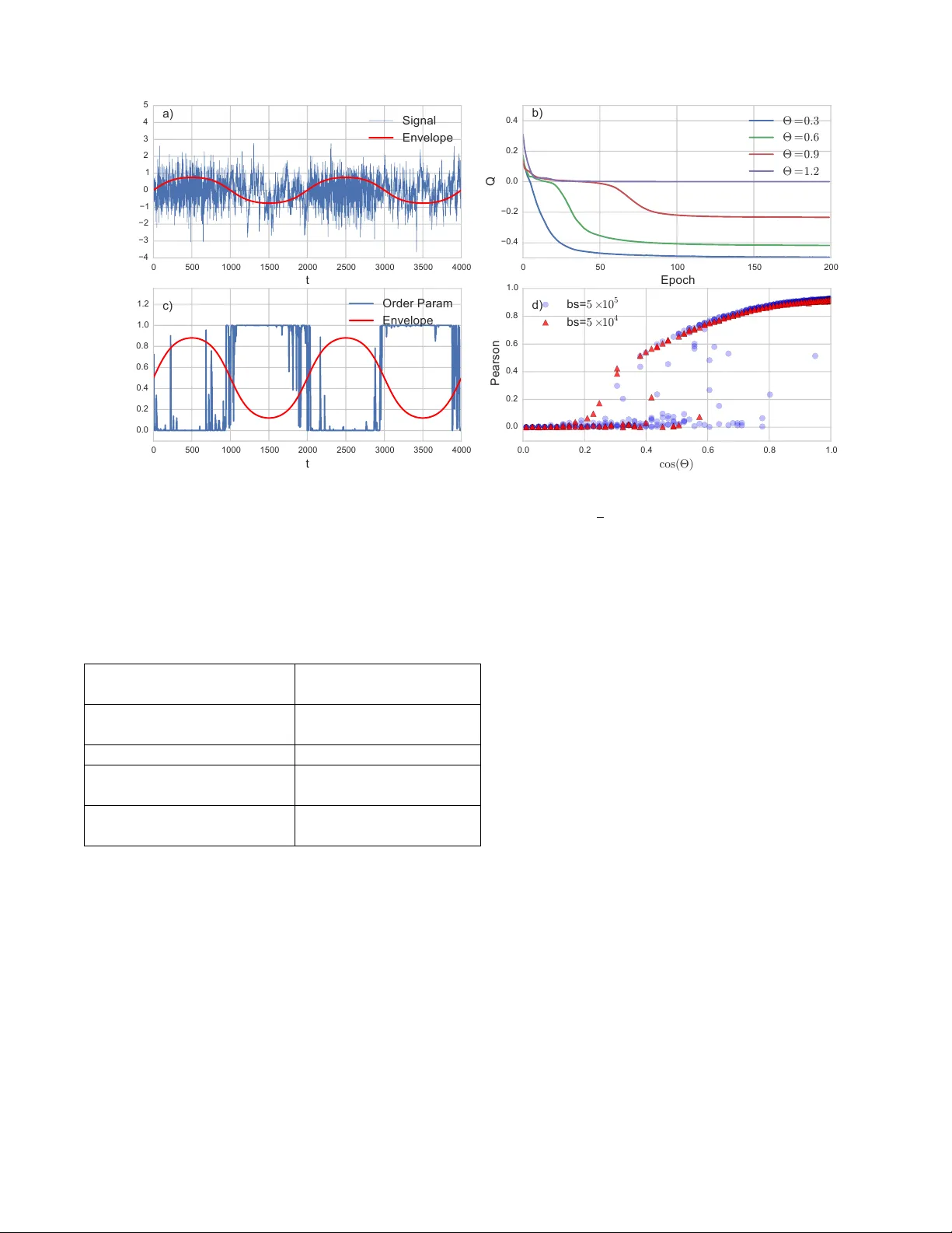
Neural Coarse-Graining: Extracting slo wly-v arying laten t degrees of freedom with neural net w orks Nic holas Gutten b erg Ar aya, T okyo and Earth-Life-Scienc e Institute, T okyo Martin Biehl University of Hertfor dshir e, Hatfield Ry ota Kanai Ar aya, T okyo W e presen t a loss function for neural netw orks that encompasses an idea of trivial versus non- trivial predictions, such that the net w ork join tly determines its own prediction goals and learns to satisfy them. This p ermits the netw ork to c ho ose sub-sets of a problem whic h are most amenable to its abilities to focus on solving, while discarding ’distracting’ elements that in terfere with its learning. T o do this, the net work first transforms the ra w data into a higher-level categorical representation, and then trains a predictor from that new time series to its future. T o preven t a trivial solution of mapping the signal to zero, we introduce a measure of non-trivialit y via a con trast betw een the prediction error of the learned mo del with a naive model of the o verall signal statistics. The transform can learn to discard uninformativ e and unpredictable components of the signal in fav or of the features whic h are b oth highly predictiv e and highly predictable. This creates a coarse-grained mo del of the time-series dynamics, fo cusing on predicting the slo wly v arying laten t parameters whic h con trol the statistics of the time-series, rather than predicting the fast details directly . The result is a semi-sup ervised algorithm whic h is capable of extracting latent parameters, segmenting sections of time-series with differing statistics, and building a higher-lev el representation of the underlying dynamics from unlab eled data. INTR ODUCTION Ho w do physicists do feature engineering? In statistical ph ysics, the corresp onding concept for a ’golden feature’ is that of an order parameter — a single v ariable whic h captures the emergen t large-scale dynamics of the phys- ical system while pro jecting out all of the internal fluc- tuations and microscopic structures. Descriptions based en tirely on a system’s order parameters tend to b e muc h more generalizable and transferable than detailed micro- scopic models, and can capture the behavior of man y dis- parate systems which share some underlying structure or symmetry . The process of extracting out the large-scale dynamics of the system and discarding the microscopic details that are irrelev ant to those o verarc hing dynamics is referred to as ’coarse-graining’. In ph ysical mo dels, one often wan ts to predict dep endencies b etw een parameters or the time evolution of some v ariables, and while work- ing with order-parameters means that the results become m uch more general, it also means that there are certain questions which b ecome unansw erable b ecause the de- tails that the question dep ends on ha v e coarse-grained a wa y . This trade-off go es hand in hand with the abilit y to find order parameters — the intuition is that as one zo oms out to bigger and bigger scales (and, for a physical sys- tem, anything that we in teract with at the h uman lev el of exp erience is extremely zo omed out compared to the atomic scale), certain kinds of mistakes or mismatches b et w een microscopic details of a mo del and realit y will b e erased, while other ones will remain relev ant no mat- ter ho w far y ou zo om out. The order parameters are then the things that are left when you ha ve discarded ev ery- thing that can be efficien tly approximated as you mak e the system bigger. But to perform this in a self-consisten t w ay , one must ask only for those things that matter to the large-scale details, not for anything that could be as- so ciated with some kind of error (b ecause many errors can b e defined, but not all errors will remain relev ant at large scales). If we compare this to the wa y in whic h many problems in machine learning are phrased, there is a no v el element here. Usually , a loss function is designed with a specific problem in mind, and so errors in the p erformance of that problem are de-facto important. But if w e wish to construct an unsup ervised technique, it should someho w decide on its o wn in a w a y inspired on the dep endencies within the data itself what is asymptotically imp ortant and what errors are irrelev an t. F or example, recen t ad- v ances in image synthesis such as st yle transfer use error functions constructed out of intermediate lay er activ a- tions of an ob ject classifier netw ork rather than working at the pixel lev el, with the result of minimizing perceptu- ally meaningful inconsistencies rather than errors in the ra w pixel v alues [1, 2]. So, ho w do y ou find a goo d order parameter? The st yle 2 transfer algorithm effectiv e uses a sup ervised comp onent in order to determine what is and is not meaningful — that is to say , the ob ject classification task whic h pro- vided the aesthetic sense to ev aluate artistic styles (even though the sup ervised task is not directly related). Ev en though the sup ervised task didn’t hav e to b e directly re- lated to the goal of st yle transfer, the details aren’t irrele- v ant — using a net w ork trained to identify the source of a video frame or an auto enco der instead of an ob ject clas- sifier would emphasize certain aspects of the data ov er others. Lab els ab out ob ject t ype and location tend to emphasize edges, whereas delo calized information such as the source video clip of a frame tends to emphasize distributions of color and intensit y ov er specific shap e. Recen t w ork has suggested that it is p ossible to combine generativ e adversarial netw orks and autoenco ders to al- lo w the auto-enco der to effectively disco ver its o wn loss function [3]. Here, an in trinsic predictabilit y is used to driv e the netw ork to organize itself around the data — sp ecifically , the ability to predict whether something is or is not a member of the same distribution as the given data. If w e w ant to do this in an unsup ervised fashion, we need a sense of in trinsic meaningfulness of some features o ver others, using only the data itself as the generator of that meaning. Since w e are considering an approach in whic h it is p ermissible to declare some asp ects of the data irrelev ant, this b ecomes doubly tricky . One thing w e can still do ho w ever is to require that the things w e retain should b e as self-predictive as p ossible. This brings us bac k to the physics analogy — we can ask for degrees of freedom taken from p oint in time which then let us b est predict the future of the data. This kind of approach has b een used to construct things like word2v ec [4] to gener- ate latent conceptual spaces for words. Ho w ever, follo w- ing the analogy from ph ysics, there is a suggestion that p erhaps this is asking for to o m uc h: that is to say , we are trying to predict the future microscopic v ariables from a set of macroscopic measurements, whic h may mean that w e retain information solely for the purp ose of spanning the microscopic basis, and not because it inheren tly ab- stracts and compresses the underlying processes whic h generate the data. F or example, if we w ere to train a word2v ec on a database con taining many different distinct dialects, it w ould b e useful for predicting the ’micro’ future of a sen- tence to know which dialect that sentence b elongs to. But if we wished to model the conceptual structure of sen tences, this dialect information would end up being mostly irrelev an t and w ould force us to learn many par- allel mo dels of the same relationships, muc h in the w ay that a dense neural net w ork has to rep eatedly learn the same relationships at every pixel offset whereas a con vo- lutional net work can kernels which generalize in a trans- lationally inv arian t fashion. This suggests that we may b e able to b etter find go o d Data Encodi ng T 1 T 2 T 1 T 2 T 2 Schmi dhuber , et al (1992) Our method FIG. 1. Relationship b et ween the raw data and the extracted features in Sc hmidhuber et al.[5], v ersus our algorithm. features for data to describ e itself if w e sp ecifically ask for the prop osed features to predict themselves, not ev- erything ab out the data. Doing this allows the learner to in some sense choose its o wn problem to solve, finding those things which can b e efficiently predicted and dis- carding highly unpredictable information from consider- ation. W ork b y Sc hmidhuber, et al.[5] explored this idea b y asking tw o netw orks to make a prediction given dif- feren t views of the data — not requiring them to mak e a ’correct’ prediction, but only to mak e the same prediction — and found that this would organize the net works to disco ver systematic features of the data. W e extend this a bit further and ask for the new representation to con- tain sufficient information on its o wn to predict relation- ships and v ariations of the data in that representation, without specific reference to the underlying data (Fig. 1). What follo ws is a presen tation of a sp ecific algorithm and loss function able to p erform this task in a stable fash- ion, whic h w e will refer to as ’neural coarse-graining’ or ’NCG’. MODEL Loss function The k ey p oin t we use in the analogy to order parame- ters is that an order-parameter should b e self-predictiv e. That is to sa y , the microscopic model contains enough information to predict the future microscopic state, so the macroscopic mo del should retain just enough infor- mation to predict its o wn future macroscopic state (but need not predict the future microscopic state). W e can think of this as tw o separate tasks: one task is to trans- form the data into a new set of v ariables, and the second task is to use those new v ariables at one p oin t to predict the v alue of the new v ariables at a different p oin t. The no vel elemen t is that the prediction is not ev aluated with resp ect to matc hing the ra w data, but is ev aluated with resp ect to matching the transformed data — that is to sa y , the netw ork is helping to define its own loss function 3 (in a restricted w a y). If a v ery slowly v arying v ariable can be found, that would b e fa v ored as prediction (on shorter timescales) b ecomes trivial. This in troduces a potential problem — what if the net- w ork just pro jects all of the data to a constan t v alue? In that case, the predictor w ould be p erfect, but obviously w ouldn’t capture anything about the underlying data. T o a void this, we need the loss function to not just ev aluate the qualit y of the predictions, but also somehow ev alu- ate how hard the task w as that the net w ork set for itself. F or this we take inspiration from information theory and ask, how muc h information is gained ab out the future by making a prediction contingen t up on the past (relative to the stationary statistics of the signal). If we hav e a globally optimal predictor, then this quantit y is kno wn as the predictive information[6], and is defined as: I pred = H( X future ) − H( X future | X past ) where X future represen ts data from a signal ( X t ) t ∈ Z that will b e observed in the future and X past represen ts data already observed in the past. H is the Shannon en tropy . F or a Mark o v c hain the predictive information reduces to: I pred = H( X t +1 ) − H( X t +1 | X t ) In our case, w e consider a transformed signal Y t = f ( X t ) rather than the original signal, and wan t to op- timize that transform to maximize the predictiv e infor- mation of the transformed signal. Since the transform is deterministic this predictiv e information turns out to b e the measure of non-trivial informational closure (NTIC) prop osed by Bertsc hinger et al. [7] (for a deriv ation see App endix NTIC): NTIC = H( Y t +1 ) − H( Y t +1 | Y t ) Because the amount of information gained by condition- ing on the past is b ounded b y the entrop y of the signal b eing predicted, if the transformation maps to a very sim- ple distribution then there will not b e m uch additional information gained by knowledge of the past ev en if the predictor happ ens to be v ery accurate, so this protects against the pro jection on to a constant v alue. If w e only w anted to construct a coarse-grained pro cess whic h is predictiv e of its o wn future and captures as muc h infor- mation as possible about the underlying pro cess then w e could try to optimize f such that NTIC is maximized. Ho wev er, we also wan t to adapt the coarse-graining f to the capabilities of a specific (neural) predictor g whic h giv en y t predicts y t +1 . In that case it can b e b eneficial for the transform f to thro w out information ab out X t whic h in general could be used to increase NTIC. The information that f extracts from X t should then b e just the information that g can predict well. The measure of NTIC do es not accoun t for such an adaptation to g . Nonetheless this can b e done by comparing the v alue predicted by g giv en y t to the v alue y t +1 = f ( x t +1 ) and optimizing for the accuracy of this prediction as w ell as for the capturing of information ab out ( X t ) t ∈ Z . W e note that optimizing b oth f and g b y ev aluating the accuracy of the prediction by g of the actual v alue of y t +1 is a sp ecial case of the state space compression framew ork developed by W olp ert et al. [8]. The nature of the sp ecial case here how ev er requires a com bination of such an accuracy measure with the infor- mation extracting principle of NTIC (see also [9]). While NTIC and the state space compression frame- w ork provide in tuitions for our optimization function the implemen tation employs certain practical tw eaks. The main difference to the previous discussion is that instead of optimizing a function f whic h maps X t to random v ariables Y t w e construct the transforms T 2 suc h that T 2 ( x t ) = s t can b e (and is) directly interpreted as prob- abilit y distribution ov er a macroscopic random v ariable Y t that does not pla y an explicit role itself. In other w ords, we treat s t := T 2 ( x t ) as a probabilit y distribution p ( Y t | x t )(see note [10]) ov er classes of the (implicit) clas- sifier Y . This means s t has as man y comp onen ts as there are classes in the classifier Y . If y denotes such a class then s t ( y ) = T 2 ( x t )( y ) is interpreted as p ( y | x t ). In the same w ay instead of optimizing a specific prediction g we lo ok at the neural transform T 1 ( s t ) = ˆ s t +1 as a proba- bilit y distribution p ( ˆ Y t +1 | s t ). All this allo ws us to k eep the loss function smoothly differen tiable with resp ect to c hanges in the transformation. With this in mind we optimize T 1 and T 2 to minimize: Q ≡ − H( h s t i t ) + h X y ∈ Y s t ( y ) log ˆ s t ( y ) i t where h ... i t indicates an a verage o v er the dataset (for example a time series indexed b y t ). This loss function com bines b oth the optimization of the predictor T 1 (in the form of minimizing the cross-entrop y betw een the true and predicted distribution in the second term) and the av erage en tropy of the transformed signal. The reason for using the en tropy of the dataset a v erage of the s t is that w e don’t wan t T 2 to necessarily map the v arious data points x t to maximum en tropy distributions. Eac h x t ma y well be mapp ed to a delta distribution-lik e s t , instead we w an t T 2 to capture as muc h v ariation from the data as p ossible over time . The cross-entrop y on the other hand should b e small at ev ery p oin t in time which is wh y the time a verage is tak en o v er the instan taneous cross-entropies. The cross- en tropy term tak es the role of the conditional entrop y term in NTIC. Instead of minimizing the rest-entrop y of Y t giv en Y t − 1 w e here minimize the difference b et w een the actually predicted distribution ˆ s t and the observed distribution s t . Ho wev er, the cross-en tropy do es even more than that. 4 Note that we can rewrite the cross-entrop y: X y ∈ Y s t ( y ) log ˆ s t ( y ) = H( s t ) + KL[ s t || ˆ s t ] where KL is the Kullbac k-Leibler div ergence [11]. Since KL-div ergence measures the difference b et ween ˆ s t and s t the en trop y term H( s t ) migh t seem sup erfluous. Ho wev er, it stops s t from b ecoming a uniform distribu- tion. If T 2 w ould map every x t to the uniform distri- bution then a loss function that omits this term (k eep- ing only the KL-divergence from the cross-entrop y term) w ould b e minimized. Due to the entrop y term T 2 is forced to map x t to low entrop y distributions which then, in con- trast to uniform distributions, contain information about the particular x t . The loss function Q can also generalize to partitions of the data other than past and future - any sort of partition could b e used, so long as the same transformation can b e applied to b oth sides of the partition. F or example, rather than predicting the future of a timeseries, one can predict a far-aw ay part of an image given only a lo cal neigh b orho od. The outcome of optimizing against this loss function is that the transform will extract some v ariable sub- comp onen t of the data that the algorithm can b e very confiden t ab out, and to thro w out the rest of the infor- mation in the data. By increasing the num ber of abstract classes or the dimensionality of the regression, this forces the algorithm to include more of the data’s structure in order to maximize the entrop y of the transformed data. Similar considerations go v ern c ho osing this num b er as w ould apply to c ho osing the size of an auto-encoder’s b ottlenec k lay er. Ho wev er, the ordering of learning is opp osite — an autoenco der will start noisy and simplify un til the represen tation fits the bottleneck, whereas this will tend to start simple and then elaborate as it discov- ers more things to ’sa y’ about the data. Some care must b e taken with large n um b ers of classes, as softmax ac- tiv ations experience an increasingly strong tendency to get stuck on the mean as the num ber of classes increases. Metho ds such as hierarc hical softmax [12] or adjusting the softmax temperature o v er the course of training may b e useful to av oid these problems. Arc hitecture In order to construct a concrete implemen tation of neu- ral coarse-graining, the comp onen ts we need are a pa- rameterized transform T 2 from the ra w data into the or- der parameters (the coarse-graining part of the net w ork), and a predictor T 1 whic h uses part of the transformed data to predict other nearby parts. In this pap er, we implemen t both in a single end-to-end connected neural net work. The transform netw ork takes in ra w data, ap- plies an y n umber of hidden la yers, and then has a lay er with a softmax activ ation — this generates the probabil- it y distribution o ver abstract classes which functions as our discov ered order parameter. The netw ork then forks, with one branch simply offsetting the transformed data in time (or space), and the other branch processing the (lo cal) pattern of classes through another arbitrary set of hidden lay ers, finally ending in another softmax la yer. In order to ev aluate the qualit y of the predictions, the output of the final softmax la y er is then compared with the offset output of the intermediate softmax lay er. The most straightforw ard application of NCG is to timeseries analysis, as predicting the future given the presen t provides the needed lo calit y , and sequence to future-sequence means that w e can transform both the inputs and the predicted outputs using the same shared transform. As such, w e examine a few applications of NCG for timeseries analysis and feature engineering, and pro vide a reference Python implementation of NCG using Theano[13] and Lasagne[14] at https://github.com/ arayabrain/neural- coarse- graining/ . TIMESERIES ANAL YSIS - NOISE SEGMENT A TION In man y cases, the observ able data are being generated b y indirectly by some sort of complex pro cess gov erned by a small set of slowly-v arying control parameters. W e can use neural coarse-graining to attempt to discov er these laten t control parameters automatically . F or example, if one had a noise signal where the detailed statistics of the noise were being slowly v aried in the background but the mean of the noise remained constant, a direct attempt to auto-enco de that signal to extract out the hidden feature w ould ha v e difficult y as the auto-encoder would hav e to capture the high entrop y of the noise signal before be- ing able to accurately reproduce amplitude v alues. A self-predictor would b e even worse, as the noise is unpre- dictable in detail. How ever, if one were to first make a new feature which describ ed the high-order statistics of the noise in a lo cal window, then the dynamical b eha vior of that feature might b e highly predictable. W e first consider a problem of this form in or- der to test the ability of neural coarse-graining to ex- tract out the latent con trol parameter in an unsup er- vised fashion. W e generate a timeseries which con- tains a mixture of uncorrelated Gaussian noise and auto- correlated noise, controlled b y an env elop e function ψ = 1 2 (1 + tanh( sin (2 π t/τ ))), where τ controls the timescale (Fig. 3a). W e use τ = 2000 for these exp eriments. Both the indep endent samples and auto correlated noise are c hosen to ha ve zero mean and unit standard deviation. T o generate samples of the auto correlated noise, w e use the finite difference equation x t = cos(Θ) x t − 1 + sin(Θ) η t where η is Gaussian noise with zero-mean and unit standard-deviation. The tw o noise sources are linearly 5 15 7 40 40 1 1 2 Input Signa l T ra nsforme d Signa l 15 7 1 15 7 40 40 1 2 Pred iction Loss T ra nsforme r Pred ictor 50 FIG. 2. Architecture used for the noise segmen tation task. The t wo branches here do not indicate t wo separate net works, but rather the same con volutional op erations applied at t wo differen t p oin ts in time where the offset defines the predic- tion timescale. When computing the loss function, prediction corresp onds to matc hing to a time-shifted v ersion of the trans- formed signal. com bined s t = ψ ( t ) s 1 t + (1 − ψ ( t )) s 2 t to form the signal. W e generate a training set and test set of 5 × 10 5 sam- ples each. An example p ortion of this data is sho wn in Fig. 3a. The transformer and predictor are b oth 1D con volu- tional neural net works with the joint arc hitecture sho wn in Fig. 2. Leaky ReLU activ ations [15] with α = 0 . 05 are used for all la yers except the output of the trans- former and predictor la y ers, which are softmax. Batch normalization [16] is used on the first tw o lay ers of the transformer, and the first tw o lay ers of the predictor. The transformed signal is a probabilit y distribution ov er t wo classes, and the predictor is attempting to predict this distribution 50 timesteps in to the future (this is long enough that the receptive fields of the prediction netw ork do not o v erlap in the input signal). The weigh ts are opti- mized using Adam [17], with a learning rate of 2 × 10 − 3 , and the netw ork is trained for 200 ep o chs. Example con- v ergence curves are shown in (Fig. 3b). T o analyze the p erformance of NCG with resp ect to disco v ering the en- v elop e function w e measure the P earson correlation b e- t ween the transformed signal and the kno wn en velope function ψ . When the correlation length of the auto-correlated noise is long (corresp onding to small Θ), NCG consis- ten tly discov ers an order-parameter that is highly cor- related with the env elope function (Fig. 3c). How ever, as w e decrease the correlation length (increasing Θ), the p erformance drops and the differen t types of noise b e- come less clearly distinguished. At a certain p oint, the outcome of training becomes bistable, either finding a w eakly correlated order-parameter or falling into a lo cal minim um in whic h the net work fails to detect an ything ab out the data. The size of this bistable region is influ- enced b y the batc h sized used in training — if the batch size corresponds to the en tire training set of 5 × 10 5 , the bistable region extends from cos(Θ) = [0 . 2 , 0 . 8]. How- ev er, when a batc h size of 5 × 10 4 samples is used, the apparen t bistable region shrinks to cos(Θ) = [0 . 2 , 0 . 6] (Fig. 3d). In terms of other hyperparameters, the pre- diction distance and learning rate do not seem to mak e m uch difference in the ability of the net work to discern b et w een the t ypes of noise. Increasing the size of the hid- den lay ers lik ewise has very little effect. How ev er, larger filter sizes in the transformer netw ork do app ear to hav e an effect, impro ving the Pearson correlation in large Θ cases. Even at a larger filter size, how ev er, the bistable region app ears to b e unaffected. W e perform a similar test in the case of distinguish- ing b et ween uncorrelated noise drawn from structurally differen t distributions. W e compose signals which alter- nate b et ween Gaussian noise and v arious kinds of dis- crete noise with the same standard deviation and zero mean. This discrete noise is tak en as a generalization of the Bernoulli distribution, suc h that we ha v e some n umber n of discrete v alues whic h are selected from uni- formly . W e consider binary noise ( n = 2, selecting b e- t ween − 1 and 1), balanced ternary noise (selecting from − p 3 / 2 , 0 , p 3 / 2), and un balanced ternary noise (select- ing from − 1+ √ 3 2 , √ 3 − 1 2 , and 1). Whereas a linear autore- gressiv e mo del can distinguish betw een the noise types in the previous case, the different noise distributions in this problem can only be distinguished b y functions that are nonlinear in the signal v ariable, and so this poses a test as to whether that kind of higher-order nonlinear order parameter can b e learned by the net work. In fact, this type of problem does seem to be signifi- can tly harder for NCG to solv e. When the batc h size is the full training set, the net w ork appears to easily b e- come stuc k in a local minimum. As no linear features can distinguish these noise t yp es, the netw ork must find a promising w eakly nonlinear feature b efore it can be- gin to train the predictor successfully . If the batch size is v ery large, the tendency is to simply deca y to wards a v ery safe uniform prediction. How ever, when the batc h size is smaller, fluctuations are larger and hav e a greater c hance of follo wing a spurious linear feature far enough to disco ver a relev ant nonlinearit y . As a result, with smaller batc h size the netw ork is able to find an order parame- ter in the binary noise case. F urthermore, b y decreasing the filter sizes (and correspondingly , putting more em- phasis on deep compositions rather than wide comp osi- 6 0 500 1000 1500 2000 2500 3000 3500 4000 t −4 −3 −2 −1 0 1 2 3 4 5 a) Signal Envelope 0 50 100 150 200 Epoch −0.4 −0.2 0.0 0.2 0.4 Q b) £ = 0 : 3 £ = 0 : 6 £ = 0 : 9 £ = 1 : 2 0 500 1000 1500 2000 2500 3000 3500 4000 t 0.0 0.2 0.4 0.6 0.8 1.0 1.2 c) Order Param Envelope 0.0 0.2 0.4 0.6 0.8 1.0 c o s ( £ ) 0.0 0.2 0.4 0.6 0.8 1.0 Pearson d) b s = 5 £ 1 0 5 b s = 5 £ 1 0 4 FIG. 3. a) Example signal from the correlated noise segmen tation task. The blue line is the ra w signal, the red line is the en velope function b et ween the tw o t ypes of noise. F or this example, cos(Θ) = √ 3 / 2. b) T raining curv es of the loss function for differen t Θ v alues. When the problem becomes hard, sometimes NCG gets stuck in a lo cal minim um around the trivial prediction of assigning all transformed classes equal probability for each point in time. This trivial prediction has a loss of exactly 0, so a plateau around 0 is a common feature of training NCG when the problem is difficult. c) Discov ered coarse-grained v ariable (order parameter) versus the actual env elope function for the ab ov e example. d) P earson correlations b etw een the disco vered coarse-grained v ariable and the true env elope function for m ultiple runs at different Θ v alues. There is an apparent phase transition b ey ond which the net work can no longer solve this problem and segment the noise types. Noise Type Filter sizes P earson Correlation Batc h 5 × 10 4 Batc h 5 × 10 5 Correlated (Θ = 0 . 9) 15-7-1 0.75 0.76 25-7-1 0.82 0.84 Binary 15-7-1 0.86 0.008 Balanced T ernary 15-7-1 0.0003 0.002 3-1-1 0.003 0.008 Un balanced T ernary 15-7-1 0.001 0.0002 3-1-1 0.64 0.14 T ABLE I. Results of neural coarse-graining with different fil- ter sizes and batc h sizes for the different noise segmentation test problems. tions), the netw ork becomes able to solve the un balanced ternary noise case as w ell. TIMESERIES ANAL YSIS - UCI HAR Next, we wan t to test whether the features gener- ated by NCG ha ve an y practical v alue in other machine learning pip elines beyond just b eing a descriptive or ex- ploratory to ol. F or this, w e apply it to the problem of detecting different types of activit y using accelerometer data. In this general class of problem, there is a time- series from one or more accelerometers b eing worn by an individual, and the goal is to categorize what that p erson is doing using a few seconds of that data. The UCI Human Activit y Recognition dataset [18] already con tains a num ber of hand-designed features describ- ing the statistics of the accelerometer data — 2-second long ch unks of the raw data are transformed in to a 516- dimensional representation, taking in to account measures suc h as the standard deviation and kurtosis of fluctu- ations in the raw signal. Using these engineered fea- tures, an out-of-the-b o x application of AdaBo ost achiev es 93.6% accuracy[19]. F or this dataset, we transform a neighborho o d of 7 timesteps of the full 516-dimensional i nput in to 20 classes at the same temporal resolution. The prediction net w ork tak es as input a size 5 neigh borho o d of the transformed classes and predicts the class at 20 steps in to the future. That is to say , the full receptiv e field of the predictor extends from t − 4 to t + 4 to predict the class at t + 20 (whic h itself dep ends directly on nothing earlier than t + 17). The net w ork uses leaky ReLU with α = 0 . 05, batc h 7 T ransformer Con v5-100 30% Drop out Con v3-100 30% Drop out Con v1-20 Softmax Predictor Con v5-100 30% Drop out Con v1-100 30% Drop out Con v1-20 Softmax T ABLE I I. Architecture of the netw ork used for UCI HAR timeseries analysis. All lay ers ha ve batch normalization ap- plied, and Leaky ReLU as the activ ation for the non-softmax la yers. Discovered Category Walking Upstairs Downstairs Sitting Standing Laying Activity 0.0 0.5 1.0 FIG. 4. Correlation matrix betw een the discov ered coarse- grained v ariables and the different activity classes. The columns of the matrix are sorted to bring together coarse- grained v ariables whic h are most strongly correlated with eac h activity in turn. Most of the coarse-grained v ariables are strongly asso ciated with a single activity class, with the exceptions of columns 9, 13, and 20. normalization on each lay er, and 30% drop out b et w een eac h lay er. A schematic of the full arc hitecture is given in T able II. The data is split into ch unks of length 120 steps, and the net work is trained for 510 ep ochs using Adam optimization with a learning rate of 5 × 10 − 3 . The resulting classes already show strong correlations with the differen t b eha viors (Fig. 4). How ev er, it’s clear that for some samples the discov ered classes are ambigu- ous and do not uniquely iden tify the b ehavior. When w e use these new features from three adjacen t timesteps with AdaBo ost (in the form of Scikit-Learn’s Gradien t- Bo ostingClassifier implementation [20]) on their own, we observ e only 87.4% accuracy on the test set, compared with 93.7% using the original features. Ho wev er, when w e com bine the original features with our classes, the accuracy on the test set increases to 95.2%. So the new features seem to exp ose some structures in the data which are otherwise more difficult to extract b y AdaBo ost itself. One confounding factor here is that our algorithm had access to multiple timesteps, whereas the only temporal information a v ailable to the original score w as from the 2-second interv al used to produce the hand-designed fea- tures in the original data. As such, it may be that this increase in p erformance is only due to the a v ailability of a wider time windo w of inputs. W e test this b y measuring the p erformance using the original features, but taken at t − 8, t , and t + 8 in order to appro ximate the range of ac- cess that our algorithm w as provided. This impro v es the p erformance as well, resulting in 94.6% accuracy on the F eatures Accuracy Original (1 fr.) 93.7 Original (3 fr.) 94.6 NCG (3 fr.) 87.4 NCG + Original (1 fr.) 95.6 NCG + Original (3 fr.) 95.1 T ABLE I II. Results of AdaBo ost classifier on the UCI HAR dataset trained with differen t sets of features — the origi- nal features from one or three frames, and the neural coarse- graining features with one or three frames (and in com bina- tion with the original features). The NCG features pro duce a worse classifier on their o wn, but result in an improv ement o ver the original features alone when combined. test set. How ev er, when w e tak e the time-extended orig- inal features and combine with our discov ered features, the performance is worse than just using the instanta- neous original features with our classes (95.1%). This seems to suggest that some degree of what the discov ered order parameters are doing is to efficien tly summarize co- heren t asp ects of the time-dependence of the data. W e can also use the classes generated by neural coarse- graining to do exploratory analyses of the data. Since the transformed data tends to b e locally stable with sharp transitions b et w een the categories, a natural thing to do is to sample the b et ween-class transitions as a Marko v pro cess. F or the UCI HAR dataset there’s a complica- tion — the data was taken according to a sp ecific proto- col, ordering the activities to be p erformed in a specific w ay for each sub ject. The length of time spent on eac h activit y is quite short, so it would b e hard to make pre- dictions that did not cross some activity b oundary . It turns out that our algorithm ends up predominantly dis- co vering this structure in the resulting Mark o v pro cess (Fig. 5). The regularity of the proto col means that dis- co vering what activity is curren tly under w ay is a very go od predictor of what activity will be taking place in the future, and as suc h probably strongly encouraged the or- der parameters to b e correlated with the activit y t yp es. The double-lo op structure may indicate the discov ery of some sub ject-specific details. CONCLUSIONS W e ha v e introduced the neural coarse-graining algo- rithm, whic h extracts coarse-grained features from a set of data which are b oth readily determined from the lo cal details, and whic h also are highly predictive of them- selv es. The coarse-graining do es not preserv e all under- lying relationships from the data, but instead tries to find some subset of those relationships which it can most readily predict. This provides a form of unsup ervised la- b elling, to map a problem on to a simpler sub-problem that discards the parts of the data whic h confound pre- 8 FIG. 5. Left: Graph of the transitions betw een discov ered categories in the transformed data. Links are drawn for tran- sitions which occur with ov er a 20% probabilit y from the pre- vious class. The n umbering of nodes in this plot corresp onds to the column order in Fig. 4. No de colors are based on the corresp onding highly-correlated activit y . Right: Graph of the transitions b etw een activities in the raw data. The activities w ere alw a ys p erformed in a fixed order, so this cyclic structure ends up strongly determining the b ehavior of long-term tem- p oral sequence predictions — p ossibly an artefact that NCG is picking up on in generating its features for this problem. diction. One adv an tage of this approach compared to directly using self-prediction on the underlying data is that neural coarse-graining is free to predict parameters con trolling the distribution of the noise rather than the details of the individual random samples, making this metho d more robust to prediction tasks on highly noisy data sets, including ones where the structure of the noise ma y b e imp ortant to understand or tak e into account. Although neural coarse-graining trains a predictor, it is unclear whether in general the predictor itself is useful to- w ards any particular task. Rather, it is the wa y in which needing to b e able to construct a predictor forces the transformation to preserve certain features of the data o ver others. As suc h, the sub-problem that the netw ork decides to solv e can be used for exploratory analysis to c haracterize the dominan t features of the underlying pro- cesses behind a set of data. By examining the transition matrix betw een disco vered classes, it is possible to ex- tract a coarse-grained picture of the dynamics, detecting things such as underlying perio dicities or branc hing de- cision points in time-series data. In addition, from our exp erimen ts on UCI HAR, it seems that the extracted features ma y capture or clean up details of the under- lying data in a w ay that can be used to augmen t the p erformance of other machine learning algorithms — a form of unsup ervised feature engineering. A CKNOWLEDGMENTS Martin Biehl would like to thank Nathaniel Virgo and the ELSI Origins Netw ork (EON) at the Earth-Life- Science Institute (ELSI) at T okyo Institute of T ec hnol- ogy for inviting him as a short-term visitor. P art of this researc h was performed during that sta y . App endix: NTIC W e show that optimizing non-trivial informational clo- sure reduces to optimizing I pred of the transformed sig- nal. In general if w e ha ve tw o processes ( X t ) t ∈ Z and ( Y t ) t ∈ Z and w e assume that the join t pro cess ( X t , Y t ) t ∈ Z is a Mark o v c hain then non-trivial informational closure of ( Y t ) t ∈ Z with resp ect to ( X t ) t ∈ Z is measured by (at an y time t ): NTIC := I( X t : Y t +1 ) − I( Y t +1 : X t | Y t ) . (A.1) The smaller this v alue the more non-trivially closed is Y t . The first term measure how muc h information is con- tained in X ab out the future of Y . The second term measure how m uc h more information X contains about the future of Y than is already contained in the present of Y . The process Y is called non-trivially closed with resp ect to X b ecause it shares information with X but this information is contained in Y itself. In our case Y t = f ( X t ) where f is a deterministic trans- form. Therefore the second term in Eq. A.1 reduces to I( Y t +1 : X t | Y t ) = H( f ( X t +1 ) | f ( X t )) − H( f ( X t +1 ) | X t ) . (A.2) W riting the first term also via the en tropies w e can easily see that NTIC = H( f ( X t +1 )) − H( f ( X t +1 ) | f ( X t )) . (A.3) This is just the Mark o v chain appro ximation of I pred of ( Y t ) t ∈ Z . App endix: Contin uous order parameters When constructing things in terms of information mea- sures, it is easier to use discrete states rather than con- tin uous states. Ho wev er, a con tinuous version of the coarse-graining loss function can b e constructed to ex- tract con tinuous-v alued v ariables. The interpretation of these is a bit simpler, as it do esn’t require treating the transformed v ariable as a distribution and as a v alue in different parts of the algorithm. In order to make this construction, w e m ust b e able to compare the en- trop y of the transformed signal from a naive point of 9 view with the en trop y of the transformed signal condi- tioned on the predictor. T o do this, we generate t wo sig- nals: the signal corresp onding to the coarse-grained v ari- able y ( t ) and the ’residual’ signal corresponding to the prediction error against the future coarse-grained signal  ≡ P ( y ( t + ∆) | y ( τ < t )) − y ( t + ∆). W e then construct a loss function which measures the difference in en tropies b et w een y ( t ) and  ( t ). T o do so, we must assume something ab out the dis- tributions of y and  . If we assume that these signals corresp ond to samples taken from a multi-dimensional Gaussian distribution, then the entrop y of each signal corresp onds to the logarithm of the determinan t of the co v ariance matrix. This lets us construct a regression loss function for contin uous coarse-grained v ariables. Q reg ≡ log( det co v( y , y ) det co v( ,  ) ) , W e mostly include this example for completeness and as a demonstration of how to construct coarse-graining loss functions for differen t types of v ariable. Although this form may be conceptually more tidy than the dis- crete case, we hav e found that in general the discrete v ersion of this algorithm seems to perform better and is less prone to o verfitting, at least in those cases whic h w e ha ve inv estigated. [1] L. A. Gatys, A. S. Eck er, and M. Bethge, arXiv preprint arXiv:1508.06576 (2015). [2] J. Johnson, A. Alahi, and L. F ei-F ei, arXiv preprint arXiv:1603.08155 (2016). [3] A. B. L. Larsen, S. K. Sønderby , and O. Winther, arXiv preprin t arXiv:1512.09300 (2015). [4] T. Mikolo v and J. Dean, Adv ances in neural information pro cessing systems (2013). [5] J. Schmidh uber and D. Prelinger, Neural Computation 5 , 625 (1993). [6] W. Bialek and N. Tishb y , arXiv preprint cond- mat/9902341 (1999). [7] N. Bertschinger, E. Olbrich, N. Ay , and J. Jost, in Ex- plor ations in the c omplexity of p ossible life : abstr acting and synthesizing the principles of living systems - Pr o- c e e dings of the 7th German Workshop on A rtificial Life (Jena, 2006) pp. 9–19. [8] D. H. W olp ert, J. A. Gro c how, E. Libby , and S. DeDeo, CoRR abs/1409.7403 (2014). [9] In the notation of [8] that pap er let Y = Y , O = π = f , φ = g , and ρ = I d . Then the accuracy costs they prop ose (e.g. in their Eqs. (4) and (11)) are similar to our term for prediction accuracy . How ever b ecause the observ able O w e wan t to learn about here is the same as the map π (our f ) to the macroscopic state that w e are optimizing this accuracy cost is not enough. In contrast to the usual ap- plication of the state space compression framew ork where O is externally determined here the optimization can just c ho ose π to map every state to a constan t. This would alw ays result in high accuracy . F or this reason our accu- racy cost has an additional en tropy term similar to the first term in NTIC. [10] Here we use the notation p ( A ) with a capital A to indicate the entire distribution p : A → [0 , 1] with P a ∈A p ( a ) = 1 where A is the set of possible v alues of random v ariable A . [11] The Kullback-Leibler divergence[see e.g. 21] b et ween t wo distribution p, q is defined as KL[ p || q ] := P x p ( x ) log p ( x ) q ( x ) . [12] T. Mikolo v, K. Chen, G. Corrado, and J. Dean, arXiv preprin t arXiv:1301.3781 (2013). [13] Theano Dev elopment T eam, arXiv e-prints abs/1605.02688 (2016). [14] S. Dieleman, J. Sc hlter, C. Raffel, E. Olson, S. K. Snderb y , D. Nouri, D. Maturana, M. Thoma, E. Bat- ten b erg, J. Kelly , J. D. F auw, M. Heilman, D. M. de Almeida, B. McF ee, H. W eideman, G. T akcs, P . de Ri- v az, J. Crall, G. Sanders, K. Rasul, C. Liu, G. F rench, and J. Degra ve, “Lasagne: First release.” (2015). [15] A. L. Maas, A. Y. Hannun, and A. Y. Ng, in Pr o c. ICML , V ol. 30 (2013). [16] S. Ioffe and C. Szegedy , arXiv preprin t (2015). [17] D. Kingma and J. Ba, arXiv preprin t (2014). [18] D. Anguita, A. Ghio, L. Oneto, X. Parra, and J. L. Rey es-Ortiz, in ESANN (2013). [19] R. F u, Y. Song, and W. Zhao, . [20] F. Pedregosa, G. V aro quaux, A. Gramfort, V. Mic hel, B. Thirion, O. Grisel, M. Blondel, P . Prettenhofer, R. W eiss, V. Dub ourg, J. V anderplas, A. Passos, D. Cour- nap eau, M. Brucher, M. Perrot, and E. Duc hesnay , Jour- nal of Mac hine Learning Research 12 , 2825 (2011). [21] T. M. Co ver and J. A. Thomas, Elements of information the ory (Wiley-Interscience, Hoboken, N.J., 2006).