Asynchronous Stochastic Gradient MCMC with Elastic Coupling

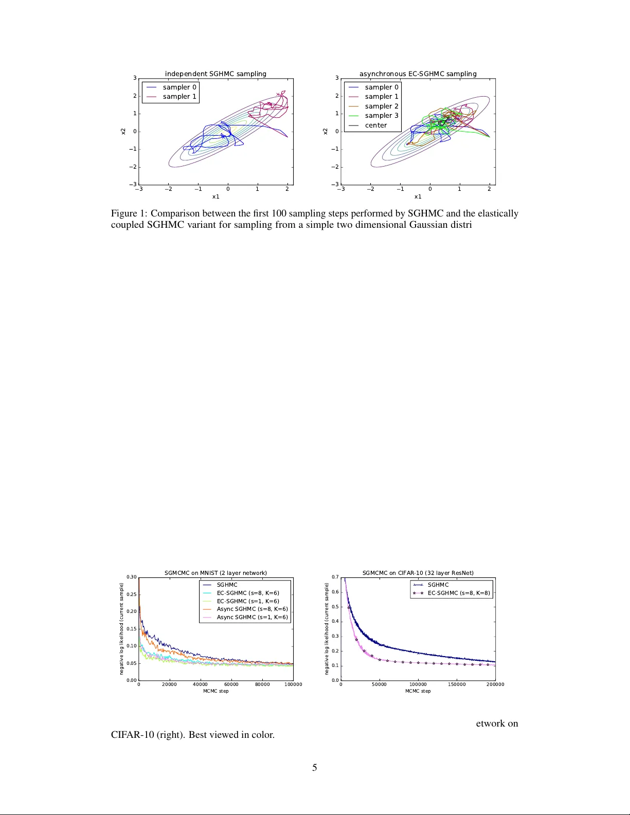
Asynchr onous Stochastic Gradient MCMC with Elastic Coupling Jost T obias Springenberg Aaron Klein Stefan Falkner Frank Hutter Department of Computer Science, Univ ersity of Freib urg {springj,kleinaa,sfalkner,fh}@cs.uni-freiburg.de Abstract W e consider parallel asynchronous Marko v Chain Monte Carlo (MCMC) sampling for problems where we can lev erage (stochastic) gradients to define continuous dynamics which explore the tar get distribution. W e outline a solution strategy for this setting based on stochastic gradient Hamiltonian Monte Carlo sampling (SGHMC) which we alter to include an elastic coupling term that ties together multiple MCMC instances. The proposed strategy turns inherently sequential HMC algorithms into asynchronous parallel versions. First e xperiments empirically sho w that the resulting parallel sampler significantly speeds up exploration of the target distribution, when compared to standard SGHMC, and is less prone to the harmful effects of stale gradients than a nai v e parallelization approach. 1 Introduction and Background Over the last years the ever increasing comple xity of machine learning (ML) models together with the increasing amount of data that is a v ailable to train them has resulted in a great demand for parallel training and inference algorithms that can be deployed over many machines. T o meet this demand, ML practitioners have increasingly relied on (asynchronous) parallel stochastic gradient descent (SGD) methods for optimizing model parameters [Recht et al., 2011, Dean et al., 2012, Zhang et al., 2015]. In contrast to this, the literature on ef ficient parallel methods for sampling from the posterior ov er model parameters given some data is much more scarce. Examples of algorithms for this setting typically are constrained to specific model classes [Ahmed et al., 2012, Ahn et al., 2015, Simsekli et al., 2105] or “only” consider data parallelism [Ahn et al., 2014]; in summary – with the exception of recent work by Chen et al. [2016] – a general sampling pendant of asynchronous SGD methods is missing. In this paper we consider the general problem of sampling from an arbitrary posterior distrib ution ov er parameters θ ∈ R n giv en a set of observed datapoints x ∈ D where we have K machines av ailable to speed up the sampling process. W ithout loss of generality we can write the mentioned posterior as p ( θ |D ) ∝ exp( − U ( θ )) where we define U ( θ ) to be the potential ener gy U ( θ ) = − P x ∈ D log p ( x | θ ) − log p ( θ ) . Many algorithms for solving this problem such as Hamiltonian Monte Carlo [Duane et al., 1987, Neal, 2010] further augment this potential energy with terms depending on auxiliary variables y ∈ R A to speed up sampling. In this more general case we write the posterior as p ( z |D ) ∝ exp( − H ( z )) , where z = [ θ , y ] ∈ R m denotes the collection of all variables and H ( z ) denotes the Hamiltonian H ( z ) = H ( θ, y ) = U ( θ ) + g ( θ , y ) . Samples from p ( θ |D ) can then be obtained by sampling from p ( z |D ) and discarding y if we additionally assume that marginalizing out y from p ( z |D ) results only in a constant offset c ; that is we require R y ∈ R A exp( − g ( θ , y )) d y = c . 1.1 Stochastic Gradient Hamiltonian Monte Carlo Stochastic gradient MCMC (SGMCMC) algorithms solve the abov e described sampling problem by assuming access to a – possibly noisy – gradient of the potential U ( θ ) with respect to parameters θ . In this case – assuming properly chosen auxiliary variables – sampling can be performed via an analogy to physics by simulating a system based on the Hamiltonian H ( z ) . More precisely , follo wing the general formulation from Ma et al. [2015], one can simulate a stochastic differential equation (SDE) of the form d z = f ( z ) d t + p 2 D ( z ) d w t , (1) where f ( z ) : R m → R m denotes the deterministic drift incurred by H ( z ) , D ( z ) : R m → R m × R m is a diffusion matrix, the square root is applied element-wise, and w t ∈ R m denotes Brownian motion. Under fairly general assumptions on the functions f and D the unique stationary distribution of this system is equi v alent to the posterior distrib ution p ( θ |D ) . Specifically , Ma et al. [2015] showed that if f ( z ) is of the follo wing specialized form (in which we are free to choose D ( z ) and Q ( z ) ): f ( z ) = −  D ( z )+ Q ( z )   ∇ θ U ( θ ) + ∇ θ g ( θ , y ) ∇ y g ( θ , y )  +Γ( z ) , Γ i ( z ) = m X j =1 ∂ ∂ z j ( D i,j ( z ) + Q i,j ( z )) , (2) then the stationary distribution is equiv alent to the posterior if D ( z ) is positiv e semi-definite and Q ( z ) is ske w-symmetric. Importantly , this holds also if only noisy estimates ∇ θ ˜ U ( θ ) of the gradient ∇ θ U ( θ ) computed on a randomly sampled subset of the data are a v ailable (as in our case). 1.1.1 Practical SGMCMC implementations In practice, for any choice of H ( z ) , D ( z ) and Q ( z ) , simulating the differential equation (1) on a digital computer in volv es two approximations. First, the SDE is simulated in discretized steps resulting in the update rule z t +1 = z t −  t h  D ( z ) + Q ( z )   ∇ θ U ( θ ) − ∇ θ g ( θ , y ) ∇ y g ( θ , y )  − Γ( z ) i + N  0 , 2  t D ( z t )  , (3) where we slightly abuse notation and take N  µ, Σ) to denote the addition of a sample fr om an m-dimensional multi variate Gaussian distribution. Second, when dealing with large datasets, exact computation of the gradient ∇ θ U ( θ ) becomes computationally prohibitive and one thus relies on a stochastic approximation computed on a randomly sampled subset of the data: ∇ θ ˜ U ( θ ) with ˜ U ( z ) = N |B| P x ∈B log p ( x | θ ) − log p ( θ ) where B ⊂ D . The stochastic gradient ∇ θ ˜ U ( θ ) is then Gaussian distributed with some variance V ; leading to the noise term in the above described SDE. Using these two approximations one can deri v e the follo wing discretized system of equations for a stochastic gradient variant of Hamiltonian Monte Carlo θ t +1 = θ t +  M − 1 p t p t +1 = p t −  ∇ θ ˜ U ( θ t ) −  VM − 1 p t + N (0 , 2  V ) , (4) which, following Ma et al. [2015], can be seen as an instance of Equation (3) with y = p , g ( θ , p ) = p T M − 1 p and where D ( z ) =  0 0 0 V  and Q ( z ) =  0 I − I V  . 2 Parallelization schemes f or SG-MCMC W e now show how one can utilize the computational po wer of K machines to speed up a given sampling procedure relying on the dynamics described in Equations (4) . As mentioned before, the update equations deri ved in Section 1.1.1 in volv e alternating updates to both the parameters and the uauxiliary v ariables, leading to an inherently sequential algorithm. If we no w w ant to utilize K machines to speed up sampling we thus face the non-tri vial challenge of parallelizing these updates. In general we can identify two solutions 1 : 1 W e note that if the computation of the stochastic gradient ∇ θ ˜ U ( θ ) is based on a lar ge number of data-points (or if we w ant to reduce the variance of our estimate by increasing |B | ) we could potentially spread out the 2 I) For a nai ve parallelization strate gy we can send the v ariables θ to K different machines every s steps from a parameter server . Each machine then computes a gradient estimate for the current step ∇ θ ˜ U ( ˜ θ k t ) (note that we only approximately have ˜ θ k t ≈ θ t due to the communication period s , i.e. ˜ θ k t at each machine might be a stale parameter). The server then waits for O gradient estimates ∇ θ ˜ U ( ˜ θ k t ) to be sent back and simulates the system from Eq. (1) using ∇ θ ˜ U ( θ t ) ≈ 1 O P O k =1 ∇ θ ˜ U ( ˜ θ k t ) ; II) W e can set-up K MCMC chains (one per machine) which independently update a parameter vector z k (where k ∈ [1 , K ] denotes the machine), following the dynamics from Eq. (4). While the second approach clearly results in Marko v chains that asymptotically sample from the correct distribution – and might result in a more di verse set of samples than a simulation using a single chain – it is also clear that it cannot speed up con ver gence of the indi vidual chains (our desired goal) as there is no interaction between them. The first approach, on the other hand, is harder to analyze. W e can observe that if s = 1 and we wait for O = K gradient estimates in each step we obtain an SG-MCMC algorithm with parallel gradient estimates b ut synchronous updates of the dynamic equations. Consequently , such a setup preserves the guarantees of standard SG-MCMC but r equir es synchr onization between all machines in each step . In a real-world experiment (where we might hav e heterogeneous machines and communication delays) this will result in a large communication ov erhead. For choices of s > 1 and O < K – the regime we are interested in – we cannot rely on the standard con vergence analysis for SG-MCMC anymore. Nonetheless, if we concentrate on the analysis of s > 1 and O = 1 (i.e. completely asynchronous updates) we can interpret the stale parameters to simply result in more noisy estimates of ∇ θ ˜ U ( θ t ) that can be used within the dynamic equations from Eq. 4. The ef ficacy of such a parallelization scheme then intuitiv ely depends on the amount of additional noise introduced by the stale parameters and requires a ne w conv ergence analysis. During the preparation of this manuscript, concurrent work on SGMCMC with stale gradients deriv ed a theoretical foundation for this intuition [Chen et al., 2016]. Interestingly , we will in the following empirically sho w that the additional noise is unproblematic for small s in the range 1 < s < 4 (for which a con vergence speed-up with naiv e parallelization can therefore be achie ved, but which result in a large communication o verhead in distributed systems) b ut becomes problematic with growing s . W e believ e these results are in accordance with the mentioned recent work by Chen et al. [2016], yet a unification of their theory with our proposed new algorithm remains as important future work. 3 Stochastic Gradient MCMC with Elastic Coupling Giv en the negativ e analysis from Section 2 one might wonder whether approach II) (the idea of running K parallel MCMC chains) can be altered such that the K chains are only loosely coupled; allowing for f aster con ver gence while av oiding excessiv e communication. T o this end we propose to consider the following alternati ve parallelization scheme: IIa) T o speed up K SGMCMC chains we couple the K parameter vectors through an additional center variable c to which they are elastically attached. W e collect updates to this center variable at a central server and broadcast an updated v ersion of it ev ery s steps across all machines. W e note that an approach based on this idea was recently utilized to deriv e an asynchronous SGD optimizer in Zhang et al. [2015], serving as our main inspiration. A discussion of the connection between their deterministic and our stochastic dynamics is presented in Section 5. T o deriv e an asynchronous SGMCMC v ariant with K samplers and elastic coupling – as described abov e – we consider an augmented Hamiltonian with z = [ θ 1 , . . . , θ K , p 1 , . . . , p K , c , r ] : H ( z ) = K X i =1  U ( θ i ) + p i T M − 1 p i  + 1 K K X i =1 α 2 k θ i − c k 2 2 + r T M − 1 r , (5) where we can interpret c as a centering mass (with momentum r ) through which the asynchronous samplers are elastically coupled and α specifies the coupling strength. It is easy to see that for data-set D ov er the K machines allo wing us to parallelize computation without the need for asynchronous updating. While this is an interesting problem in its own right and there already e xists a considerable amount of literature on running parallel MCMC ov er sub-sets of data Scott et al. [2016], Rabinovich et al. [2015], Neiswanger et al. [2014] we here focus on parallelization schemes that do not make this assumption because of their broad applicability . 3 α = 0 we can decompose the sum from Eq. (5) into K independent terms which each constitute a Hamiltonian corresponding to the standard SGHMC case (and we thus recov er the setup of K independent MCMC chains). Further, for α > 0 we obtain a joint, altered, Hamiltonian in which – as desired – the K parameter vectors are elastically coupled. Simulating a system according to this Hamiltonian exactly would again result in an algorithm requiring synchronization in each simulation step (since the change in momentum for all parameters depends on the position of the center variable and thus, implicitly , on all other parameters). If we, ho wev er, assume only a noisy measurement of the center variable and its momentum is av ailable in each step we can deri ve a mostly asynchronous algorithm for updating each θ i . T o achie ve this let us assume we store our current estimate for the center variable and its momentum at a central server . This server recei ves updates for c and r from each of the K samplers ev ery s steps and replies with their current v alues. Assuming a Gaussian normal distrib ution on the error of this current value each sampler then keeps track of a noisy estimate ˜ c ≈ c of the center variable which is used for simulating updates deri ved from the Hamiltonian in Equation (5) . From these assumptions we deriv e the following discretized dynamical equations: θ i t +1 = θ i t +  M − 1 p i t , c t +1 = c t +  M − 1 r t , p i t +1 = p i t −  ∇ ˜ U ( θ i t ) −  VM − 1 p i t − α ( θ i t − c t ) + N (0 , 2  2 ( V + C )) , r t +1 = r t −  CM − 1 r t − α 1 K K X i =1 ( c t − θ i t ) + N (0 , 2  2 C ) , (6) where V specifies the noise due to stochastic gradient estimates and C is the variance of the aforementioned noisy center v ariable. As before, we use the notation N ( µ, Σ) to refer to a sample from a Gaussian distrib ution with mean µ and cov ariance Σ . W e note that, while the presented dynamical equations were deri ved from SGHMC, the elastic coupling idea does not depend on the basic Hamiltonian from Equation (4) . W e can thus deriv e similar asynchronous samplers for any SGMCMC v ariant including first order stochastic Lange vin dynamics [W elling and T eh, 2011] or any of the more advanced techniques re viewed in Ma et al. [2015]. When inspecting the Equations (6) we can observe that, similar to approach I , they also contain an additional noise source: noise is injected into the system due to potential staleness of the center variable. Howe ver , since this noise only indirectly affects the parameters θ i one might hope that the center v ariable acts as a b uffer , damping the injected noise. If this were the case, we would expect the resulting algorithm to be more robust to communication delays than the nai ve parallelization approach. In addition to this consideration, the proposed dynamical equations have a conv enient form which makes it easy to verify that the y fulfill the conditions for a valid SGMCMC procedure. Proposition 3.1 The dynamics of the system fr om Eq. (6) has the posterior distribution p ( θ | D ) as the stationary distrib ution for all K samplers. Proof T o show this, we first establish that Equations (6) correspond to a discretized dynamics following the general form given by Equations (1) and (2) where D ( z ) = diag ([0 , V , 0 , C ]) and Q ( z ) =  A B B A  , with A =  0 I − I 0  and B =  0 0 0 0  , thus fulfilling the requirements outlined in Section 1.1. Furthermore, to see that marginalization of the auxiliary variables results in a constent of fset, we can first identify g ( θ i , y ) = α / 2 K k θ i − c k 2 2 + r T M − 1 r + p i T M − 1 p i , with y = [ c , r , p ] . Solving the integral R y ∈ R A exp( − g ( θ i , y )) d y then amounts to e v aluating Gaussian integrals and is therefore easily checked to be constant, as required. Thus, simulating the the dynamical equations results in samples from p ( θ , y | D ) and discarding the auxilliary variables y giv es the desired result. 4 First Experiments W e designed an initial set of three experiments to validate our sampler . First, to get an intuition for the behavior of the elastic coupling term we tested the sampler on a lo w dimensional toy example. In Figure 1 we show the first 100 steps tak en by both standard SGHMC (left) and our elastically coupled 4 3 2 1 0 1 2 x1 3 2 1 0 1 2 3 x2 independent SGHMC sampling sampler 0 sampler 1 3 2 1 0 1 2 x1 3 2 1 0 1 2 3 x2 asynchronous EC-SGHMC sampling sampler 0 sampler 1 sampler 2 sampler 3 center Figure 1: Comparison between the first 100 sampling steps performed by SGHMC and the elastically coupled SGHMC variant for sampling from a simple two dimensional Gaussian distribution. An animated video of the samplers can be found at https://goo.gl/ZZv1fG . sampler (EC-SGHMC) with four parallel threads (right) when sampling from a two-dimensional Gaussian distribution (starting from the same initial guess). The hyperparameters were set to α = 1 ,  = 1 e − 2 , C = V = I . W e observe that two independent runs of SGHMC take fairly different initial paths and, depending on the noise, it can happen that SGHMC only explores lo w-density regions of the distribution in its first steps (cf. purple curve). In contrast the four samplers with elastic coupling quickly sample from high density regions and sho w coherent behaviour . As a second experiment, we compare EC-SGHMC to standard SGHMC and the naive parallelization described in Section 2 (Async SGHMC in the follo wing). W e use each method for sampling the weights of a two layer fully connected neural network (800 units per layer , ReLU activ ations, Gaussian prior on the weights, batch size 100 ) that is applied to classifying the MNIST dataset. F or our purposes, we can interpret the neural network as a function that parameterizes a probability distribution o ver classes p ( y = i | x , θ ) ∝ exp( f i ( x , θ )) , (7) where y is the label of the gi ven image and f ( x , θ ) is the output vector of the neural network with parameters θ . W e place a Gaussian prior on the network weights p ( θ ) ∝ exp ( λ k θ k 2 2 ) (where we chose λ = 10 − 5 ) and sample from the posterior p ( θ |D ) ∝ Y ( x j ,y j ) ∈D p ( y j | x j , θ ) p ( θ ) , (8) for a giv en dataset D . The results of this experiment are depicted in Figure 2 (left). W e plot the nega- tiv e log likelihood ov er time and observe that both parallel samplers (using K = 6 parallel threads) perform significantly better than standard SGHMC. Howe ver , when we increase the communication delay and only synchronize threads e very s = 8 steps the additional noise injected into the sampler via this procedure becomes problematic for Async SGHMC whereas EC-SGHMC copes with it much more gracefully . 0 20000 40000 60000 80000 100000 MCMC step 0.00 0.05 0.10 0.15 0.20 0.25 0.30 negative log likelihood (current sample) SGMCMC on MNIST (2 layer network) SGHMC EC-SGHMC (s=8, K=6) EC-SGHMC (s=1, K=6) Async SGHMC (s=8, K=6) Async SGHMC (s=1, K=6) 0 50000 100000 150000 200000 MCMC step 0.0 0.1 0.2 0.3 0.4 0.5 0.6 0.7 negative log likelihood (current sample) SGMCMC on CIFAR-10 (32 layer ResNet) SGHMC EC-SGHMC (s=8, K=8) Figure 2: Comparison between different SGMCMC samplers for sampling from the posterior over neural network weights for a fully connected network on MNIST (left) and a residual network on CIF AR-10 (right). Best viewed in color . 5 Finally , to test the scalability of our approach, we sampled the weights of a 32-layer residual net applied to the CIF AR-10 dataset. W e again aim to sample the posterior gi ven by Equation (8) only now the neural network f ( x , θ ) is the 32-layer residual network described in He et al. [2016] (with batch-normalization remo ved). The results of this experiment are depicted in Figure 2 (right) showing that, again, EC-SGHMC leads to a significant speed-up ov er standard SGHMC sampling. 5 Connection to Elastic A veraging SGD As described in Section 3 an elastic coupling technique similar to the one used in this manuscript was recently used to accelerate asynchronous stochastic gradient descent [Zhang et al., 2015]. Although the purpose of our paper is not to deriv e a new SGD method – we instead aim to arri ve at a scalable MCMC sampler – it is instructiv e to take a closer look at the connection between the two methods. T o establish this connection we aim to re-deri ve the elastic a veraging SGD (EASGD) method from Zhang et al. [2015] as the deterministic limit of the dynamical equations from (6) . Removing the added noise from these equations, setting M to the identity matrix, and performing the variable substitutions v i =  M p i , h i =  M r i , ξ = V = C yields the dynamical equations θ i t +1 = θ i t + v i t , c t +1 = c t + h t , v i t +1 = p i t −  ∇ ˜ U ( θ i t ) − ξ v i t − α ( θ i t − c t ) , h t +1 = r t − ξ h t − α 1 K K X i =1 ( c t − θ i t ) . (9) In comparison, re-writing the updates for the EASGD variant with momentum (EAMSGD) from Zhang et al. [2015] in our notation (and replacing the Nesterov momentum with a standard momentum) we obtain θ i t +1 = θ i t + v i t − α ( θ i t − c t ) , c t +1 = c t − α 1 K K X i =1 ( c t − θ i t ) , v i t +1 = p i t −  ∇ ˜ U ( θ i t ) − ξ v i t , (10) where, additionally , Zhang et al. [2015] propose to only update c t +1 e very s steps and drop the terms including c t +1 in all update equations in intermittent steps. As expected, at first glance the two sets of update equations look v ery similar . Interestingly , they do howe ver dif fer with respect to inte gration of the elastic coupling term and the updates to the center variable: In the EAMSGD Equations (10) the center v ariables are not augmented with a momentum term and the elastic coupling force influences the parameter values θ directly rather than, indirectly , through their momentum p . From the physics perspective that we adopt in this paper these updates are thus “wrong” in the sense that they break the interpretation of the v ariables θ , c and p as generalized coordinates and generalized momenta. It should be noted that there also is no straight-forward way to recov er a v alid SGMCMC sampler corresponding to a stochastic variant of Equations (10) from the Hamiltonian giv en in Equation (5) . Our deri vation thus suggests alternati ve update equations for EAMSGD. An interesting av enue for future experiments thus is to thoroughly compare the deterministic updates from Equations (9) with the EAMSGD updates both in terms of empirical performance and with respect to their con vergence properties. An initial test we performed suggests that the former perform at least as good as EAMSGD. W e also note that EASGD without momentum can exactly be recovered as the deterministic limit of our approach (without the abov e described discrepancies) if we were to randomly re-sample the auxilliary momentum variables in each step – and w ould thus simulate stochastic gradient Langevin dynamics W elling and T eh [2011]. 6 Conclusion In this manuscript we hav e considered the problem of parallel asynchronous MCMC sampling with stochastic gradients. W e ha ve introduced a ne w algorithm for this problem based on the idea of 6 elastically coupling multiple SGMCMC chains. First e xperiments suggest that the proposed method compares f av orably to a naiv e parallelization strategy b ut additional e xperiments are required to paint a conclusiv e picture. W e have further discussed the connection between our method and the recently proposed stochastic av eraging SGD (EASGD) optimizer from Zhang et al. [2015], rev ealing an alternativ e variant of EASGD with momentum. References Benjamin Recht, Christopher Re, Stephen Wright, and Feng Niu. Hogwild: A lock-free approach to parallelizing stochastic gradient descent. In Pr oc. of NIPS’11 , 2011. Jeffre y Dean, Greg Corrado, Rajat Monga, Kai Chen, Matthieu Devin, Mark Mao, Marc’aurelio Ranzato, Andrew Senior , Paul T ucker, Ke Y ang, Quoc V . Le, and Andre w Y . Ng. Lar ge scale distributed deep networks. In Pr oc. of NIPS’12 , 2012. Sixin Zhang, Anna E. Choromanska, and Y ann LeCun. Deep learning with elastic av eraging SGD. In Proc. of NIPS’15 , 2015. Amr Ahmed, Moahmed Aly , Joseph Gonzalez, Shravan Narayanamurthy , and Alexander J. Smola. Scalable inference in latent variable models. In Proc. of WSDM ’12 , 2012. Sungjin Ahn, Anoop K orattikara, Nathan Liu, Suju Rajan, and Max W elling. Large-scale distributed Bayesian matrix factorization using stochastic gradient MCMC. In Pr oc. of KDD’15 , 2015. Umut Simsekli, Hazal Koptagel, Hakan Güldas, A. T aylan Cemgil, Figen Öztoprak, and S. Ilker Birbil. Parallel stochastic gradient Markov Chain Monte Carlo for matrix f actorisation models. In , 2105. Sungjin Ahn, Babak Shahbaba, and Max W elling. Distributed stochastic gradient MCMC. In Pr oc. of ICML ’14 , 2014. Changyou Chen, Nan Ding, Chunyuan Li, Y izhe Zhang, and Lawrence Carin. Stochastic gradient MCMC with stale gradients. In Pr oc. of NIPS’16 , 2016. Simon Duane, Anthony D. K ennedy , Brian J. Pendleton, and Duncan Roweth. Hybrid Monte Carlo. Phys. Lett. B , 1987. Radford M. Neal. MCMC using Hamiltonian dynamics. Handbook of Markov Chain Monte Carlo , pages 113–162, 2010. Y i-An Ma, Tuanqi Chen, and Emily B. Fox. A complete recipe for stochastic gradient MCMC. In Proc. of NIPS’15 , 2015. Stev en L. Scott, Alexander W . Blocker , and Fernando V . Bonassi. Bayes and big data: The consensus monte carlo algorithm. International J ournal of Management Science and Engineering Manag ement , 2016. Maxim Rabinovich, Elaine Angelino, and Michael I Jordan. V ariational consensus monte carlo. In Proc. of NIPS , 2015. W illie Neiswanger, Chong W ang, and Eric P . Xing. Asymptotically exact, embarrassingly parallel MCMC. In Pr oc. of U AI , 2014. Max W elling and Y ee Whye T eh. Bayesian learning via stochastic gradient Langevin dynamics. In Proc. of ICML , 2011. Kaiming He, Xiangyu Zhang, Shaoqing Ren, and Jian Sun. Deep residual learning for image recognition. In Pr oc. of CVPR’16 , 2016. 7