Segmental Convolutional Neural Networks for Detection of Cardiac Abnormality With Noisy Heart Sound Recordings

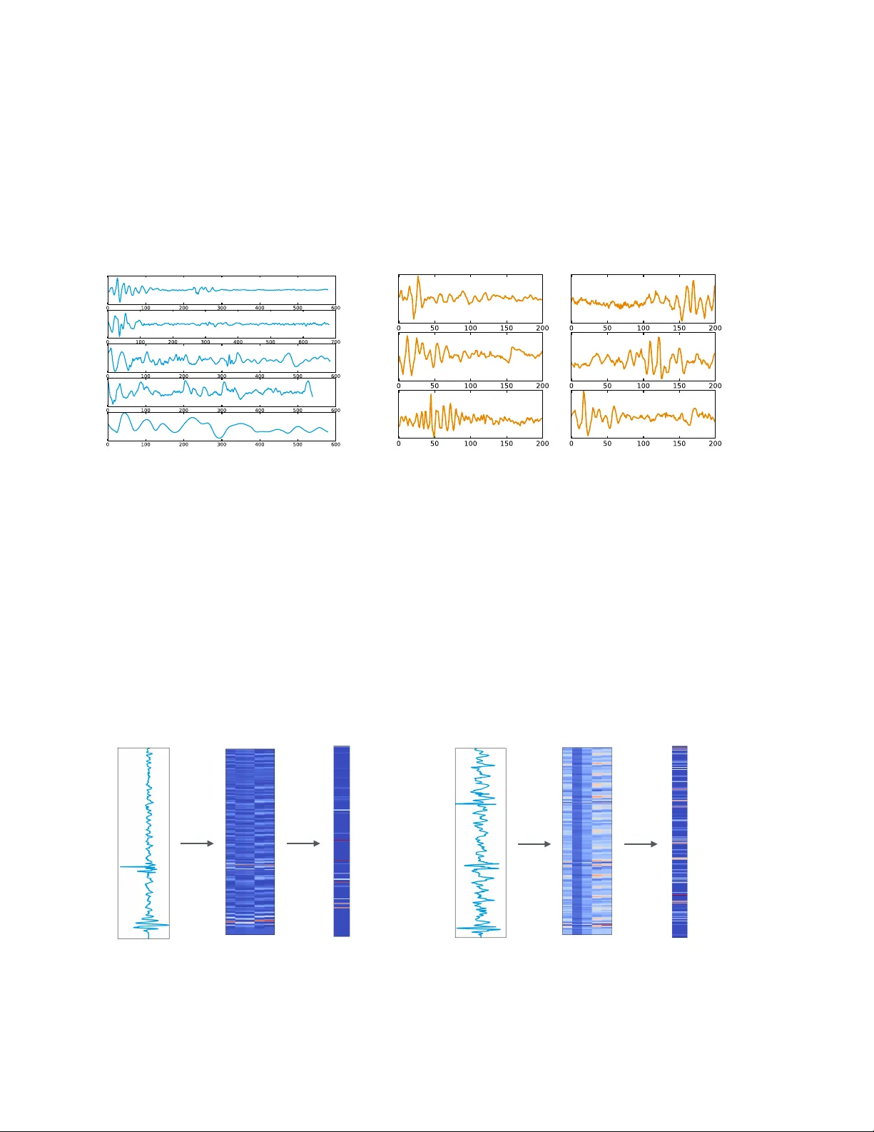
1 SEGMENT AL CONV OLUTIONAL NEURAL NETW ORKS F OR DETECTION OF CARDIA C ABNORMALITY WITH NOISY HEAR T SOUND RECORDINGS ∗ YUHA O ZHANG 1 , SANDEEP A YY AR 1 , LONG-HUEI CHEN 2 , ETHAN J. LI 2,3 1 Biome dic al Informatics T r aining Pr o gr am, Stanfor d University Scho ol of Me dicine 2 Dep artment of Computer Scienc e, 3 Dep artment of Bio engine ering, Stanfor d University Stanfor d, CA 94305, USA Email: yuhaozhang@stanfor d.e du, ayyars@stanfor d.e du, longhuei@stanfor d.e du, ethanli@stanfor d.e du Heart diseases constitute a global health burden, and the problem is exacerbated by the error-prone nature of listening to and interpreting heart sounds. This motiv ates the dev elopment of automated classification to screen for abnormal heart sounds. Existing machine learning-based systems ac hieve accurate classification of heart sound recordings but rely on exp ert features that hav e not b een thoroughly ev aluated on noisy recordings. Here w e propose a segmental conv olutional neural net- w ork architecture that ac hiev es automatic feature learning from noisy heart sound recordings. Our exp erimen ts show that our best model, trained on noisy recording segments acquired with an ex- isting hidden semi-marko v model-based approach, attains a classification accuracy of 87.5% on the 2016 Ph ysioNet/CinC Challenge dataset, compared to the 84.6% accuracy of the state-of-the-art statistical classifier trained and ev aluated on the same dataset. Our results indicate the p oten tial of using neural net work-based methods to increase the accuracy of automated classification of heart sound recordings for impro ved screening of heart diseases. 1. In tro duction Heart diseases constitute a significan t global health burden. Just one subset of these dis- eases, v alvular heart disease (VHD) resulting from rheumatic fev er, causes 300,000-500,000 prev en table deaths each year globally , primarily in developing countries. 1,2 Early detection of many heart diseases is crucial for optimal treatmen t managemen t to preven t disease pro- gression. 3,4 In dev eloping coun tries, the standard practice for screening of heart diseases suc h as VHD and cardiac arrh ythmia is cardiac auscultation to listen for abnormal heart sounds. P atien ts found to hav e suspicious abnormalities are then referred to sp ecialists for prop er diagnosis by a m uc h more expensive ec ho cardiographic pro cedure. 3 Although cardiac auscul- tation has b een replaced by ec ho cardiography for screening in industrialized countries, the cost-effectiv eness and pro cedural simplicity of auscultation mak e it an imp ortan t screening to ol for primary care pro viders and clinicians in under-resourced communities. 5,6 The main c hallenge in cardiac auscultation is the difficulty of detecting and interpreting subtle acoustic features asso ciated with heart sound abnormalities. Man ual classification of heart sounds suffers from high intra-observ er v ariabilit y, 7–14 causing false p ositive and false negativ e results. Muc h work has b een done in trying to impro v e screening accuracy , including efforts to design devices to record heart sounds and automatically classify them. Ho wev er, the biggest c hallenge for this task remains in dev eloping an accurate classifier for heart sound ∗ This w ork w as finished in Ma y 2016, and remains unpublished un til Decem b er 2016 due to a request from the data provider. 2 recordings, whic h are often obtained in noisy en vironmen ts. Here, w e propose a no vel approac h based on segmental conv olutional neural net w orks to classification of heart sound recordings. Our approach ac hieves automatic feature learning together with accurate prediction of the abnormalit y . On noisy recordings, this approac h outp erforms prior classifiers using a state-of- the-art feature set dev elop ed for noiseless recordings. The rest of this pap er is organized as follo ws. In Section 2, we discuss related previous researc h. In Section 3, w e introduce the metho ds that we used to classify noisy heart sound recordings, including prepro cessing of data, the use of traditional classifiers, and our segmen tal con v olutional neural net work models. Next, in Section 4, w e present the p erformance of our classifiers, along with our analysis of these results. W e discuss the limitations of our work and future directions in Section 5 and conclude our w ork in Section 6. 2. Related W ork The first step in automatic classification of heart sounds is segmentation of the recordings along heartbeat cycle b oundaries. Segmen tation divides the heart sound signal into cycles of four parts: the first heart sound (S1), systole, the second heart sound (S2), and diastole. P ast efforts in the field include the use of env elop e-based metho ds 15,16 and mac hine learning tec hniques. 17,18 A recen t segmentation algorithm proposed b y Schmidt et al has b een shown to work w ell on a large dataset of 10,172 heart sound recordings, and ac hieved an a verage of 95.63% F1 score, easily outstripping all other metho ds ev aluated with the same set of recordings in the literature. 19,20 This hidden semi-Mark ov mo del (HSMM)-based mo del was tested on noisy , real-world recordings and considered state-of-the-art. Therefore, we emplo y ed the algorithm as-is to acquire the segmen tation of input recordings. Previous work in heart sound recordings classification follows the traditional paradigm of using hand-crafted feature sets as input to automatic classification based on mac hine learning. F eatures are t ypically a mixture of time domain prop erties, frequency domain prop erties, statistical prop erties, and transform domain prop erties suc h as from the discrete w av elet transform (D WT) or empirical mo de decomp osition (EMD). 21 The extracted features are then fed to differen t mac hine learning metho ds, whic h are then trained to recognize abnormal heart sounds, or in some cases to classify the recordings in to the sp ecific heart diseases. The most common metho ds are artificial neural net w orks (ANNs), 22 supp ort v ector mac hines (SVMs), 23 Hidden Marko v mo dels (HMM), 24 and k-nearest neigh b ors (kNN). 25 Ho w ever, prior results ha v e b een restricted b y the use of small or otherwise limited data sets, including exclusion of noisy recordings or manual curation of recordings. While classifiers ha v e b een rep orted with accuracies ov er 90%, 26 there is insufficien t evidence to conclude whether the exp ert features used with these classifiers are fully applicable to noisy heart sound recordings. W e address this issue by training and testing traditional classifiers on a newly published set of noisy recordings. In addition, our work is inspired b y numerous recent work on the application of neural net w orks to the processing of sensory-t yp e data, such as visual 27–29 and sp eec h recognition. 30 Ho w ever, our segmental conv olutional neural netw ork approach is substan tially different from these work in its use of heart sound segments during training and test time. Meanwhile, w e also empirically ev aluated tw o differen t types of netw ork arc hitectures and tried to explain 3 their effectiveness via visualizations of learned filters and hidden la y ers. 3. Metho ds The heard sound recordings used in our exp erimen ts were obtained from a publicly hosted dataset 26 for the 2016 Ph ysioNet/Computing in Cardiology Challenge b . This dataset consists of approximately 3000 recordings obtained with a v ariety of durations, noise c haracteristics, and acoustic features. Cardiac conditions featured in the recordings include v alvular heart diseases, b enign murm urs, aortic disease, and arrh ythmias. Recordings in the dataset were collected from different lo cations on the bo dy of b oth c hildren and adults. Given the uncon- trolled en vironmen t, man y recordings are corrupted by v arious noise sources, such as talking, stethoscop e motion, breathing and intestinal sounds, whic h comprise the challenge of learning features and classifying the signals. As the dataset is in tended to supp ort the developmen t of classification systems for initial screening of heart diseases, recordings w ere only lab eled as normal or abnormal, dep ending on whether follow-up for further diagnosis w as recommended from the recording. At the time of our work, recordings excessiv ely corrupted by noise had not y et b een relabeled as unclassifiable b y c hallenge organizers, therefore our experiments w ere fo cused on binary classification b et w een normal and abnormal noisy recordings, whic h resp ectiv ely constituted 80% and 20% of the public dataset. W e split the dataset in to a 90% training set for classification model dev elopmen t and a 10% testing set for mo del ev aluation. In the absence of prior probabilities for disease prev alence, we constructed the test set to b e balanced b et w een normal and abnormal recordings for clearer in terpretabilit y of p erformance metrics. As a result, 17% of the recordings in the training set were abnormal and the remaining 83% w ere normal. W e preprocessed the recordings and then used them for tw o independent branc hes of inv estigation: traditional classification with feature selection, and the use of a new segmental con v olutional neural netw ork architecture. W e compared the test set p erformance of the results of these tw o in vestigations b y calculating sensitivit y , sp ecificit y , and accuracy , as these metrics are standard in prior w ork on heart sound classification. F or completeness, w e also compared area under the Receiver-Operating Characteristic (ROC) curv e and p ositive predictiv e v alue. 3.1. Pr epr o c essing As a first step, we prepro cess the recordings to handle noise and segment individual heart- b eats. As stated in the related w ork section, we employ a recen t HSMM-based segmen tation algorithm dev elop ed for noisy heard sound recordings, whic h has been rep orted to ac hiev e an accuracy of 95% on a b enchmark dataset. Since the signals were recorded from m ultiple sources and differ widely in levels of bac k- ground noise, w e iden tify the handling of noise within the data crucial for the success of do wnstream comp onen ts. W e explore a few common v en ues for denoising in the heart sound recordings and general signal pro cessing, including tec hniques based on discrete w av elet trans- form (DWT) 31 and empirical mo de decomp osition (EMD). In w av elet-based denoising, the b The data was obtained from the w ebsite: h ttps://physionet.org/c hallenge/2016/ 4 signal is reconstructed from thresholded comp onen ts pro duced with DWT using multi-lev el w a velet coefficients. This approach is finally used in our exp erimen ts, given its ease of imple- men tation. As the noise selection and reduction can v ary widely across the m ultiple data sources and individual cases, we also in tegrate the denoising results as a feature in traditional classification metho ds by calculating the signal-to-noise (SNR) of the individual recordings. 3.2. T r aditional Machine L e arning-b ase d Classifiers W e inv estigated the p erformance of v arious machine learning-based classifiers with hand- designed features on noisy heart sound recordings. Through this inv estigation, we would lik e to understand: 1) the con tribution of differen t hand-designed features for the classification of noisy heart records; and 2) the ov erall p erformance of traditional approaches on this new dataset. 3.2.1. F e atur es W e attempt to implemen t features from a published study for classifying minimal-noise record- ings as either normal or abnormal with extraction of 23 features and subsequent selection of 5 features. 32 P er recording, w e extract a set of 58 time-domain, frequency-domain, and transform-domain features which together constituted a sup erset of the 23 published features, as shown in T able 1. All features are represented by the mean and standard deviation ov er all heart b eat cycles in the recording. T o ac hiev e b etter results, w e transform and com bine some features as ratios. Some frequency domain features hav e missing v alues due to anomalous recording conten t. T able 1. F eatures extracted for traditional classification. Ov erall F eature Type F eature Type Num b er of F eatures Time Domain In terv al Length 16 Absolute Amplitude 5 T otal Po w er 5 Zero Crossing Rate 1 Amplitude at Peak F requency 5 F requency Domain P eak F requency 5 Bandwidth 9 Q-F actor 9 T otal Harmonic Distortion 1 T ransform Domain Cepstrum Peak Amplitude 1 Signal-to-Noise Ratio from D WT 1 3.2.2. Mo dels W e emplo y differen t statistical mo dels to p erform sup ervised learning from the dataset. Before training, w e impute all the missing data using median v alues across all training examples. W e p erform 10-fold cross v alidation to ev aluate mo del p erformance on our 90% im balanced 5 training data set. T o alleviate classifier bias in learning one class ov er the other, we follo w the standard procedure to increase the w eigh ts of classification errors of abnormal recordings. W e also use 10-fold cross v alidation for tuning classifier hyperparameters to improv e mo del p erformance. Our mo dels and corresp onding hyperparameters are sho wn in T able 2. T able 2. Hyperparameters tuned for the inv estigated classification mo dels. Classification Mo del T uning Parameters Logistic Regression - Lasso, Ridge Based Metho ds regularizing/p enalizing term Supp ort V ector Machine k ernel function, cost, gamma Decision T rees n umber of trees Random F orests n umber of estimators, num ber of features K-Nearest Neighbours n umber of neighbours W e use forw ard step wise, backw ard step wise, and Lasso regression metho ds for feature selection. W e use features selected b y the forw ard step wise and Lasso metho ds for training the logistic regression classifier and Lasso-selected features for training the remaining classifiers. F or the Lasso metho d, we optimize the regularization/tuning parameter lam b da and select features using the lam b da v alue that minimizes the misclassification error rate. 3.3. Se gmental Convolutional Neur al Networks for He art Sound Classific ation T raditional classifiers are simple to emplo y and fast to train, but rely on hand-designed features that do not necessarily capture useful signals in the recordings. An alternative to traditional classifiers is mo dels that can automatically learn useful features that are not limited b y h uman design. Among these mo dels, conv olutional neural netw ork (CNN) provides a flexible filter- based architecture to capture the patterns in the sensory-t yp e data. How ever, heart sound signals v ary in length significantly , and often con tain noise that mak es a certain snipp et of signal unclassifiable. These mak e the adoption of CNN mo dels less straigh tforw ard. … Input Signal CNN Unit T raining T ime T est Time … 1 0 1 … 0 / 1 Fig. 1. T raining and ev aluation of the segmental conv olutional neural netw orks. W e propose a segmen tal con v olutional neural net work arc hitecture to solv e these problems. 6 As sho wn in Fig. 1, our metho d tak es ra w heart sound recordings as input, and acquires recording segments b y using the hidden semi-marko v mo del describ ed in Section 3.1. Then we only k eep segments with lengths from 400 to 1200 and zero-pad all signals into a 1200-elemen t v ector. During training time, this prepro cessing step keeps 98% of all segments and lea ves us with 76509 training segments. W e then cast these training segmen ts as a new training set to train our CNN units. During test time, we first split eac h test signal into segments and then classify each segment using our trained CNN unit. Then w e com bine the segment classifications and classify a recording as abnormal only when the prop ortion of segments classified as abnormal is o v er a threshold. W e treat this threshold v alue as a h yp erparameter. This approac h has three k ey adv an tages. First, since standard CNN requires fixed-length input, this naturally solv es the input length normalization issue. Second, expanding signals in to segments substan tially increases the num b er of training instances, which has b een prov ed to b e critical in the success of other applications of neural net works. Third, global classification of a recording is more robust against accidental noise in the data, as accidental noise can only influence the classification of a small portion of lo cal segments. Filter configuration and depth are tw o ma jor factors that influence the p erformance of a CNN mo del. It remains unclear which t yp e of architecture is more suitable to this task. Therefore, w e no w discuss the use of t w o differen t architectures for CNN units, whic h w e name Filter-fo cused CNNs and Depth-fo cused CNNs resp ectively . These t w o architecture t yp es differ mainly in their configuration of filters, the w a y max-p o oling is conducted, and the w ay differen t lay ers are stac ked. 3.3.1. Filter-fo cuse d CNN (FCNN) Heart Sound Recording V ector Representation Feature Maps Hidden Representation Output Probabilities Discretization Convolution Max-pooling Fully-connected + Softmax Fig. 2. Architecture of a FCNN mo del. Fig. 2 visualizes the architecture of a FCNN mo del. In a F CNN mo del, a heart sound segmen t will first b e represen ted as a v ector x , with eac h element in x represen ting the nor- malized amplitude of the signal at that time p oin t. The core parameters of the net w ork are a set of filters with differen t windo w sizes that will b e applied to the input signal x . Giv en a sp ecific window size w , a filter is a v ector of size w f = [ f 1 , f 2 , ..., f w ] , where each f i is a scalar. 7 A feature map m of this filter can b e obtained from the application of a 1D-con v olutional op erator on f and x to pro duce an output sequence m = [ m 1 , m 2 , ..., m n − w +1 ] where n is the length of input signal x : m i = g ( w − 1 X j =0 f j +1 x j + i + b ) where b is a bias term and g is a non-linear function. This con v olution pro cess is repeated for man y filters of differen t windo w sizes w . After the con v olution lay er, a max-o ver-time p o oling op eration is applied to eac h feature map m k to generate a single scalar activ ation h k : h k = max([ m k 1 , m k 2 , ..., m k n − w +1 ]) And then all activ ations h k are concatenated to form a size- N hidden representation of the original signal h = [ h 1 , h 2 , ..., h N ] . The idea b ehind the max-ov er-time p o oling op eration is to only k eep the most ob vious activ ation that are generated b y the con v olution, and use that to c haracterize the signal for the downstream classification. Finally , the hidden represen tation h is fed in to a fully-connected with softmax lay er to generate the class probabilities y . W e use cross entrop y b et w een predicted lab els and ground truth lab els as loss function. The in tuition b ehind the use of man y filters of v arious windo w sizes is that the mo del should b e able to learn through bac k-propagation common patterns that it has seen in the training signals that are useful for the classification, and these patterns could p otentially b e n umerous and of differen t scales. 3.3.2. Depth-fo cuse d CNN (DCNN) Heart Sound Recording V ector Representation Final Representation Output Pro b a b i l i t i e s Discretization Convolution Max-pooling Softmax ….. Condensed Representation Repeated Layers Hidden Representation Fully-connected Fig. 3. Architecture of a DCNN mo del. While large filters of v arious sizes can help to capture useful patterns of different scales, it ma y also b e useful to hav e a model with only small filters at eac h lay er but focuses on stac king man y lay ers together to form a deep arc hitecture, as has b een found in visual recognition tasks. 28 Fig. 3 visualizes the architecture of a Depth-fo cused CNN mo del. There are three ma jor differences b etw een DCNNs and FCNNs. First, the filter sizes in DCNNs are muc h 8 smaller than in F CNNs. Typically , the size of DCNN filters are appro ximately 10, while the size of FCNN filters can range from 10 to 500. The use of very small filters in DCNNs reduces the computational cost to p erform con volutional op erations and thus enables us to explore deep er mo dels while still capturing useful patterns in the signals. Second, in DCNNs, the motif of a con v olution lay er follo w ed by a max-p o oling lay er is rep eated several times to form a hidden representation of the original signal. Then this hidden represen tation is fed in to multiple stack ed fully-connected la y ers to reduce the represen tation size, after whic h the softmax lay er generates the output probabilities. Finally , the wa y con volution and max p o oling are conducted is different. In a DCNN con v olution lay er, the output of conv olution op eration is a feature matrix m = [ m 1 , m 2 , ..., m n ] , where eac h column m i is the feature map vector obtained from filter f i con v olved with signal x , and can b e view ed as a “channel” in the output signal. Then at the po oling la y er, instead of doing a max-o v er-time p o oling, a max po oling ov er the local time region is p erformed, and c hannels are k ept. F or example, a max-p o oling op eration with windo w 2 is: ˆ m c i = max( m c 2 i , m c 2 i +1 ) where ˆ m c represen ts the p o oling output column in c hannel c , and m c represen ts the channel c column in the feature matrix. Here, the max p o oling serv es as a sub-sampling ov er the signal and preserves more information compared to the max-o ver-time p o oling operation in F CNN. 3.3.3. Network Configur ations W e design exp erimen ts to ev aluate our segmen tal conv olutional neural net work approac h. T able 3 shows the CNN arc hitectures that we rep ort results on. W e explored a lot different arc hitectures and included results for these mo dels b ecause: First, these mo dels demonstrate progressiv ely increasing filter sizes and net w ork depths, enabling comparison of the effects of different net w ork configurations on final p erformance; Second, the training times of these mo dels are tolerable giv en the resources w e ha ve. In the table, “Con v” represen ts a con volution la y er, “MP” a max-p o oling la y er, and “FC” a fully-connected lay er. F or instance, for FCNNs, “Con v([50-500,50]*20)” represents a con v olution lay er with windo w size ranging from 50 to 500 with a step of 50, and eac h window size corresp onds to 20 different filters. F or DCNNs, “Con v([10*25])” represents a con volution lay er with 25 filters and window size 10. T able 3. CNN netw ork configurations. CNN Mo del Arc hitecture Configuration # Lay ers # Filters F CNN-Small Con v([50-500,50]*20), MP , FC 3 200 F CNN-Medium Con v([25-500,25]*30), MP , FC 3 600 F CNN-Large Con v([20-600, 20]*50), MP , F C 3 1500 DCNN-Shallo w Con v([10]*25), MP , Conv([10]*50), MP , FC(256), F C 6 75 DCNN-Deep Con v([10]*25), MP , Conv([10]*50), MP , Conv([10]*50), MP , FC(256), FC 8 125 F or all CNN configurations, w e use L2 regularization on the weigh ts and drop out 33 b efore the last softmax la y er to regularize the mo del. W e use AdaGrad 34 to train the mo dels with error bac kpropagation. W e train each mo del on a 90% subset of our training set for 50 ep o c hs, and 9 after eac h epo ch we ev aluate the mo del on the remaining 10% v alidation subset of our training set. F or each CNN configuration, we sav e the model that generates the b est accuracy on the v alidation set as the final mo del. This allows us to preven t the final mo del from ov erfitting on the training data. W e then ev aluate the b est mo del from each CNN configuration on the same test set as used by the traditional classifiers. 4. Results 4.1. T r aditional Classifiers T able 4 compares the p erformance of the traditional classification mo dels. W e ev aluated mo del p erformance based on accuracy , sp ecificit y , sensitivit y , p ositiv e predictive v alue (PPV), and area under the receiver op erating characteristic curve (A UC). The receiver op erating c har- acteristic (ROC) curves for all mo dels are shown in Fig. 4. W eigh ting and feature selection significan tly improv ed p erformance of most metho ds except decision trees. Ov erall, we saw that SVM with feature selection was the b est p erforming mo del. How ev er, the accuracy of this mo del on noisy recordings w as lo w er than the published accuracies of mo dels using the same feature set on lo w-noise recordings, whic h exceeded 90% with feature selection. 32 T able 5 summarizes the features selected by our mo dels. Con trasting with the previous w ork which found that four time-domain features and one frequency-domain feature w ere suffi- cien t for accurate classification of low-noise recordings, 32 w e found that accurate classification of noisy recordings required additional frequency-domain and transform-domain features. T able 4. Results for different traditional classification mo dels on the test set. The num bers in parentheses show the baseline p erformances of the mo dels, whereas those outside show p er- formances after mo del impro vemen t, namely weigh ting, parameter tuning, and feature selection. Classifier Accuracy (%) Sp ecificity (%) Sensitivit y (%) PPV (%) A UC (%) SVM 84.6 (69.2) 92.2 (68.3) 78.3 (56.2) 89.2 (63.4) 83.4 (55.4) Logistic Regression 75.4 (49.5) 74.3 (62.4) 75.1 (50.2) 74.3 (55.4) 81.3 (65.4) Random F orests 71.4 (65.4) 91.3 (68.2) 72.3 (65.4) 81.3 (71.3) 88.4 (71.4) KNN (k=3) 60.3 (56.1) 92.2 (65.3) 60.7 (57.6) 82.4 (79.4) 71.3 (65.4) Naiv e Ba yes 70.4 (53.4) 60.3 (56.7) 71.5 (53.3) 71.5 (60.6) 77.7 (62.3) Decision T rees 73.3 (73.6) 88.4 (88.6) 73.4 (73.6) 85.5 (85.5) 69.4 (58.6) T able 5. F eature selection results. F eature Type Num b er of F eatures Time Domain 5 F requency Domain 6 T ransform Domain 2 4.2. Se gmental Convolutional Neur al Networks T able 6 shows the results of differen t segmental con v olutional neural net w ork mo dels on the test set, with the mo del names corresp onding to configurations in T able 3. Overall, our DCNN- 10 Fig. 4. ROC curv es for classification mo dels. Deep model produces the best accuracy , specificity and PPV results, while our DCNN-Shallow mo del pro duces the b est sensitivit y . F or F CNN mo dels, as filter n umber increases, we observed an increase in all metrics except sensitivit y . This suggests that, in F CNN mo dels, a larger n um b er of filters with more fine-grained windo w sizes can help the mo del capture more patterns in the signals, which aligns well with our in tuitions. It is w orth noting that the F CNN-Large mo del already pro duced a relativ ely high accuracy , and the highest sensitivity v alue. F or DCNN mo dels, as the num b er of la yers increases, w e observe increases in almost all metrics (except sensitivit y), which suggests that deep er mo dels with more lay ers can help the model learn b etter patterns in the signals, which aligns with our assumptions. In addition, compared to F CNN mo dels, w e observed that DCNN mo dels almost alw a ys p erform b etter, whic h suggests that a deep mo del with small filter sizes and few filters at eac h lay er is more expressiv e in mo deling the heart sound signal data than a shallow model with a large n umber of filters. How ever, in terms of sensitivity , we also disco v ered that the p erformance do es not change m uc h as the filter num ber and lay er num ber increase. In other w ords, most of the gain in accuracy comes from the gain in sp ecificity . T able 6. Classification results for different CNN configurations, with SVM for comparison. CNN Mo del Accuracy (%) Sp ecificity (%) Sensitivit y (%) PPV (%) F CNN-Small 81.2 72.9 89.2 77.0 F CNN-Medium 83.4 78.1 88.6 80.5 F CNN-Large 85.3 80.0 90.5 82.2 DCNN-Shallo w 86.9 83.2 90.5 84.6 DCNN-Deep 87.5 88.4 86.7 88.4 SVM 84.6 92.2 78.3 89.2 4.3. CNN Visualizations T o understand how the segmen tal con volutional neural netw orks w ork, w e plot visualizations of randomly selected heart sound segments in the training dataset and filters learned b y the FCNN-Small mo del in Fig. 5. The input segments hav e v ery different shap es, and noise is 11 observ able in some segmen ts. This suggests the difficult y of the classification task. In addition, the visualization of filters shows that the net w ork learned very go o d wa v eform-lik e patterns from the training data. This is ev en more convincing, considering the fact that all filters w ere randomly initialized prior to training. This qualitative result aligns very well with our in tuitions ab out why CNN mo dels are suitable for heart sound classification. (a) (b) Fig. 5. (a) Visualization of randomly c hosen segmen ts in the training data; (b) Visualization of learned filters (windo w size 200) by F CNN-Small mo del. Fig. 6 shows the netw ork activ ations for normal and abnormal input segments. W e find that, giv en the input segmen t, some of the output neurons in conv olution lay ers activ ate, whic h indicates a pattern matched strongly with the signal at that lo cal region, while others do not activ ate. Moreo v er, w e find that more neurons in b oth the con v olution la y ers and hidden la y er are activ ated by abnormal segmen ts compared to normal segmen ts, indicating that many learned filters in the net w ork are patterns of abnormal signals. conv1 activations final representation input segment (a) conv1 activations final representation input segment (b) Fig. 6. Visualization of netw ork activ ations for (a) a normal heart sound segment and (b) an abnormal segmen t. All activ ations are from DCNN-Deep mo del, and only activ ations in the first con v olution lay er and the final hidden la yer are shown. Red color represents an activ ation v alue of 1, while blue color represents an activ ation v alue of 0. 12 4.4. Comp arison W e compared the p erformance of the best p erforming CNN architectures, namely DCNN- Large and F CNN-Deep, to SVM, which was the b est p erforming model among the traditional classifiers (T able 6). W e see that CNNs outp erform SVM significan tly for accuracy and sen- sitivit y . While F CNN-Deep has marginally b etter sp ecificity , DCNN-Large has b etter p erfor- mance in terms of accuracy and sensitivity . Our results show that application of CNNs to noisy heart sound recordings can pro duce b etter classification as compared to applying tra- ditional classification tec hniques. Due to time limits, we were not able to fully explore the arc hitecture space of the CNN mo dels. Therefore, we believe that our segmen tal con v olutional neural netw ork approac h has even more p otential in classifying heart sound recordings than w e hav e found. 5. Discussion Our inv estigation of the applicabilit y of previously published w ork in traditional classification to noisy heart sound recordings suggests that further ev aluation is needed. W e found significant differences from feature extraction and classifier performance results rep orted from one such study , which justifies more rigorous scrutiny of previous w ork. Sp ecifically , it would b e useful to v erify that feature extraction and traditional classification do es indeed p erform b etter on a dataset of clean heart sound recordings. Due to limits of computing resources, we hav e not y et fully realized the p otential of our CNN mo dels. W e b eliev e that b etter-p erforming models with more filters and more lay ers can b e ac hieved by doing a more thorough h yp erparameter search. Another clear av en ue of exploration is to decomp ose the signals further with EMD, which has b een shown to delineate signals and noises of differen t origins in heart sound recordings. 20 W e would lik e to examine ho w splitting a recording into EMD comp onen ts for use as separate input c hannels to our segmen tal CNNs ma y increase classification accuracy . Limited by the annotation in the training data, our work is fo cused on the binary clas- sification of heart sound recordings into normal and abnormal categories. Ho w ev er, it is also practically useful to predict a third “unclassifiable” category , esp ecially when noise is domi- nan t in the heard sound recordings. F or example, in real w orld applications, this third lab el can serve as a signal for human in terven tion. Therefore another direction for future w ork is to explore the com bination of sup ervised and unsup ervised approaches to pro duce this “unclas- sifiable” lab el accurately . 6. Conclusion W e prop ose a segmental conv olutional neural netw ork approac h to accurately classify noisy heart sound recordings. W e studies the effectiv eness of tw o differen t types of conv olutional neural net work arc hitectures, and compare their results with the application of traditional statistical classifiers on a set of manually curated features. Our results suggest that: First, traditional statistical classifiers using feature sets developed for lo w-noise recordings may p erform w orse on noisy recordings. Second, segmen tal conv olutional neural netw orks with 13 deep arc hitectures and small filters can achiev e higher accuracy in classifying noisy heart sound recordings without relying on manually-curated feature sets. 7. Ac kno wledgemen ts The authors w ould like to ackno wledge Dr. Russ Altman, Dr. Steven Bagley and Dr. David Stark at Stanford Universit y for their helpful suggestions to improv e this work. W e also wan t to thank Dr. Victor F ro elicher for a helpful discussion on v alvular heart diseases. References 1. W. H. O. E. Consultation, Rheumatic F ever and Rheumatic He art Dise ase , tech. rep., W orld Health Organization (2001). 2. J. R. Carapetis, Cir culation 118 , 2748 (2008). 3. E. Marijon, P . Ou, D. S. Celerma jer, B. F erreira, A. O. Mo cum bi, D. Sidi and X. Jouven, Bul letin of the World He alth Or ganization 86 , 84 (2008). 4. B. J. Gersh, Auscultation of cardiac m urmurs in adults. In: UpT oDate, (2015). 5. J. M. Szta jzel, M. Picard-Kossovsky , R. Lerch, C. V uille and F. P . Sarasin, International journal of c ar diolo gy 138 , 308 (2010). 6. I. Maglogiannis, E. Loukis, E. Zafirop oulos and A. Stasis, Computer metho ds and pr o gr ams in biome dicine 95 , 47 (2009). 7. C. E. Lok, C. D. Morgan and N. Ranganathan, CHEST Journal 114 , 1283 (1998). 8. A. A. Ishmail, S. Wing, J. F erguson, T. A. Hutchinson, S. Magder and K. M. Flegel, CHEST Journal 91 , 870 (1987). 9. M. D. Jordan, C. R. T a ylor, A. W. Nyh uis and M. E. T a vel, Ar chives of internal me dicine 147 , 721 (1987). 10. J. M. V uk anovic-Criley , S. Criley , C. M. W arde, J. R. Boker, L. Guev ara-Matheus, W. H. Ch urchill, W. P . Nelson and J. M. Criley , Ar chives of internal me dicine 166 , 610 (2006). 11. S. K. March, J. L. Bedynek and M. A. Chizner, T eaching cardiac ausc ultation: effectiveness of a patien t-cen tered teac hing conference on improving cardiac auscultatory skills, in Mayo Clinic Pr o c e e dings , (11)2005. 12. J. M. V uk anovic-Criley , A. Ho v anesyan, S. R. Criley , T. J. Ryan, G. Plotnick, K. Mank owitz, C. R. Conti and J. M. Criley , Clinic al c ar diolo gy 33 , 738 (2010). 13. S. Mangione and L. Z. Nieman, Jama 278 , 717 (1997). 14. M. E. T av el, Cir culation 93 , 1250 (1996). 15. H. Liang, S. Lukk arinen and I. Hartimo, Heart sound segmen tation algorithm based on heart sound env elogram, in Computers in Car diolo gy 1997 , 1997. 16. S. Sun, Z. Jiang, H. W ang and Y. F ang, Computer metho ds and pr o gr ams in biome dicine 114 , 219 (2014). 17. T. Oskip er and R. W atrous, Detection of the first heart sound using a time-dela y neural net w ork, in Computers in Car diolo gy, 2002 , 2002. 18. T. Chen, K. Kuan, L. A. Celi and G. D. Clifford, Intelligen t heartsound diagnostics on a cellphone using a hands-free kit., in AAAI Spring Symp osium: Artificial Intel ligenc e for Development , 2010. 19. S. Schmidt, C. Holst-Hansen, C. Graff, E. T oft and J. J. Struijk, Physiolo gic al Me asur ement 31 , p. 513 (2010). 20. C. D. P apadaniil and L. J. Hadjileontiadis, IEEE journal of biome dic al and he alth informatics 18 , 1138 (2014). 21. S. Leng, R. San T an, K. T. C. Chai, C. W ang, D. Ghista and L. Zhong, Biome dic al engine ering online 14 , p. 1 (2015). 14 22. H. U˘ guz, Journal of me dic al systems 36 , 61 (2012). 23. A. Ghareh baghi, I. Ekman, P . Ask, E. Nylander and B. Janerot-Sjoberg, International journal of c ar diolo gy 198 , p. 58 (2015). 24. R. Sara¸ cO˘ gLu, Engine ering Applic ations of Artificial Intel ligenc e 25 , 1523 (2012). 25. L. Av endano-V alencia, J. Go dino-Lloren te, M. Blanco-V elasco and G. Castellanos-Dominguez, A nnals of Biome dic al Engine ering 38 , 2716 (2010). 26. C. Liu, D. Springer, Q. Li, B. Mo o dy , R. A. Juan, F. J. Chorro, F. Castells, J. M. Roig, I. Silv a, A. E. Johnson et al. , Physiolo gic al Me asur ement 37 , p. 2181 (2016). 27. A. Krizhevsky , I. Sutskev er and G. E. Hin ton, Imagenet classification with deep conv olutional neural netw orks, in A dvanc es in neur al information pr o c essing systems , 2012. 28. K. Simon yan and A. Zisserman, arXiv pr eprint arXiv:1409.1556 (2014). 29. T. W ang, D. J. W u, A. Coates and A. Y. Ng, End-to-end text recognition with con v olutional neural netw orks, in Pattern R e c o gnition (ICPR), 2012 21st International Confer enc e on , 2012. 30. Y. LeCun and Y. Bengio, The handb o ok of br ain the ory and neur al networks 3361 , p. 1995 (1995). 31. D. Gradolewski and G. Redlarski, Computers in biolo gy and me dicine 52 , 119 (2014). 32. M. Singh and A. Cheema, International Journal of Computer Applic ations 77 (2013). 33. N. Sriv astav a, G. Hinton, A. Krizhevsky , I. Sutskev er and R. Salakhutdino v, The Journal of Machine L e arning R ese ar ch 15 , 1929 (2014). 34. J. Duc hi, E. Hazan and Y. Singer, The Journal of Machine L e arning R ese ar ch 12 , 2121 (2011).