Semi-Supervised Learning with the Deep Rendering Mixture Model

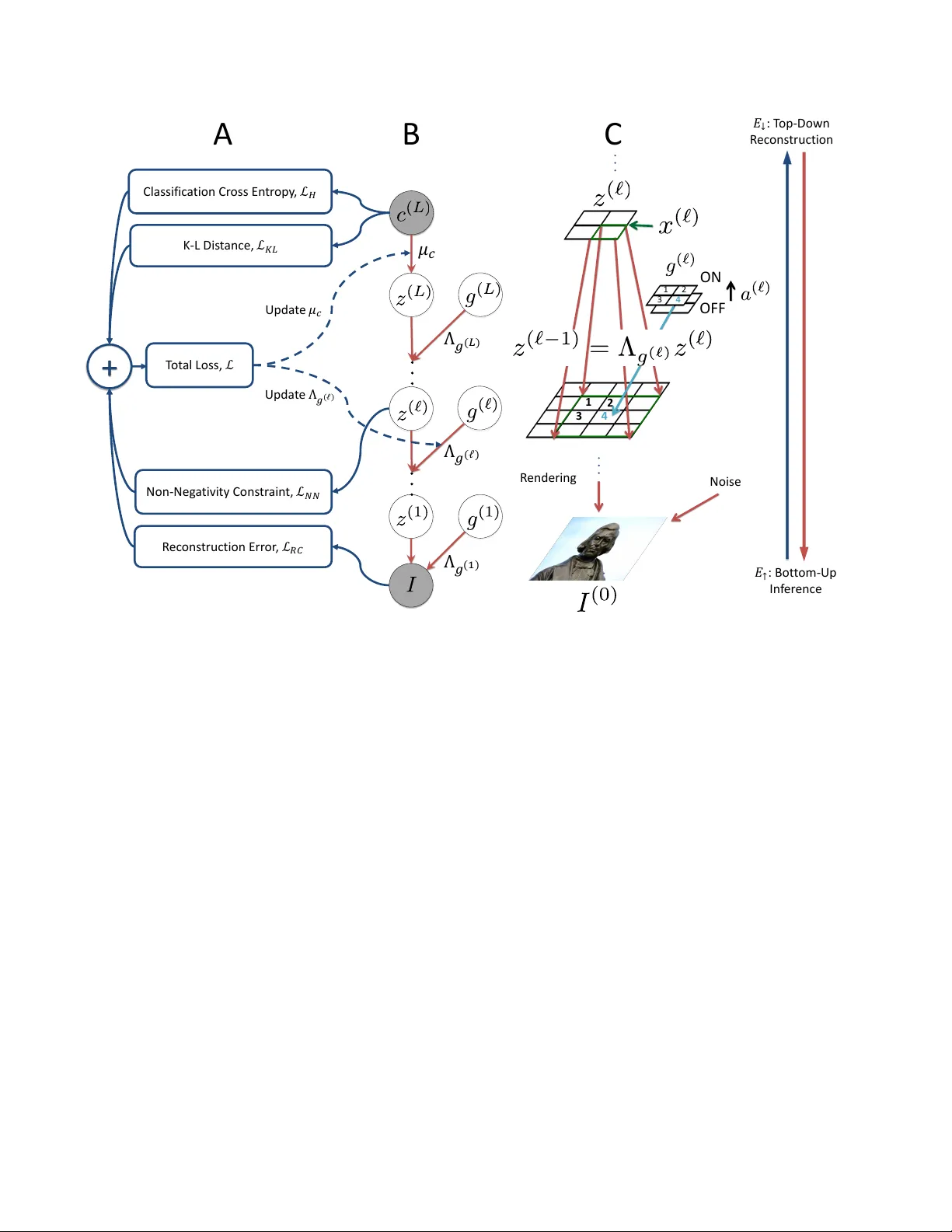
Semi-Supervised Lear ning with the Deep Rendering Mixtur e Model T an Nguyen 1 , 2 W anjia Liu 1 Ethan Perez 1 Richard G. Baraniuk 1 Ankit B. Patel 1 , 2 1 Rice Uni versity 2 Baylor College of Medicine 6100 Main Street, Houston, TX 77005 1 Baylor Plaza, Houston, TX 77030 {mn15, wl22, ethanperez, richb}@rice.edu ankitp@bcm.edu Abstract Semi-supervised learning algorithms r educe the high cost of acquiring labeled training data by using both la- beled and unlabeled data during learning. Deep Convo- lutional Networks (DCNs) have achie ved great success in supervised tasks and as such have been widely employed in the semi-supervised learning. In this paper we lever - age the recently developed Deep Rendering Mixtur e Model (DRMM), a pr obabilistic generative model that models la- tent nuisance variation, and whose infer ence algorithm yields DCNs. W e develop an EM algorithm for the DRMM to learn fr om both labeled and unlabeled data. Guided by the theory of the DRMM, we intr oduce a novel non- ne gativity constraint and a variational infer ence term. W e r eport state-of-the-art performance on MNIST and SVHN and competitive results on CIF AR10. W e also pr obe deeper into how a DRMM trained in a semi-supervised setting r ep- r esents latent nuisance variation using synthetically ren- der ed images. T aken together , our work pr ovides a uni- fied fr amework for supervised, unsupervised, and semi- supervised learning. 1. Introduction Humans are able to learn from both labeled and unla- beled data. Y oung infants can acquire kno wledge about the world and distinguish objects of dif ferent classes with only a fe w provided “labels”. Mathematically , this poverty of in- put implies that the data distrib ution p ( I ) contains informa- tion useful for inferring the category posterior p ( c | I ) . The ability to e xtract this useful hidden knowledge from the data in order to lev erage both labeled and unlabeled examples for inference and learning, i.e. semi-supervised learning, has been a long-sought after objectiv e in computer vision, machine learning and computational neuroscience. In the last fe w years, Deep Con v olutional Networks (DCNs) have emerged as powerful supervised learning models that achiev e near-human or super-human perfor- mance in various visual inference tasks, such as object recognition and image segmentation. Howe ver , DCNs are still far behind humans in semi-supervised learning tasks, in which only a fe w labels are av ailable. The main dif- ficulty in semi-supervised learning in DCNs is that, until recently , there has not been a mathematical framework for deep learning architectures. As a result, it is not clear ho w DCNs encode the data distribution, making combining su- pervised and unsupervised learning challenging. Recently , the Deep Rendering Mixture Model (DRMM) [ 13 , 14 ] has been developed as a probabilistic graphical model underlying DCNs. The DRMM is a hierarchical gen- erativ e model in which the image is rendered via multiple lev els of abstraction. It has been shown that the bottom- up inference in the DRMM corresponds to the feedforward propagation in the DCNs. The DRMM enables us to per - form semi-supervised learning with DCNs. Some prelimi- nary results for semi-supervised learning with the DRMM are provided in [ 14 ]. Those results are promising, but more work is needed to e valuate the algorithms across many tasks. In this paper , we systematically de velop a semi- supervised learning algorithm for the Non-negati ve DRMM (NN-DRMM), a DRMM in which the intermediate ren- dered templates are non-negati ve. Our algorithm contains a bottom-up inference pass to infer the nuisance variables in the data and a top-do wn pass that performs reconstruction. W e also employ v ariational inference and the non-negati ve nature of the NN-DRMM to derive two ne w penalty terms for the training objecti ve function. An overvie w of our al- gorithm is giv en in Figure 1 . W e v alidate our methods by showing state-of-the-art semi-supervised learning results on MNIST and SVHN, as well as comparable results to other state-of-the-art methods on CIF AR10. Finally , we analyze the trained model using a synthetically rendered dataset, which mimics CIF AR10 but has ground-truth labels for nui- sance variables, including the orientation and location of the object in the image. W e sho w ho w the trained NN-DRMM encodes nusiance variations across its layers and sho w a comparison against traditional DCNs. 1 1 2 3 4 1 2 4 3 R endering Noise ON OFF B C   : Bot t om - Up In f er ence   : T op - Down R ec ons truction Classific a tion Cr oss E n tr op y ,   K - L D is t ance,   Non - Neg a tivi ty Co ns tr ain t,   R ec ons truction Err or ,   T ot al Loss,  Upda t e   Upda t e   󰇛  󰇜     󰇛  󰇜   󰇛  󰇜   󰇛  󰇜 A Figure 1: Semi-supervised learning for Deep Rendering Mixture Model (DRMM) (A) Computation flow for semi-supervised DRMM loss function and its components. Dashed arrows indicate parameter update. (B) The Deep Rendering Mixture Model (DRMM). All dependence on pixel location x has been suppressed for clarity . (C) DRMM generativ e model: a single super pixel x ( ` ) at lev el ` (green, upper) renders down to a 3 × 3 image patch at lev el ` − 1 (green, lower), whose location is specified by g ( ` ) (light blue). (C) shows only the transformation from lev el ` of the hierarchy of abstraction to lev el ` − 1 . 2. Related W ork W e focus our revie w on semi-supervised methods that employ neural network structures and di vide them into dif- ferent types. A utoencoder-based Ar chitectures: Many early works in semi-supevised learning for neural networks are built upon autoencoders [ 1 ]. In autoencoders, the images are first projected onto a low-dimensional manifold via an encoding neural network and then reconstructed using a decoding neural network. The model is learned by minimizing the reconstruction error . This method is able to learn from unlabeled data and can be combined with traditional neural networks to perform semi-supervised learning. In this line of work are the Contractiv e Autoencoder [ 16 ], the Manifold T angent Classifier , the Pseudo-label Denoising Auto Encoder [ 9 ], the Winner -T ake-All Autoencoders [ 11 ], and the Stacked What-Where Autoencoder [ 20 ]. These architectures perform well when there are enough labels in the dataset but fail when the number of labels is reduced since the data distribution is not taken into account. Recently , the Ladder Network [ 15 ] was de veloped to overcome this shortcoming. The Ladder Network approximates a deep factor analyzer where each layer in the model is a factor analyzer . Deep neural networks are then used to do approximate bottom-up and top-down inference. Deep Generativ e Models: Another line of work in semi- supervised learning is to use neural networks to estimate the parameters of a probabilistic graphical model. This approach is applied when the inference in the graphical model is hard to derive or when the exact inference is computationally intractable. The Deep Generative Model family is in this line of work [ 7 , 10 ]. Both Ladder Networks and Deep Generativ e Models yield good semi-supervised learning performance on benchmarks. They are complementary to our semi- supervised learning on DRMM. Howe ver , our method is different from these approaches in that the DRMM is the graphical model underlying DCNs, and we theoretically deriv e our semi-supervised learning algorithm as a proper probabilistic inference against this graphical model. Generative Adversarial Networks (GANs): In the last few years a variety of GANs have achie ved promising re- sults in semi-supervised learning on different benchmarks, including MNIST , SVHN and CIF AR10. These models also generate good-looking images of natural objects. In GANs, two neural networks play a minimax game. One gener - ates images, and the other classifies images. The objectiv e function is the game’ s Nash equilibrium, which is dif ferent from standard object functions in probabilistic modeling. It would be both exciting and promising to extend the DRMM objectiv e to a minimax game as in GANs, but we lea ve this for future work. 3. Deep Rendering Mixture Model The Deep Rendering Mixture Model (DRMM) is a recently developed probabilistic generati ve model whose bottom-up inference, under a non-neg ativity assumption, is equiv alent to the feedforward propagation in a DCN [ 13 , 14 ]. It has been shown that the inference process in the DRMM is efficient due to the hierarchical structure of the model. In particular , the latent v ariations in the data are captured across multiple le vels in the DRMM. This factor- ized structure results in an exponential reduction of the free parameters in the model and enables efficient learning and inference. The DRMM can potentially be used for semi- supervised learning tasks [ 13 ]. Definition 1 ( Deep Rendering Mixture Model ) . The Deep Rendering Mixtur e Model (DRMM) is a deep Gaussian Mix- ture Model (GMM) with special constraints on the latent variables. Generation in the DRMM takes the form: c ( L ) ∼ Cat ( { π c ( L ) } ) , g ( ` ) ∼ Cat ( { π g ( ` ) } ) (1) µ cg ≡ Λ g µ c ( L ) ≡ Λ (1) g (1) Λ (2) g (2) . . . Λ ( L − 1) g ( L − 1) Λ ( L ) g ( L ) µ c ( L ) (2) I ∼ N ( µ cg , σ 2 1 D (0) ) , (3) where ` ∈ [ L ] ≡ { 1 , 2 , . . . , L } is the layer, c ( L ) is the object category , g ( ` ) are the latent (nuisance) variables at layer ` , and Λ ( ` ) g ( ` ) are parameter dictionaries that contain templates at layer ` . Here the image I is generated by adding isotropic Gaussian noise to a multiscale “rendered” template µ cg . In the DRMM, the rendering path is defined as the sequence ( c ( L ) , g ( L ) , . . . , g ( ` ) , . . . , g (1) ) from the root (ov erall class) down to the indi vidual pixels at ` = 0 . The variable µ cg is the template used to render the image, and Q ` Λ ( L ) g ( ` ) µ c ( L ) represents the sequence of local nuisance transformations that partially render finer-scale details as we mov e from abstract to concrete. Note that the f actorized structure of the DRMM results in an exponential r eduction in the number of fr ee parameters . This enables ef ficient inference, learning, and better generalization. A useful variant of the DRMM is the Non-Negati ve Deep Rendering Mixture Model (NN-DRMM), where the intermediate rendered templates are constrained to be non- negati ve. The NN-DRMM model can be written as z ( ` ) n = Λ ( ` +1) g ( ` +1) n · · · Λ ( L ) g ( L ) n µ c ( L ) n ≥ 0 ∀ ` ∈ { 1 , . . . , L } . (4) It has been proven that the inference in the NN-DRMM via a dynamic programming algorithm leads to the feed- forward propagation in a DCN. This paper dev elops a semi-supevised learning algorithm for the NN-DRMM. For brevity , throughout the rest of the paper we will drop the NN. Sum-Over -Paths F ormulation of the DRMM: The DRMM can be can be reformulated by expanding out the matrix multiplications in the generation process into scalar products. Then each pixel intensity I x = P p λ ( L ) p a ( L ) p · · · λ (1) p a (1) p is the sum over all active paths leading to that pixel of the product of weights along that path. The sparsity of a controls the number fraction of ac- tiv e paths. Figure 2 depicts the sum-over -paths formulation graphically . 4. DRMM-based Semi-Supervised Lear ning 4.1. Learning Algorithm Our semi-supervised learning algorithm for the DRMM is analogous to the hard Expectation-Maximization (EM) algorithm for GMMs [ 2 , 13 , 14 ]. In the E-step, we perform a bottom-up inference to estimate the most lik ely joint con- figuration of the latent v ariables ˆ g and the object cate gory ˆ c giv en the input image. This bottom-up pass is then followed by a top-down inference which uses (ˆ c, ˆ g ) to reconstruct the image ˆ I ≡ µ ˆ c ˆ g and compute the reconstruction error L RC . It is known that when applying a hard EM algorithm on GMMs, the reconstruction error av eraged ov er the dataset is proportional to the e xpected complete-data log-likelihood. For labeled images, we also compute the cross-entropy L H between the predicted object classes and the giv en labels as in regular supervised learning tasks. In order to further improv e the performance, we introduce a Kullback-Leibler div ergence penalty L K L on the predicted object class ˆ c and a non-ne gativity penalty L N N on the intermediate rendered templates z ( ` ) n at each layer into the training cost objecti ve function. The moti vation and deri vation for these tw o terms Figure 2: (A)The Sum-over -Paths Formulation of the DRMM. Each rendering path contributes only if it is acti ve (green)[ 14 ]. While exponentially many possible rendering paths exist, only a v ery small fraction are active. (B) Rendering from layer ` → ` − 1 in the DRMM. (C) Inference in the Nonnegati ve DRMM leads to processing identical to the DCN. are discussed in section 4.2 and 4.3 below . The final objec- tiv e function for semi-supervised learning in the DRMM is giv en by L ≡ α H L H + α RC L RC + α K L L K L + α N N L N N , where α C E , α RC , α K L and α N N are the weights for the cross-entropy loss L C E , reconstruction loss L RC , varia- tional inference loss L K L , and the non-negativity penalty loss L N N , respectiv ely . The losses are defined as follo ws: L H ≡ − 1 |D L | X n ∈D L X c ∈C [ˆ c n = c n ] log q ( c | I n ) (5) L RC ≡ 1 N N X n =1    I n − ˆ I n    2 2 (6) L K L ≡ 1 N N X n =1 X c ∈C q ( c | I n ) log  q ( c | I n ) p ( c )  (7) L N N ≡ 1 N N X n =1 L X ` =1   max  0 , − z ` n    2 2 . (8) Here, q ( c | I n ) is an approximation of the true posterior p ( c | I n ) . In the context of the DRMM and the DCN, q ( c | I n ) is the SoftMax activ ations, p ( c ) is the class prior, D L is the set of labeled images, and [ ˆ c n = c n ] = 1 if ˆ c n = c n and 0 otherwise. The max { 0 , ·} operator is applied element- wise and equiv alent to the ReLu activ ation function used in DCNs. During training, instead of a closed-form M step as in EM algorithm for GMMs, we use gradient-based optimiza- tion methods such as stochastic gradient descent to optimize the objectiv e function. 4.2. V ariational Inference The DRMM can compute the most likely latent con- figuration ( ˆ c n , ˆ g n ) given the image I n , and therefore, al- lows the exact inference of p ( c, ˆ g n | I n ) . Using varia- tional inference, we would like the approximate posterior q ( c, ˆ g n | I n ) ≡ max g ∈G p ( c, g | I n ) to be close to the true poste- rior p ( c | I ) = P g ∈G p ( c, g | I n ) by minimizing the KL div er- gence D ( q ( c, ˆ g n | I n ) k p ( c | I n )) . It has been shown in [ 3 ] that this optimization is equiv alent to the following: min q − E q [ln p ( I n | z )] + D K L ( q ( z | I n ) || p ( z )) , (9) where z = c . A similar idea has been employed in varia- tional autoencoders [ 6 ], b ut here instead of using a Gaussian distribution, z is a categorical random variable. An e xten- sion of the optimization 9 is giv en by: min q − E q [ln p ( I n | z )] + β D K L ( q ( z | I n ) || p ( z )) . (10) As has been shown in [ 4 ], for this optimization, there ex- ists a value for β such that latent variations in the data are optimally disentangled. The KL di ver gence in Eqns. 9 and 10 results in the L K L loss in the semi-supervised learning objective function for DRMM (see Eqn. 5 ). Similarly , the expected reconstruc- tion error − E q [ln p ( I n | z )] corresponds to the L RC loss in the objective function. Note that this expected reconstruc- tion error can be exactly computed for the DRMM since there are only a finite number of configurations for the class c . When the number of object classes is large, such as in ImageNet [ 17 ] where there are 1000 classes, sampling tech- niques can be used to approximate − E q [ln p ( I n | z )] . From our experiments (see Section 5 ), we notice that for semi- supervised learning tasks on MNIST , SVHN, and CIF AR10, using the most likely ˆ c predicted in the bottom-up inference to compute the reconstruction error yields the best classifi- cation accuracies. 4.3. Non-Negativity Constraint Optimization In order to deriv e the DCNs from the DRMM, the inter - mediate rendered templates z ` n must be non-negativ e[ 14 ]. This is necessary in order to apply the max-product algo- rithm, wherein we can push the max to the right to get an efficient message passing algorithm. W e enforce this condition in the T op-Down inference of the DRMM by in- troducing new non-negati vity constrains z ` n ≥ 0 , ∀ ` ∈ { 1 , . . . , L } into the optimization 9 and 10 . There are v ar- ious well-developed methods to solve optimization prob- lems with non-negati vity constraints. W e employ a sim- ple b ut useful approach, which adds an extra non-ne gativity penalty , in this case, 1 N P N n =1 P L ` =1   max  0 , − z ` n    2 2 , into the objectiv e function. This yields an unconstrained optimization which can be solved by gradient-based meth- ods such as stochastic gradient descent. W e cross-v alidate the penalty weight α N N . 5. Experiments W e ev aluate our methods on the MNIST , SVHN, and CIF AR10 datasets. In all experiments, we perform semi- supervised learning using the DRMM with the training ob- jectiv e including the cross-entropy cost, the reconstruction cost, the KL-distance, and the non-negati vity penalty dis- cussed in Section 4.1 . W e train the model on all pro- vided training examples with dif ferent numbers of labels and report state-of-the-art test errors on MNIST and SVHN. The results on CIF AR10 are comparable to state-of-the-art methods. In order to focus on and better understand the impact of the KL and NN penalties on the semi-supervised learning in the DRMM, we don’t use any other regulariza- tion techniques such as DropOut or noise injection in our experiments. W e also only use a simple stochastic gradient descent optimization with exponentially-decayed learning rates to train the model. Applying regularization and us- ing better optimization methods like ADAM [ 6 ] may help improv e the semi-supervised learning performance of the DRMM. More model and training details are provided in the Appendix. 5.1. MNIST MNIST dataset contains 60,000 training images and 10,000 test images of handwritten digits from 0 to 9. Each image is of size 28-by-28. For ev aluating semi-supervised learning, we randomly choose N L ∈ { 50 , 100 , 1000 } im- ages with labels from the training set such that the amounts of labeled training images from each class are balanced. The remaining training images are provided without labels. W e use a 5-layer DRMM with the feedforward configura- tion similar to the Con v Small network in [ 15 ]. W e apply batch normalization on the net inputs and use stochastic gra- dient descent with exponentially-decayed learning rate to train the model. T able 1 shows the test error for each experiment. The KL and NN penalties help improv e the semi-supervised learn- ing performance across all setups. In particular , the KL penalty alone reduces the test error from 13 . 41% to 1 . 36% when N L = 100 . Using both the KL and NN penalties, the test error is reduced to 0 . 57% , and the DRMM achie ves state-of-the-art results in all experiments. 1 W e also an- alyze the value that the KL and NN penalties add to the learning. T able 2 reports the reductions in test errors for N L ∈ { 50 , 100 , 1 K } when using the KL penalty only , the NN penalty only , and both penalties during training. Individually , the KL penalty leads to significant improve- ments in test errors ( 12 . 05% reduction in test error when N L = 100 ), likely since it helps disentangle latent varia- tions in the data. In fact, for a model with continuous latent variables, it has been e xperimentally shown that there exists an optimal value for the KL penalty α K L such that all of the latent variations in the data are almost optimally disen- tangled [ 4 ]. More results are provided in the Appendix. 5.2. SVHN Like MNIST , the SVHN dataset is used for validating semi-supervised learning methods. SVHN contains 73,257 color images of street-vie w house number digits. For train- ing, we use a 9-layer DRMM with the feedforward prop- agation similar to the Con v Large network in [ 15 ]. Other training details are the same as for MNIST . W e train our model on N L = 500 , 1 K, 2 K and sho w state-of-the-art re- sults in T able 3 . 1 The results for improv ed GAN is on permutation in variant MNIST task while the DRMM performance is on the regular MNIST task. Since the DRMM contains local latent variables t and a at each lev el, it is not suitable for tasks such as permutation in variant MNIST Model T est error (%) for a giv en number of labeled examples N L = 50 N L = 100 N L = 1 K DGN [ 7 ] - 3 . 33 ± 0 . 14 2 . 40 ± 0 . 02 catGAN [ 19 ] - 1 . 39 ± 0 . 28 - V irtual Adversarial [ 12 ] - 2 . 12 - Skip Deep Generativ e Model [ 10 ] - 1 . 32 - LadderNetwork [ 15 ] - 1 . 06 ± 0 . 37 0 . 84 ± 0 . 08 Auxiliary Deep Generativ e Model [ 10 ] - 0 . 96 - Improv edGAN [ 18 ] 2 . 21 ± 1 . 36 0 . 93 ± 0 . 065 - DRMM 5-layer 21 . 73 13 . 41 2 . 35 DRMM 5-layer + NN penalty 22 . 10 12 . 28 2 . 26 DRMM 5-layer + KL penalty 2 . 46 1 . 36 0 . 71 DRMM 5-layer + KL and NN penalties 0 . 91 0 . 57 0 . 6 T able 1: T est error for semi-supervised learning on MNIST using N U = 60 K unlabeled images and N L ∈ { 100 , 600 , 1 K } labeled images. 5.3. CIF AR10 W e use CIF AR10 to test the semi-supervised learn- ing performance of the DRMM on natural images. For CIF AR10 training, we use the same 9-layer DRMM as for SVHN. Stochastic gradient descent with exponentially- decayed learning rate is still used to train the model. T a- ble 4 presents the semi-supervised learning results for the 9-layer DRMM for N L = 4 K, 8 K images. Even though we only use a simple SGD algorithm to train our model, the DRMM achiev es comparable results to state-of-the-art methods ( 21 . 8% versus 20 . 40% test error when N L =4 K as with the Ladder Networks). For semi-supervised learn- ing tasks on CIF AR10, the Improved GAN has the best classification error ( 18 . 63% and 17 . 72% test errors when N L ∈ { 4 K , 8 K } ). Howe ver , unlike the Ladder Networks and the DRMM, GAN-based architectures have an entirely different objecti ve function, approximating the Nash equi- librium of a two-layer minimax game, and therefore, are not directly comparable to our model. 5.4. Analyzing the DRMM using Synthetic Imagery In order to better understand what the DRMM learns during training and ho w latent variations are encoded in the DRMM, we train DRMMs on our synthetic dataset which has labels for important latent v ariations in the data and analyze the trained model using linear decoding analy- sis. W e sho w that the DRMM disentangles latent v ariations ov er multiple layers and compare the results with traditional DCNs. Dataset and T raining: The DRMM captures latent vari- ations in the data [ 13 , 14 ]. Gi ven that the DRMM yields very good semi-supervised learning performance on classi- fication tasks, we would like to gain more insight into how a trained DRMM stores knowledge of latent variations in the data. T o do such analysis requires the labels for the la- tent variations in the data. Ho wev er , popular benchmarks such as MNIST , SVHN, and CIF AR10 do not include that information. In order to overcome this difficulty , we have dev eloped a Python API for Blender , an open-source com- puter graphics rendering software, that allows us to not only generate images but also to ha ve access to the values of the latent variables used to generate the image. The dataset we generate for the linear decoding analysis in Section 5.4 mimics CIF AR10. The dataset contains 60K gray-scale images in 10 classes of natural objects. Each image is of size 32-by-32, and the classes are the same as in CIF AR10. For each image, we also hav e labels for the slant, tilt, x-location, y-location and depth of the object in the image. Sample images from the dataset are given in Figure 3 . For the training, we split the dataset into the training and test set, each contains 50K and 10K images, respec- tiv ely . W e perform semi-supervised learning with N L ∈ { 4 K, 50 K } labeled images and N U = 50 K images with- out labels using a 9-layer DRMM with the same configu- ration as in the experiments with CIF AR10. W e train the equiv alent DCN on the same dataset in a supervised setup using the same number of labeled images. The test errors are reported in T able 5 . Model T est error (%) N L = 4 K N L = 50K Con v Large 9-layer 23 . 44 2 . 63 DRMM 9-layer + KL and NN penalty 6 . 48 2 . 22 T able 5: T est error for training on the synthetic dataset using N U = 50 K unlabeled images and N L ∈ { 4 K , 50 K } labeled images. Figure 3: Samples from the synthetic dataset used in linear de- coding analysis on DRMM and DCNs Linear Decoding Analysis: W e applied a linear decod- ing analysis on the DRMMs and the DCNs trained on the synthetic dataset using N L ∈ { 4 K, 50 K } . Particularly , for a giv en image, we map its activ ations at each layer to the latents v ariables by first quantizing the v alues of latent vari- ables into 10 bins and then classifying the acti vations into each bin using first ten principle components of the acti va- tions. W e show the classification errors in Figure 4 . Like the DCNs, the DRMMs disentangle latent varia- tions in the data. Ho wev er , the DRMMs keeps the infor- mation about the latent variations across most of the layers in the model and only drop those information when making decision on the class labels. This behavior of the DRMMs is because during semi-supervised learning, in addition to object classification tasks, the DRMMs also need to mini- mize the reconstruction error , and the knowledge of the la- tent v ariation in the input images is needed for this second task. 6. Conclusions In this paper , we proposed a new approach for semi- supervised learning with DCNs. Our algorithm builds upon the DRMM, a recently developed probabilistic gen- erativ e model underlying DCNs. W e employed the EM Figure 4: Linear decoding analysis using different numbers of labeled data N L . The horizontal dashed line represents random chance. algorithm to de velop the bottom-up and top-down infer- ence in DRMM. W e also apply variational inference and utilize the non-negati vity constraint in the DRMM to de- riv e two new penalty terms, the KL and NN penalties, for the training objective function. Our method achieves state-of-the-art results in semi-supervised learning tasks on MNIST and SVHN and yields comparable results to state- of-the-art methods on CIF AR10. W e analyzed the trained DRMM using our synthetic dataset and sho wed how latent variations were disentangled across layers in the DRMM. T aken together , our semi-supervised learning algorithm for the DRMM is promising for wide range of applications in which labels are hard to obtain, as well as for future re- search. References [1] Y . Bengio. Learning deep architectures for ai. F oundations and T rends in Mac hine Learning , 2(1):1–127, 2009. 2 [2] C. M. Bishop. P attern Recognition and Machine Learning , volume 4. Springer New Y ork, 2006. 3 [3] D. M. Blei, A. Kucukelbir , and J. D. McAuliffe. V aria- tional inference: A re view for statisticians. arXiv pr eprint arXiv:1601.00670 , 2016. 4 [4] I. Higgins, L. Matthe y , X. Glorot, A. Pal, B. Uria, C. Blun- dell, S. Mohamed, and A. Lerchner . Early visual concept learning with unsupervised deep learning. arXiv pr eprint arXiv:1606.05579 , 2016. 4 , 5 [5] S. Ioffe and C. Szegedy . Batch normalization: Accelerating deep network training by reducing internal covariate shift. arXiv pr eprint arXiv:1502.03167 , 2015. 10 [6] D. Kingma and J. Ba. Adam: A method for stochastic opti- mization. arXiv pr eprint arXiv:1412.6980 , 2014. 4 , 5 [7] D. P . Kingma, S. Mohamed, D. J. Rezende, and M. W elling. Semi-supervised learning with deep generati ve models. In Advances in Neural Information Processing Systems , pages 3581–3589, 2014. 2 , 6 , 9 [8] Y . Lecun, L. Bottou, G. B. Orr , and K.-R. Müller . Efficient backprop. 1998. 10 , 11 [9] D.-H. Lee. Pseudo-label: The simple and efficient semi- supervised learning method for deep neural networks. In W orkshop on Challenges in Repr esentation Learning , ICML , volume 3, 2013. 2 [10] L. Maaløe, C. K. Sønderby , S. K. Sønderby , and O. W inther . Auxiliary deep generative models. arXiv pr eprint arXiv:1602.05473 , 2016. 2 , 6 , 9 [11] A. Makhzani and B. J. Frey . Winner -take-all autoencoders. In Advances in Neural Information Pr ocessing Systems , pages 2773–2781, 2015. 2 [12] T . Miyato, S.-i. Maeda, M. Ko yama, K. Nakae, and S. Ishii. Distributional smoothing by virtual adversarial examples. arXiv pr eprint arXiv:1507.00677 , 2015. 6 , 9 [13] A. B. Patel, T . Nguyen, and R. G. Baraniuk. A probabilistic theory of deep learning. arXiv preprint , 2015. 1 , 3 , 6 [14] A. B. Patel, T . Nguyen, and R. G. Baraniuk. A probabilistic framew ork for deep learning. NIPS , 2016. 1 , 3 , 4 , 5 , 6 , 10 [15] A. Rasmus, M. Berglund, M. Honkala, H. V alpola, and T . Raik o. Semi-supervised learning with ladder networks. In Advances in Neural Information Processing Systems , pages 3532–3540, 2015. 2 , 5 , 6 , 9 , 10 , 11 [16] S. Rifai, P . V incent, X. Muller, X. Glorot, and Y . Bengio. Contractiv e auto-encoders: Explicit inv ariance during fea- ture extraction. In Pr oceedings of the 28th International Confer ence on Machine Learning (ICML-11) , pages 833– 840, 2011. 2 [17] O. Russakovsky , J. Deng, H. Su, J. Krause, S. Satheesh, S. Ma, Z. Huang, A. Karpathy , A. Khosla, M. Bernstein, et al. Imagenet large scale visual recognition challenge. International J ournal of Computer V ision , 115(3):211–252, 2015. 5 [18] T . Salimans, I. Goodfellow , W . Zaremba, V . Cheung, A. Rad- ford, and X. Chen. Improv ed techniques for training gans. arXiv pr eprint arXiv:1606.03498 , 2016. 6 , 9 [19] J. T . Springenberg. Unsupervised and semi-supervised learn- ing with categorical generative adversarial networks. arXiv pr eprint arXiv:1511.06390 , 2015. 6 , 9 [20] J. Zhao, M. Mathieu, R. Goroshin, and Y . LeCun. Stacked what-where autoencoders. arXiv pr eprint arXiv:1506.02351 , 2016. 2 Model T est error reduction (%) N L = 50 N L = 100 N L = 1000 DRMM 5-layer + NN penalty − 0 . 37 1 . 13 0 . 09 DRMM 5-layer + KL penalty 19 . 27 12 . 05 1 . 64 DRMM 5-layer + KL and NN penalties 20 . 82 12 . 84 1 . 75 T able 2: The reduction in test error for semi-supervised learning on MNIST when using the KL penalty , the NN penalty , and both of them. The trainings are for N U = 60 K unlabeled images and N L ∈ { 50 , 100 , 1 K } labeled images Model T est error (%) for a giv en number of labeled examples 500 1000 2000 DGN [ 7 ] 36 . 02 ± 0 . 10 V irtual Adversarial [ 12 ] 24 . 63 Auxiliary Deep Generativ e Model [ 10 ] 22 . 86 Skip Deep Generativ e Model [ 10 ] 16 . 61 ± 0 . 24 Improv edGAN [ 18 ] 18 . 44 ± 4 . 8 8 . 11 ± 1 . 3 6 . 16 ± 0 . 58 DRMM 9-layer + KL penalty 11 . 11 9 . 75 8 . 44 DRMM 9-layer + KL and NN penalty 9 . 85 6 . 78 6 . 50 T able 3: T est error for semi-supervised learning on SVHN using N U = 73 , 257 unlabeled images and N L ∈ { 500 , 1 K, 2 K } labeled images. Model T est error (%) 4000 8000 Ladder network [ 15 ] 20 . 40 ± 0 . 47 - CatGAN [ 19 ] 19 . 58 ± 0 . 46 - Improv edGAN [ 18 ] 18 . 63 ± 2 . 32 17 . 72 ± 1 . 82 DRMM 9-layer + KL penalty 23 . 24 20 . 95 DRMM 9-layer + KL and NN penalty 21 . 50 17 . 16 T able 4: T est error for semi-supervised learning on CIF AR10 using N U = 50 K unlabeled images and N L ∈ { 4 K, 8 K } labeled images. Paper ID 2479 A. Model Architectur es and T raining Details The details of model architectures and trainings in this paper are provided in T able 6 . The models are trained using Stochastic Gradient Descent [ 8 ] with e xponentially- decayed learning rate. All con volutions are of stride one, and poolings are non-ov erlapping. Full, half, and v alid con volutions follow the standards in Theano. Full conv o- lution increases the image size, half con volution reserves the image size, and valid conv olution decreases the image size. The mean and variance in batch normalizations [ 5 ] are kept track during the training using exponential mov- ing av erage and used in testing and validation. The imple- mentation of the DRMM generation process can be found in Section B . The set of labeled images is replicated until its size is the same as the size of the unlabeled set (60K for MNIST , 73,257 for SVHN, and 50K for CIF AR10). In each training iteration, the same amounts of the labeled and unlabeled images (half of the batch size) are sent into the DRMM. The batch size used is 100. The v alues of hyper- parameters pro vided in T able 6 are for N L = 100 in case of MNIST , N L = 1000 in case of SVHN, and N L = 4000 in case of CIF AR10. N L is the number of labeled images used in training. Also, DRMM of Con vSmall is the DRMM whose E-step Bottom-Up is similar to the Con vSmall net- work [ 15 ], and DRMM of Con vLarge is the DRMM whose E-step Bottom-Up is similar to the Con vLarge netw ork [ 15 ]. Note that we only apply batch normalization after the con- volutions, b ut not after the pooling layers. B. Generation Process in the Deep Rendering Mixture Model As mentioned in Section 3 of the paper , generation in the DRMM takes the form: c ( L ) ∼ Cat ( { π c ( L ) } ) g ( ` ) ∼ Cat ( { π g ( ` ) } ) µ cg ≡ Λ g µ c ( L ) ≡ Λ (1) g (1) Λ (2) g (2) . . . Λ ( L − 1) g ( L − 1) Λ ( L ) g ( L ) µ c ( L ) I ∼ N ( µ cg , σ 2 1 D (0) ) , where ` ∈ [ L ] ≡ { 1 , 2 , . . . , L } is the layer, c ( L ) is the object category , g ( ` ) are the latent (nuisance) vari- ables at layer ` , and Λ ( ` ) g ( ` ) ∈ R D ( ` ) × D ( ` +1) are param- eter dictionaries that contain templates at layer ` . The image I is generated by adding isotropic Gaussian noise to a multiscale “rendered” template µ cg . When apply- ing the hard Expectation-Maximization (EM) algorithm, we take the zero-noise limit. Here, g ( ` ) =  t ( ` ) , a ( ` )  where a ( ` ) ≡  a ( ` ) x ( ` +1)  x ( ` +1) ∈X ( ` +1) ∈ R D ( ` +1) is a vec- tor of binary switching variables that select the templates to render and t ( ` ) ≡  t ( ` ) x ( ` +1)  x ( ` +1) ∈X ( ` +1) ∈ R D ( ` +1) is the vector of rendering positions. Note that x ( ` +1) ∈ X ( ` +1) ≡ { pix els in le vel ` + 1 } (see Figure 2 B) and t ( ` ) x ( ` +1) ∈ { UL , UR , LL , LR } where UL, UR, LL and LR stand for upper left, upper right, lower left and lo wer right positions, respectiv ely . As defined in [ 14 ], the intermediate rendered image z ( ` ) is giv en by: z ( ` ) ≡ Λ ( ` ) g ( ` ) z ( ` +1) (11) = Λ ( ` ) t ( ` ) ,a ( ` ) z ( ` +1) (12) = X x ( ` +1) ∈X ( ` +1) T ( ` ) t ( ` ) x ( ` +1) Z ( ` ) x ( ` +1)  Γ ( ` ) M ( ` ) a ( ` )  x ( ` +1) z ( ` +1) x ( ` +1) (13) = DRMMLayer ( z ( ` +1) , t ( ` ) , a ( ` ) , Γ ( ` ) ) (14) where M ( ` ) a ( ` ) ≡ diag  a ( ` )  ∈ R D ( ` +1) × D ( ` +1) is a mask- ing matrix, Γ ( ` ) ∈ R F ( ` ) × D ( ` +1) is the set of core templates of size F ( ` ) (without any zero-padding and translation) at layer ` , Z ( ` ) ∈ R D ( ` ) × F ( ` ) is a set of zero-padding opera- tors, and T ( ` ) t ( ` ) ∈ R D ( ` ) × D ( ` ) is a set of translation operators to position t ( ` ) . Elements of Z ( ` ) and T ( ` ) t ( ` ) are indexed by x ( ` +1) . Also, Γ ( ` ) [: , x ( ` +1) ] are the same for x ( ` +1) in the same channel of the intermediate rendered image z ( ` +1) . Note that in the main paper , we call z ( ` ) and z ( ` +1) inter- mediate rendered templates. The DRMM layer can be implemented using con volu- tions of filters Γ ( ` ) , or equiv alently , decon volutions of fil- ters Γ ( ` ) T . a ( ` ) and t ( ` ) are used to select rendering tem- plates and positions to render, respectiv ely . In the E-step T op-Down Reconstruction, ˆ t ( ` ) and ˆ a ( ` ) estimated in the E- step Bottom-Up are used instead. Model Optimiser/Hyper-parameters Dataset DRMM architecture DRMM SGD [ 8 ] MNIST Input 784 (flattened 28x28x1). of Con vSmall learning rate 0.2 - 0.0001 E-step Bottom-Up Con v 32x5x5 (Full), [ 15 ] Maxpool 2x2, ov er 500 epochs Con v 64x3x3 (V alid), 64x3x3 (Full), Maxpool 2x2, α H = 1 , α RC = 0 . 2 , Con v 128x3x3 (V alid), 10x1x1 (V alid), Meanpool 6x6, α K L = 1 , α N N = 1 Softmax. batch size = 100 BatchNorm after each Con v layer . ReLU activ ation. Classes 10. E-step T op-Down DRMM T op-Down Reconstruction. No BatchNorm. Upsampling nearest-neighbor . DRMM SGD [ 8 ] SVHN Input 3072 (flattened 32x32x3). of Con vLarge learning rate 0.2 - 0.0001 CIF AR10 E-step Bottom-Up Con v 96x3x3 (Half), 96x3x3 (Full), 96x3x3 (Full), [ 15 ] Maxpool 2x2, ov er 500 epochs Con v 192x3x3 (V alid), 192x3x3 (Full), 192x3x3 (V alid), Maxpool 2x2, α H = 1 , α RC = 0 . 5 , Con v 192x3x3 (V alid), 192x1x1 (V alid), 10x1x1 (V alid), Meanpool 6x6, α K L = 0 . 2 , α N N = 0 . 5 Softmax. batch size = 100 BatchNorm after each Con v layer . ReLU activ ation. Classes 10. E-step T op-Down DRMM T op-Down Reconstruction. No BatchNorm. Upsampling nearest-neighbor . T able 6: Details of the model architectures and trainings in the paper . References [1] Y . Bengio. Learning deep architectures for ai. F oundations and T rends in Mac hine Learning , 2(1):1–127, 2009. 2 [2] C. M. Bishop. P attern Recognition and Machine Learning , volume 4. Springer New Y ork, 2006. 3 [3] D. M. Blei, A. Kucukelbir , and J. D. McAuliffe. V aria- tional inference: A re view for statisticians. arXiv pr eprint arXiv:1601.00670 , 2016. 4 [4] I. Higgins, L. Matthe y , X. Glorot, A. Pal, B. Uria, C. Blun- dell, S. Mohamed, and A. Lerchner . Early visual concept learning with unsupervised deep learning. arXiv pr eprint arXiv:1606.05579 , 2016. 4 , 5 [5] S. Ioffe and C. Szegedy . Batch normalization: Accelerating deep network training by reducing internal covariate shift. arXiv pr eprint arXiv:1502.03167 , 2015. 10 [6] D. Kingma and J. Ba. Adam: A method for stochastic opti- mization. arXiv pr eprint arXiv:1412.6980 , 2014. 4 , 5 [7] D. P . Kingma, S. Mohamed, D. J. Rezende, and M. W elling. Semi-supervised learning with deep generati ve models. In Advances in Neural Information Processing Systems , pages 3581–3589, 2014. 2 , 6 , 9 [8] Y . Lecun, L. Bottou, G. B. Orr , and K.-R. Müller . Efficient backprop. 1998. 10 , 11 [9] D.-H. Lee. Pseudo-label: The simple and efficient semi- supervised learning method for deep neural networks. In W orkshop on Challenges in Repr esentation Learning , ICML , volume 3, 2013. 2 [10] L. Maaløe, C. K. Sønderby , S. K. Sønderby , and O. W inther . Auxiliary deep generative models. arXiv pr eprint arXiv:1602.05473 , 2016. 2 , 6 , 9 [11] A. Makhzani and B. J. Frey . Winner -take-all autoencoders. In Advances in Neural Information Pr ocessing Systems , pages 2773–2781, 2015. 2 [12] T . Miyato, S.-i. Maeda, M. Ko yama, K. Nakae, and S. Ishii. Distributional smoothing by virtual adversarial examples. arXiv pr eprint arXiv:1507.00677 , 2015. 6 , 9 [13] A. B. Patel, T . Nguyen, and R. G. Baraniuk. A probabilistic theory of deep learning. arXiv preprint , 2015. 1 , 3 , 6 [14] A. B. Patel, T . Nguyen, and R. G. Baraniuk. A probabilistic framew ork for deep learning. NIPS , 2016. 1 , 3 , 4 , 5 , 6 , 10 [15] A. Rasmus, M. Berglund, M. Honkala, H. V alpola, and T . Raik o. Semi-supervised learning with ladder networks. In Advances in Neural Information Processing Systems , pages 3532–3540, 2015. 2 , 5 , 6 , 9 , 10 , 11 [16] S. Rifai, P . V incent, X. Muller, X. Glorot, and Y . Bengio. Contractiv e auto-encoders: Explicit inv ariance during fea- ture extraction. In Pr oceedings of the 28th International Confer ence on Machine Learning (ICML-11) , pages 833– 840, 2011. 2 [17] O. Russakovsky , J. Deng, H. Su, J. Krause, S. Satheesh, S. Ma, Z. Huang, A. Karpathy , A. Khosla, M. Bernstein, et al. Imagenet large scale visual recognition challenge. International J ournal of Computer V ision , 115(3):211–252, 2015. 5 [18] T . Salimans, I. Goodfellow , W . Zaremba, V . Cheung, A. Rad- ford, and X. Chen. Improv ed techniques for training gans. arXiv pr eprint arXiv:1606.03498 , 2016. 6 , 9 [19] J. T . Springenberg. Unsupervised and semi-supervised learn- ing with categorical generative adversarial networks. arXiv pr eprint arXiv:1511.06390 , 2015. 6 , 9 [20] J. Zhao, M. Mathieu, R. Goroshin, and Y . LeCun. Stacked what-where autoencoders. arXiv pr eprint arXiv:1506.02351 , 2016. 2