Sampling Generative Networks

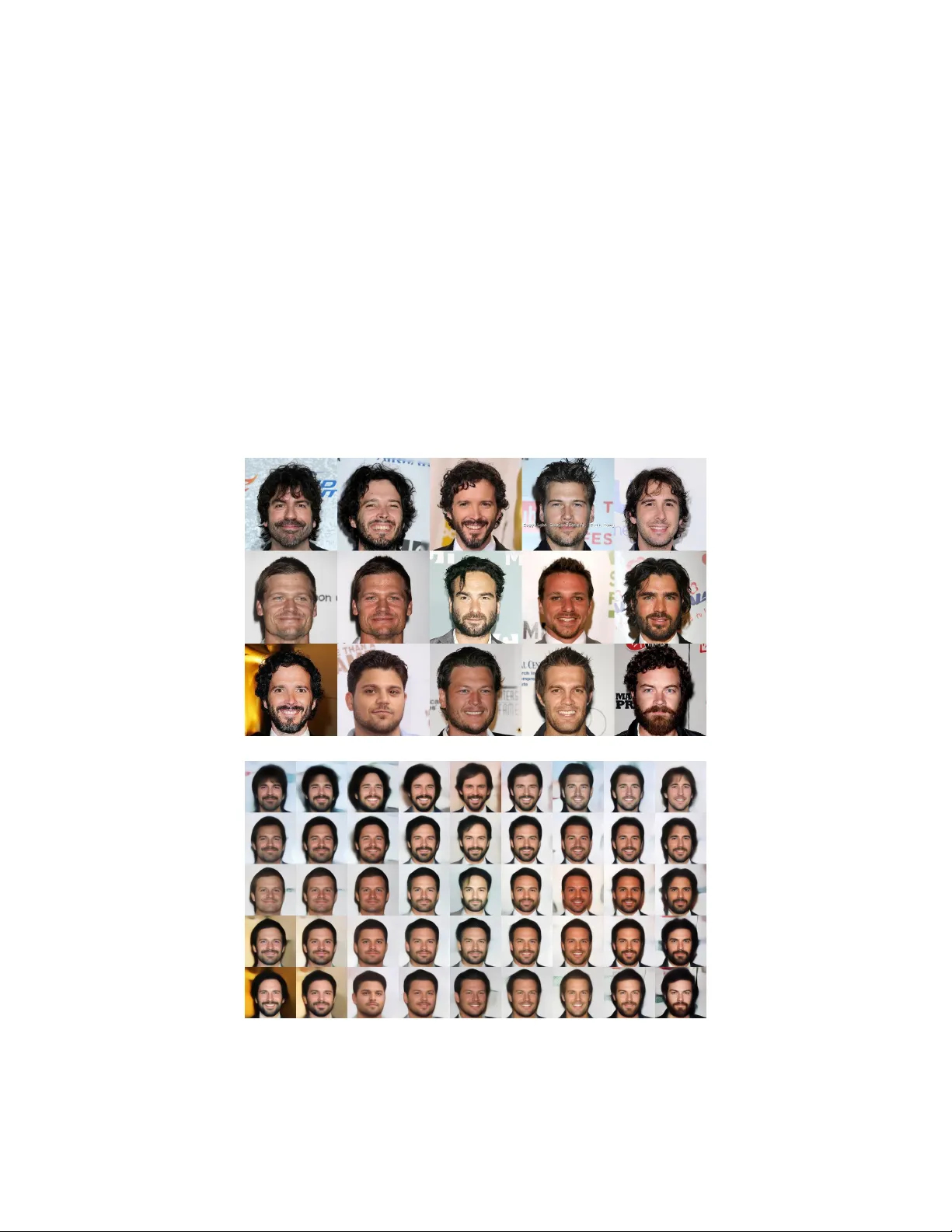
Sampling Generativ e Networks T om White School of Design V ictoria Univ ersity of W ellington W ellington, New Zealand tom.white@vuw.ac.nz Abstract W e introduce sev eral techniques for sampling and visualizing the latent spaces of generati ve models. Replacing linear interpolation with spherical linear interpolation prev ents diver ging from a model’ s prior distrib ution and produces sharper samples. J-Diagrams and MINE grids are introduced as visualizations of manifolds created by analogies and nearest neighbors. W e demonstrate two new techniques for deri ving attrib ute v ectors: bias-corrected v ectors with data replication and synthetic vectors with data augmentation. Binary classification using attribute vectors is presented as a technique supporting quantitativ e analysis of the latent space. Most techniques are intended to be independent of model type and examples are sho wn on both V ariational Autoencoders and Generati ve Adversarial Networks. 1 Introduction Generativ e models are a popular approach to unsupervised machine learning. Generati ve neural network models are trained to produce data samples that resemble the training set. Because the number of model parameters is significantly smaller than the training data, the models are forced to discover ef ficient data representations. These models are sampled from a set of latent v ariables in a high dimensional space, here called a latent space. Latent space can be sampled to generate observable data values. Learned latent representations often also allo w semantic operations with vector space arithmetic (Figure 1). Figure 1: Schematic of the latent space of a generati ve model. In the general case, a generati ve model includes an encoder to map from the feature space (here images of f aces) into a high dimensional latent space. V ector space arithmetic can be used in the latent space to perform semantic operations. The model also includes a decoder to map from the latent space back into the feature space, where the semantic operations can be observ ed. If the latent space transformation is the identity function we refer to the encoding and decoding as a reconstruction of the input through the model. 30th Conference on Neural Information Processing Systems (NIPS 2016), Barcelona, Spain. Generativ e models are often applied to datasets of images. T wo popular generati ve models for image data are the V ariational Autoencoder (V AE, Kingma & W elling, 2014) and the Generati ve Adv ersarial Network (GAN, Goodfellow et al., 2014). V AEs use the framew ork of probabilistic graphical models with an objecti ve of maximizing a lo wer bound on the likelihood of the data. GANs instead formalize the training process as a competition between a generati ve network and a separate discriminativ e network. Though these two framew orks are very dif ferent, both construct high dimensional latent spaces that can be sampled to generate images resembling training set data. Moreov er , these latent spaces are generally highly structured and can enable complex operations on the generated images by simple vector space arithmetic in the latent space (Larsen et al., 2016). Generativ e models are be ginning to find their w ay out of academia and into creati ve applications. In this paper we present techniques for improving the visual quality of generati ve models that are generally independent of the model itself. These include spherical linear interpolation, visualizing analogies with J-diagrams, and generating local manifolds with MINE grids. These techniques can be combined generate low dimensional embeddings of images close to the trained manifold. These can be used for visualization and creating realistic interpolations across latent space. Also by standardizing these operations independent of model type, the latent space of different generativ e models are more directly comparable with each other, e xposing the strengths and weaknesses of various approaches. Additionally , two ne w techniques for b uilding latent space attribute vectors are introduced. On labeled datasets with correlated labels, data replication can be used to create bias-corrected v ectors. Synthetic attributes v ectors also can be deriv ed via data augmentation on unlabeled data. Quantitative analysis of attribute v ectors can be performed by using them as the basis for attribute binary classifiers. 2 Sampling T echniques Generativ e models are often ev aluated by examining samples from the latent space. T echniques frequently used are random sampling and linear interpolation. But often these can result in sampling the latent space from locations very far outside the manifold of probable locations. Our work has follo wed two useful principles when sampling the latent space of a generativ e model. The first is to av oid sampling from locations that are highly unlikely giv en the prior of the model. This technique is very well established - including being used in the original V AE paper which adjusted sampling through the inv erse CDF of the Gaussian to accommodate the Gaussian prior (Kingma & W elling, 2014). The second principle is to recognize that the dimensionality of the latent space is often artificially high and may contains dead zones that are not on the manifold learned during training. This has been demonstrated for V AE models (Makhzani et al., 2016) and implies that simply matching the model’ s prior will not always be suf ficient to yield samples that appear to have been drawn from the training set. 2.1 Interpolation Interpolation is used to trav erse between two known locations in latent space. Research on gener - ativ e models often uses interpolation as a way of demonstrating that a generativ e model has not simply memorized the training e xamples (eg: Radford et al., 2015, §6.1). In creativ e applications interpolations can be used to provide smooth transitions between two decoded images. Frequently linear interpolation is used, which is easily understood and implemented. But this is often inappropriate as the latent spaces of most generative models are high dimensional (> 50 dimensions) with a Gaussian or uniform prior . In such a space, linear interpolation tra verses locations that are extremely unlik ely giv en the prior . As a concrete example, consider a 100 dimensional space with the Gaussian prior µ =0, σ =1. Here all random vectors will generally a length very close to 10 (standard deviation < 1). Howe ver , linearly interpolating between any two will usually result in a "tent-pole" effect as the magnitude of the v ector decreases from roughly 10 to 7 at the midpoint, which is o ver 4 standard deviations a way from the expected length. 2 Our proposed solution is to use spherical linear interpolation slerp instead of linear interpolation. W e use a formula introduced by (Shoemak e 85) in the context of great arc inbetweening for rotation animations: This treats the interpolation as a great circle path on an n-dimensional hypersphere (with elev ation changes). This technique has sho wn promising results on both V AE and GAN generativ e models and with both uniform and Gaussian priors (Figure 2). Figure 2: DCGAN (Radford 15) interpolation pairs with identical endpoints and uniform prior . In each pair , the top series is linear interpolation and the bottom is spherical. Note the weak generations produced by linear interpolation at the center , which are not present in spherical interpolation. 2.2 Analogy Analogy has been sho wn to capture regularities in continuous space models. In the latent space of some linguistic models “King – Man + W oman” results in a vector very close to “Queen” (Mikolo v et al., 2013). This technique has also been used in the context of deep generati ve models to solv e visual analogies (Reed et al., 2015). Analogies are usually written in the form: A : B :: C :? Such a formation answers the question “What is the result of applying the transformation A:B to C?” In a vector space the solution generally proposed is to solv e the analogy using vector math: ( B − A ) = (? − C ) ? = C + B − A Note that an interesting property of this solution is an implied symmetry: A : C :: B :? 3 Because the same terms can be rearranged: ( C − A ) = (? − B ) ? = B + C − A Generativ e models that include an encoder for computing latent vectors giv en new samples allo w for visual analogies. W e have de vised a visual representation for depicting analogies of visual generative networks called a “J-Diagram”. The J- Diagram uses interpolation across two dimensions two e xpose the manifold of the analogy . It also makes the symmetric nature of the analogy clear (Figure 3). The J-Diagram also serves as a reference visualization across dif ferent model settings because it is deterministically generated from images which can be held constant. This makes it a useful tool for comparing results across epochs during training, after adjusting hyperparameters, or e ven across completely different model types (Figure 4). Figure 3: J-Diagram. The three corner images are inputs to the system, with the top left being the “source” (A) and the other two being “analogy targets” (B and C). Adjacent to each is the reconstruction resulting from running the image through both the encoder and decoder of the model. The bottom right image shows the result of applying the analogy operation (B + C) – A. All other images are interpolations using the slerp operator . (model: V AE from Lamb 16 on CelebA) Figure 4: Same J-Diagram repeated with dif ferent model type. T o facilitate comparisons (and demonstrate results are not cherry-picked) inputs selected are the first 3 images of the v alidation set. (model: GAN from Dumoulin 16 on CelebA) 4 2.3 Manifold T raversal Generati ve models can produce a latent space that is not tightly packed, and the dimensionality of the latent space is often set artificially high. As a result, the manifold of trained e xamples is can be a subset of the latent space after training, resulting in dead zones in the expected prior . If the model includes an encoder, one simple way to stay on the manifold is by only using out of sample encodings (ie: any data not used in training) in the latent space. This is a useful diagnostic, but is o verly restricti ve in a creativ e application context since it pre vents the model from suggesting new and nov el samples from the model. Howe ver , we can recover this ability by also including the results of operations on these encoded samples that stay close to the manifold, such as interpolation, extrapolation, and analogy generation. Ideally , there would be a mechanism to disco ver this manifold within the latent space. In generativ e models with an encoder and ample out-of-sample data, we can instead precompute locations on the manifold with suf ficient density , and later query for nearby points in the latent space from this known set. This offers a navigation mechanism based on hopping to nearest neighbors across a large database of encoded samples. When combined with interpolation, we call this visualization a Manifold Interpolated Neighbor Embedding (MINE). A MINE grid is useful to visualize local patches of the latent space (Figure 5). (a) Nearest Neighbors are found and embedded into a two dimensional grid. (b) Reconstructions are spread with interpolation to expose areas between them. Figure 5: Example of local V AE manifold built using the 30k CelebA validation and test images as a dataset of out of sample features. The resulting MINE grid represents a small contiguous manifold of the larger latent space. (model: V AE from Lamb 16 on CelebA) 5 3 Attribute V ectors Many generati ve models result in a latent space that is highly structured, ev en on purely unsupervised datasets (Radford et al., 2015). When combined with labeled data, attribute vectors can be computed using simple arithmetic. For example, a vector can be computed which represents the smile attribute, which by shorthand we call a smile v ector . Following (Larsen et al., 2016), the smile vector can be computed by simply subtracting the mean v ector for images without the smile attribute from the mean vector for images with the smile attribute. This smile vector can then be applied to in a positive or negati ve direction to manipulate this visual attribute on samples taken from latent space (Figure 6). Figure 6: Tra versals along the smile vector . (model: GAN from Dumoulin 16 on CelebA) 3.1 Correlated Labels The approach of building attrib ute vectors from means of labeled data has been noted to suffer from correlated labels (Larsen et al., 2016). While many correlations w ould be expected from ground truths (eg: heavy makeup and wearing lipstick) we discov ered others that appear to be from sampling bias. For example, male and smiling attrib utes hav e unexpected neg ativ e correlations because women in the CelebA dataset are much more likely to be smiling than men. (T able 1). Male Not Male T otal Smiling 17% 31% 48% Not Smiling 25% 27% 52% T otal 42% 58% T able 1: Breakdown of CelebA smile versus male attributes. In the total population the smile attrib ute is almost balanced (48% smile). But separating the data further shows that those with the male attribute smile only 42% of the time while those without it smile 58% of the time. Figure 7: Initial attempts to b uild a smile vector suf fered from sampling bias. The effect was that removing smiles from reconstructions (left) also added male attributes (center). By using replication to balance the data across both attributes before computing the attribute v ectors, the gender bias was remov ed (right). (model: V AE from Lamb 16 on CelebA) 6 In an online service we setup to automatically add and remov e smiles from images 1 , we discov ered this gender bias was visually evident in the results. Our solution was to use replication on the training data such that the dataset was balanced across attributes. This was effecti ve because ultimately the vectors are simply summed together when computing the attrib ute vector (Figure 7). This balancing technique can also be applied to attributes correlated due to ground truths. Decoupling attributes allo ws individual ef fects to be applied separately . As an example, the two attrib utes smiling and mouth open are highly correlated in the CelebA training set (T able 2). This is not surprising, as physically most people photographed smiling would also ha ve their mouth open. Howe ver by forcing these attributes to be balanced, we can construct two decoupled attrib ute vectors. This allows for more flexibility in applying each attrib ute separately to varying degrees (Figure 8). Open Mouth Not Open Mouth T otal Smiling 36% 12% 48% Not Smiling 12% 40% 52% T otal 48% 52% T able 2: CelebA smile versus open mouth attrib utes shows a strong symmetric correlation (greater than 3 to 1). Figure 8: Decoupling attribute vectors for smiling (x-axis) and mouth open (y-axis) allo ws for more flexible latent space transformations. Input shown at left with reconstruction adjacent. (model: V AE from Lamb 16 on CelebA) 3.2 Synthetic Attrib utes It has been noted that samples drawn from V AE based models is that they tend to be blurry (Goodfel- low et al., 2014; Larsen et al., 2015). A possible solution to this would be to disco ver an attribute vector for “unblur”, and then apply this as a constant offset to latent vectors before decoding. CelebA includes a blur label for each image, and so a blur attribute vector was computed and then e xtrapolated in the negati ve direction. This was found to noticeably reduce blur , but also resulted in a number of unwanted artifacts such as increased image brightness. W e concluded this to be the result of human bias in labeling. Labelers appear more likely to label darker images as blurry , so this unblur vector was found to suffer from attrib ute correlation that also “lightened” the reconstruction. This bias could not be easily corrected because CelebA does not include a brightness label for rebalancing the data. For the blurring attribute, an algorithmic solution is a vailable. W e take a large set of images from the training set and process them through a Gaussian blur filter (figure 9). Then we run both the original image set and the blurred image set through the encoder and subtract the means of each set to compute a new attrib ute vector for blur . W e call this a synthetic attribute vector because this label 1 https://twitter.com/smilevector 7 Figure 9: Zoomed detail from training images (top) and computed blurred images (bottom) were both encoded in order to determine a non-biased blur attribute v ector . is deriv ed from algorithmic data augmentation of the training set. This technique removes the labeler bias, is straightforward to implement, and resulted in samples closely resembling the reconstructions with less noticeable blur (figure 10). Figure 10: Zoomed detail of images from the validation set (top) are reconstructed (second row). Applying an offset in latent space based on the CelebA blur attribute (third ro w) does reduce noticeable blur from the reconstructions, b ut introduces visual artifacts including brightening due to attribute correlation. Applying an attribute vector instead computed from synthetic blur (bottom) yields images noticeably deblurred from the reconstructions and without unrelated artifacts. 3.3 Quantitative Analysis with Classicication The results of applying attrib ute vectors visually to images are often quite striking. But it would be useful to be able to e valuate the relati ve ef ficacy of v arious attribute vectors to each other or across dif ferent models and hyperparamaters. Attribute vectors ha ve potential to be widely applicable outside of images in domain specific latent spaces, and this provides additional challenges for quantifying their performance. For example, recent work has sho wn the ability to use latent space model as a continuous representation of molecules (Gómez 16); though it is straightforward to generate vectors for attributes such as solubility in these spaces, the ev aluation of these operations to existing molecules would appear to require specific domain kno wledge. 8 Approach / Attribute [1] [2] W [2] L [3] ANet [4] LNet [4] Full V AE AtDot GAN AtDot 5 O.C. Shadow 85 82 88 86 88 91 88 89 Arched Eyebrow 76 73 78 75 74 79 75 75 Attractiv e 78 77 81 79 77 81 71 69 Bags Under Eye 76 71 79 77 73 79 80 79 Bald 89 92 96 92 95 98 98 98 Bangs 88 89 92 94 92 95 90 90 Big Lips 64 61 67 63 66 68 85 76 Big Nose 74 70 75 74 75 78 77 77 Black Hair 70 74 85 77 84 88 83 81 Blond Hair 80 81 93 86 91 95 87 90 Blurry 81 77 86 83 80 84 95 95 Brown Hair 60 69 77 74 78 80 76 81 Bushy Eyebro w 80 76 86 80 85 90 87 86 Chubby 86 82 86 86 86 91 94 94 Double Chin 88 85 88 90 88 92 95 95 Eyeglasses 98 94 98 96 96 99 95 94 Goatee 93 86 93 92 92 95 93 94 Gray Hair 90 88 94 93 93 97 95 96 Heavy Mak eup 85 84 90 87 85 90 76 75 High Cheekbone 84 80 86 85 84 87 81 68 Male 91 93 97 95 94 98 81 80 Mouth Open 87 82 93 85 86 92 78 67 Mustache 91 83 93 87 91 95 95 96 Narrow Eyes 82 79 84 83 77 81 93 89 No Beard 90 87 93 91 92 95 85 84 Oval F ace 64 62 65 65 63 66 72 71 Pale Skin 83 84 91 89 87 91 96 96 Pointy Nose 68 65 71 67 70 72 72 72 Recede Hair 76 82 85 84 85 89 93 92 Rosy Cheeks 84 81 87 85 87 90 93 93 Sideburns 94 90 93 94 91 96 94 94 Smiling 89 89 92 92 88 92 87 68 Straight Hair 63 67 69 70 69 73 80 79 W avy Hair 73 76 77 79 75 80 75 75 Earring 73 72 78 77 78 82 81 81 Hat 89 91 96 93 96 99 96 97 Lipstick 89 88 93 91 90 93 79 77 Necklace 68 67 67 70 68 71 88 88 Necktie 86 88 91 90 86 93 93 92 Y oung 80 77 84 81 83 87 78 81 A verage 81 79 85 83 83 87 86 84 T able 3: A verage Classification Accurac y on the CelebA dataset. Models for both V AE AtDot and GAN AtDot use unsupervised training with attribute vectors computed on the training set data after model training w as completed. V AE AtDot from Lamb 16 with discriminative regularization disabled and GAN AtV ec from Dumoulin 16. Other results are [1] Kumar 08, [2] Zhang 14, [3] Li 13, and [4] LeCun 94 as reported in Ehrlich 16. 9 (a) Dot product. (b) Histogram. (c) R OC curve. Figure 11: Example of using an attribute vector for classification. A smile vector is first constructed in latent space from labeled training data. By taking the dot product of this smile vector with the encoded representation of any face, a scalar smile score is generated (a). This score can be the basis for a binary classifier . The histogram shows the distribution of positiv e (green) and negativ e (red) scores on the CelebA v alidation set (b). The ROC curve for a smile v ector based binary classifier is also shown (c). W e have found that very ef fective classifiers can be built in latent space using the dot product of an encoded vector with a computed attrib ute vector (figure 11A, 11B). W e hav e named this technique for building classifiers on latent spaces AtDot, and models trained on unsupervised data have been shown to produce strong results on CelebA across most attributes (table 3). Importantly , these binary classifiers provide a quantitati ve basis to ev aluate attribute vectors on a related surrogate task - their ability to be the basis for a simple linear classifier . This task is one of the most established paradigms in machine learning and provides a set of established tools such as R OC curves for offering ne w insights into the behavior of the attribute v ectors across different hyperparameters or dif ferent models (figure 11C). 4 Future W ork Software to support most techniques presented in this paper is included in a python softw are library that can be used with v arious generati ve models 2 . W e hope to continue to improve the library so that the techniques are applicable across a broad range of generativ e models. Attribute vector based classifiers also of fer a promising w ay to e valuate the suitability of attribute v ectors in domains outside of images. W e are inv estigating constructing a specially constructed prior on the latent space such that interpola- tions could be linear . This would simplify many of the latent space operations and might enable new types of operations. Giv en sufficient test data, the extent to which an encoded dataset de viates from the expected prior should be quantifiable. Developing such a metric w ould be useful in understanding the structure of the diff erent latent spaces including probability that random samples fall outside of the expected manifold of encoded data. Acknowledgments I am thankful for the constructiv e feedback from readers including Ehud Ben-Reuven, Zachary Lipton, and Alex Champandard. I thank V ictoria Univ ersity of W ellington School of Design for supporting research on Creati ve Intelligence. I also thank the vibrant machine learning and creati ve coding communities on twitter for their support and encouragement. References Dumoulin, V incent, Belghazi, Ishmael, Poole, Ben, Lamb, Alex, Arjovsky , Martin, Mastropietro, Olivier Courville, Aaron. Adversarially Learned Inference. https://arxiv.org/abs/1606.00704 2016 Ehrlich, Max, Shields, T imothy J., Almaev , Timur , Amer, Mohamed R. Facial Attrib utes Classification Using Multi-T ask Representation Learning. The IEEE Conference on Computer V ision and Pattern Recognition (CVPR) W orkshops. 2016. 2 https://github.com/dribnet/plat 10 Goodfellow , Ian, Pouget-Abadie, Jean, Mirza, Mehdi, Xu, Bing, W arde- Farley , David, Ozair , Sherjil, Courville, Aaron, and Bengio, Y oshua. Generati ve adversarial nets. In Ghahramani, Z., W elling, M., Cortes, C., Lawrence, N.D., and W einberger , K.Q. (eds.), Advances in Neural Information Processing Systems 27, pp. 2672–2680. Curran Associates, Inc., 2014. Gómez-Bombarelli, Rafael, Duv enaud, David, Miguel, Hernández-Lobato, José, Aguilera-Iparraguirre, Jor ge, Hirzel, T imothy D., Adams, Ryan P ., and Alán Aspuru-Guzik. Automatic chemical design using a data-dri ven continuous representation of molecules. https://arxiv.org/abs/1610.02415 2016 Kingma, Diederik P . and W elling, Max. Auto-encoding variational Bayes. In Proceedings of the International Conference on Learning Representations, 2014. Kumar , N., Belhumeur, P ., and Nayar , S. Facetracer: A search engine for large collections of images with f aces. In ECCV , 2008. Lamb, Alex, Dumoulin, V incent, Courville, Aaron. Discriminati ve Regularization for Generative Models. http://arxiv.org/abs/1602.03220 2016 Larsen, Anders Boesen Lindbo, Sønderby , Søren Kaae, Larochelle, Hugo, W inther, Ole. Autoencoding beyond pixels using a learned similarity metric. https://arxiv.org/abs/1512.09300 2016 LeCun, Y . and Bengio., Y . W ord-le vel training of a handwritten word recognizer based on con volutional neural networks. In ICPR, 1994. Li, J., and Zhang, Y . Learning surf cascade for fast and accurate object detection. In CVPR, 2013. Makhzani, Alireza, Shlens, Jonathon, Jaitly , Navdeep, Goodfellow , Ian, Brendan, Frey . Adversarial Autoen- coders. . 2016. Mikolov , T omas, Y ih, Scott W en-tau, Zweig, Geoffre y . Linguistic Regularities in Continuous Space W ord Representations. NAA CL-HL T , 2013. Radford , Alec, Metz , Luk e, Chintala, Soumith. Unsupervised Representation Learning with Deep Con volutional Generativ e Adversarial Networks. Advances in Neural Information Processing Systems, 2015. Reed, Scott E, Zhang, Y i, Zhang, Y uting, and Lee, Honglak. Deep visual analogy-making. In Cortes, C., Lawrence, N.D., Lee, D.D., Sugiyama, M., Garnett, R., and Garnett, R. (eds.), Adv ances in Neural Information Processing Systems 28, pp. 1252–1260. Curran Associates, Inc., 2015 Shoemake, K en. Animating rotation with quaternion curv es. In A CM Siggraph, 19(3):245–254, 1985. Zhang, N., Paluri, M., Ranzato, M., Darrell, T ., and Bourdev , L. Panda: Pose aligned networks for deep attribute modeling. In CVPR, 2014. 11