Alternating Back-Propagation for Generator Network

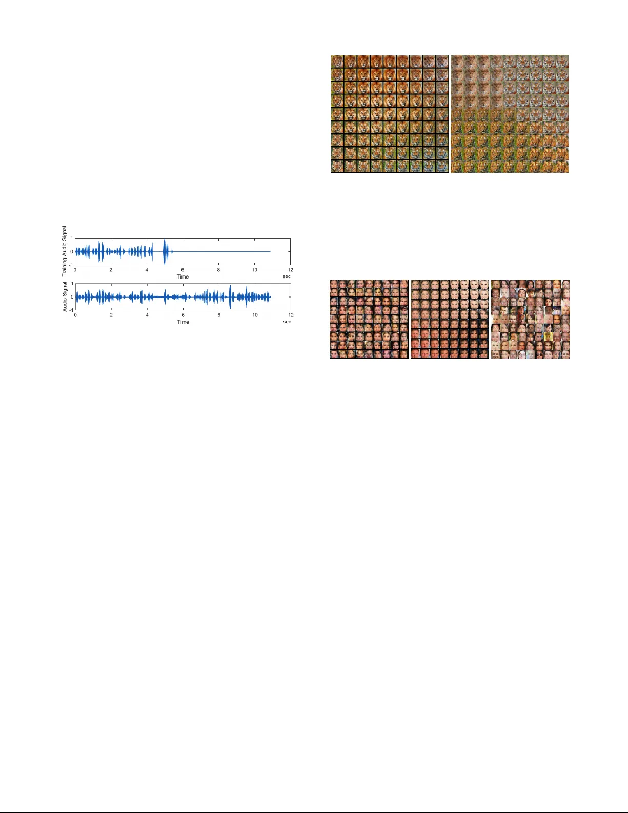
Alternating Back-Pr opagation for Generator Network Tian Han † , Y ang Lu † , Song-Chun Zhu, Y ing Nian W u Department of Statistics, Univ ersity of California, Los Angeles, USA Abstract This paper proposes an alternating back-propagation algorithm for learning the generator network model. The model is a non- linear generalization of f actor analysis. In this model, the map- ping from the continuous latent factors to the observed signal is parametrized by a con v olutional neural network. The alter - nating back-propagation algorithm iterates the following tw o steps: (1) Infer ential back-pr opagation , which infers the latent factors by Lange vin dynamics or gradient descent. (2) Learn- ing back-pr opagation , which updates the parameters given the inferred latent factors by gradient descent. The gradient computations in both steps are powered by back-propag ation, and they share most of their code in common. W e show that the alternating back-propagation algorithm can learn realis- tic generator models of natural images, video sequences, and sounds. Moreo v er , it can also be used to learn from incomplete or indirect training data. 1 Introduction This paper studies the fundamental problem of learning and inference in the generator network (Goodfellow et al . , 2014), which is a generativ e model that has become popular recently . Specifically , we propose an alternating back-propagation al- gorithm for learning and inference in this model. 1.1 Non-linear factor analysis The generator network is a non-linear generalization of factor analysis. Factor analysis is a prototype model in unsuper- vised learning of distrib uted representations. There are two directions one can pursue in order to generalize the factor analysis model. One direction is to generalize the prior model or the prior assumption about the latent factors. This led to methods such as independent component analysis (Hyväri- nen, Karhunen, and Oja, 2004), sparse coding (Olshausen and Field, 1997), non-negati ve matrix factorization (Lee and Seung, 2001), matrix factorization and completion for recom- mender systems (K oren, Bell, and V olinsky, 2009), etc. The other direction to generalize the factor analysis model is to generalize the mapping from the continuous latent fac- tors to the observed signal. The generator network is an example in this direction. It generalizes the linear mapping in factor analysis to a non-linear mapping that is defined by † Equal contributions. a con v olutional neural netw ork (Con vNet or CNN) (LeCun et al . , 1998; Krizhevsk y , Sutske ver , and Hinton, 2012; Doso- vitskiy , Springenberg, and Brox, 2015). It has been shown recently that the generator network is capable of generating realistic images (Denton et al . , 2015; Radford, Metz, and Chintala, 2016). The generator network is a fundamental representation of knowledge, and it has the follo wing properties: (1) Analysis : The model disentangles the variations in the observed signals into independent variations of latent factors. (2) Synthesis : The model can synthesize ne w signals by sampling the f ac- tors from the kno wn prior distribution and transforming the factors into the signal. (3) Embedding : The model embeds the high-dimensional non-Euclidean manifold formed by the observed signals into the low-dimensional Euclidean space of the latent factors, so that linear interpolation in the low- dimensional factor space results in non-linear interpolation in the data space. 1.2 Alternating back-propagation The factor analysis model can be learned by the Rubin-Thayer EM algorithm (Rubin and Thayer, 1982; Dempster, Laird, and Rubin, 1977), where both the E-step and the M-step are based on multiv ariate linear regression. Inspired by this algo- rithm, we propose an alternating back-propagation algorithm for learning the generator network that iterates the following two-steps: (1) Infer ential back-pr opagation : For each training e xam- ple, infer the continuous latent factors by Langevin dynamics or gradient descent. (2) Learning back-pr opagation : Update the parameters giv en the inferred latent factors by gradient descent. The Lange vin dynamics (Neal, 2011) is a stochastic sam- pling counterpart of gradient descent. The gradient computa- tions in both steps are powered by back-propagation. Because of the ConvNet structure, the gradient computation in step (1) is actually a by-product of the gradient computation in step (2) in terms of coding. Giv en the factors, the learning of the ConvNet is a su- pervised learning problem (Doso vitskiy , Springenberg, and Brox, 2015) that can be accomplished by the learning back- propagation. W ith factors unknown, the learning becomes an unsupervised problem, which can be solved by adding the inferential back-propagation as an inner loop of the learning 1 process. W e shall show that the alternating back-propagation algorithm can learn realistic generator models of natural im- ages, video sequences, and sounds. The alternating back-propagation algorithm follo ws the tradition of alternating operations in unsupervised learning, such as alternating linear regression in the EM algorithm for factor analysis, alternating least squares algorithm for matrix factorization (K oren, Bell, and V olinsky, 2009; Kim and Park, 2008), and alternating gradient descent algorithm for sparse coding (Olshausen and Field, 1997). All these unsupervised learning algorithms alternate an inference step and a learning step, as is the case with alternating back-propagation. 1.3 Explaining-away inference The inferential back-propagation solv es an inv erse problem by an explaining-aw ay process, where the latent factors com- pete with each other to explain each training example. The following are the advantages of the explaining-aw ay infer- ence of the latent factors: (1) The latent factors may follo w sophisticated prior mod- els. For instance, in te xtured motions (W ang and Zhu, 2003) or dynamic textures (Doretto et al . , 2003), the latent factors may follow a dynamic model such as v ector auto-regression. By inferring the latent factors that explain the observed ex- amples, we can learn the prior model. (2) The observed data may be incomplete or indirec t. For instance, the training images may contain occluded objects. In this case, the latent factors can still be obtained by explain- ing the incomplete or indirect observations, and the model can still be learned as before. 1.4 Learning from incomplete or indirect data W e venture to propose that a main adv antage of a generativ e model is to learn from incomplete or indirect data, which are not uncommon in practice. The generative model can then be ev aluated based on how well it recov ers the unobserved original data, while still learning a model that can generate new data. Learning the generator network from incomplete data can be considered a non-linear generalization of matrix completion. W e also propose to ev aluate the learned generator network by the reconstruction error on the testing data. 1.5 Contribution and related work The main contribution of this paper is to propose the alter- nating back-propagation algorithm for training the generator network. Another contrib ution is to ev aluate the generativ e models by learning from incomplete or indirect training data. Existing training methods for the generator network av oid explain-a way inference of latent factors. T wo methods have recently been devised to accomplish this. Both methods in- volv e an assisting network with a separate set of parameters in addition to the original network that generates the sig- nals. One method is variational auto-encoder (V AE) (Kingma and W elling, 2014; Rezende, Mohamed, and Wierstra, 2014; Mnih and Gre gor, 2014), where the assisting network is an in- ferential or recognition network that seeks to approximate the posterior distribution of the latent factors. The other method is the generativ e adversarial network (GAN) (Goodfellow et al . , 2014; Denton et al . , 2015; Radford, Metz, and Chintala, 2016), where the assisting network is a discriminator netw ork that plays an adversarial role against the generator netw ork. Unlike alternating back-propagation, V AE does not per- form explicit explain-aw ay inference, while GAN avoids inferring the latent factors altogether . In comparison, the al- ternating back-propagation algorithm is simpler and more basic, without resorting to an e xtra network. While it is dif- ficult to compare these methods directly , we illustrate the strength of alternating back-propagation by learning from incomplete and indirect data, where we only need to explain whatev er data we are giv en. This may prove dif ficult or less con venient for V AE and GAN. Meanwhile, alternating back-propagation is complemen- tary to V AE and GAN training. It may use V AE to initialize the inferential back-propagation, and as a result, may im- prov e the inference in V AE. The inferential back-propagation may help infer the latent f actors of the observ ed examples for GAN, thus providing a method to test if GAN can explain the entire training set. The generator network is based on a top-down Con vNet. One can also obtain a probabilistic model based on a bottom- up Con vNet that defines descriptiv e features (Xie et al . , 2016; Lu, Zhu, and W u, 2016). 2 F actor analysis with Con vNet 2.1 F actor analysis and beyond Let Y be a D -dimensional observed data vector , such as an image. Let Z be the d -dimensional vector of continuous latent factors, Z = ( z k , k = 1 , ..., d ) . The traditional fac- tor analysis model is Y = W Z +  , where W is D × d matrix, and  is a D -dimensional error vector or the observ a- tional noise. W e assume that Z ∼ N(0 , I d ) , where I d stands for the d -dimensional identity matrix. W e also assume that  ∼ N(0 , σ 2 I D ) , i.e., the observational errors are Gaussian white noises. There are three perspectives to view W . (1) Basis vectors . Write W = ( W 1 , ..., W d ) , where each W k is a D -dimensional column vector . Then Y = P d k =1 z k W k +  , i.e., W k are the basis vectors and z k are the coef ficients. (2) Loading matrix . Write W = ( w 1 , ..., w D ) > , where w > j is the j -th ro w of W . Then y j = h w j , Z i +  j , where y j and  j are the j -th components of Y and  respectiv ely . Each y j is a loading of the d factors where w j is a vector of loading weights, indicating which factors are important for determin- ing y j . W is called the loading matrix. (3) Matrix factoriza- tion . Suppose we observe Y = ( Y 1 , ..., Y n ) , whose factors are Z = ( Z 1 , ..., Z n ) , then Y ≈ W Z . The factor analysis model can be learned by the Rubin- Thayer EM algorithm, which in volves alternating re gressions of Z on Y in the E-step and of Y on Z in the M-step, with both steps po wered by the sweep operator (Rubin and Thayer, 1982; Liu, Rubin, and W u, 1998). The factor analysis model is the prototype of many sub- sequent models that generalize the prior model of Z . (1) Independent component analysis (Hyvärinen, Karhunen, and Oja, 2004), d = D ,  = 0 , and z k are assumed to follow independent heavy tailed distributions. (2) Sparse coding 2 (Olshausen and Field, 1997), d > D , and Z is assumed to be a redundant but sparse vector , i.e., only a small number of z k are non-zero or significantly different from zero. (3) Non-ne gative matrix factorization (Lee and Seung, 2001), it is assumed that z k ≥ 0 . (4) Recommender system (K oren, Bell, and V olinsky, 2009), Z is a v ector of a customer’ s de- sires in different aspects, and w j is a vector of product j ’ s desirabilities in these aspects. 2.2 Con vNet mapping In addition to generalizing the prior model of the latent f ac- tors Z , we can also generalize the mapping from Z to Y . In this paper , we consider the generator network model (Good- fellow et al . , 2014) that retains the assumptions that d < D , Z ∼ N(0 , I d ) , and  ∼ N(0 , σ 2 I D ) as in traditional fac- tor analysis, but generalizes the linear mapping W Z to a non-linear mapping f ( Z ; W ) , where f is a Con vNet, and W collects all the connection weights and bias terms of the Con vNet. Then the model becomes Y = f ( Z ; W ) + , Z ∼ N(0 , I d ) ,  ∼ N(0 , σ 2 I D ) , d < D . (1) The reconstruction error is || Y − f ( Z ; W ) || 2 . W e may as- sume more sophisticated models for  , such as colored noise or non-Gaussian texture. If Y is binary , we can emit Y by a probability map P = 1 / [1 + exp( − f ( Z ; W ))] , where the sigmoid transformation and Bernoulli sampling are carried out pixel-wise. If Y is multi-level, we may assume multi- nomial logistic emission model or some ordinal emission model. Although f ( Z ; W ) can be any non-linear mapping, the Con vNet parameterization of f ( Z ; W ) makes it particularly close to the original f actor analysis. Specifically , we can write the top-down Con vNet as follows: Z ( l − 1) = f l ( W l Z ( l ) + b l ) , (2) where f l is element-wise non-linearity at layer l , W l is the matrix of connection weights, b l is the vector of bias terms at layer l , and W = ( W l , b l , l = 1 , ..., L ) . Z (0) = f ( Z ; W ) , and Z ( L ) = Z . The top-down Con vNet (2) can be considered a recursion of the original factor analysis model, where the factors at the layer l − 1 are obtained by the linear superpo- sition of the basis vectors or basis functions that are column vectors of W l , with the factors at the layer l serving as the co- efficients of the linear superposition. In the case of Con vNet, the basis functions are shift-in variant v ersions of one another, like wa velets. See Appendix for an in-depth understanding of the model. 3 Alternating back-propagation If we observe a training set of data vectors { Y i , i = 1 , ..., n } , then each Y i has a corresponding Z i , but all the Y i share the same Con vNet W . Intuiti vely , we should infer { Z i } and learn W to minimize the reconstruction error P n i =1 || Y i − f ( Z i ; W ) || 2 plus a regularization term that corresponds to the prior on Z . More formally , the model can be written as Z ∼ p ( Z ) and [ Y | Z, W ] ∼ p ( Y | Z , W ) . Adopting the language of the EM algorithm (Dempster , Laird, and Rubin, 1977), the complete- data model is giv en by log p ( Y , Z ; W ) = log [ p ( Z ) p ( Y | Z, W )] = − 1 2 σ 2 k Y − f ( Z ; W ) k 2 − 1 2 k Z k 2 + const . (3) The observed-data model is obtained by integrating out Z : p ( Y ; W ) = R p ( Z ) p ( Y | Z , W ) d Z . The posterior distribu- tion of Z is gi ven by p ( Z | Y , W ) = p ( Y , Z ; W ) /p ( Y ; W ) ∝ p ( Z ) p ( Y | Z , W ) as a function of Z . For the training data { Y i } , the complete-data log- likelihood is L ( W , { Z i } ) = P n i =1 log p ( Y i , Z i ; W ) , where we assume σ 2 is giv en. Learning and inference can be ac- complished by maximizing the complete-data log-likelihood, which can be obtained by the alternating gradient descent algorithm that iterates the following tw o steps: (1) Inference step: update Z i by running l steps of gradient descent. (2) Learning step: update W by one step of gradient descent. A more rigorous method is to maximize the observed-data log-likelihood, which is L ( W ) = P n i =1 log p ( Y i ; W ) = P n i =1 log R p ( Y i , Z i ; W ) d Z i . The observed-data log- likelihood takes into account the uncertainties in inferring Z i . See Appendix for an in-depth understanding. The gradient of L ( W ) can be calculated according to the following well-kno wn fact that underlies the EM algorithm: ∂ ∂ W log p ( Y ; W ) = 1 P ( Y ; W ) ∂ ∂ W Z p ( Y , Z ; W ) d Z = E p ( Z | Y ,W )  ∂ ∂ W log p ( Y , Z ; W )  . (4) The expectation with respect to p ( Z | Y , W ) can be approxi- mated by drawing samples from p ( Z | Y , W ) and then com- puting the Monte Carlo av erage. The Langevin dynamics for sampling Z ∼ p ( Z | Y , W ) iterates Z τ +1 = Z τ + sU τ + s 2 2  1 σ 2 ( Y − f ( Z τ ; W )) ∂ ∂ Z f ( Z τ ; W ) − Z τ  , (5) where τ denotes the time step for the Lange vin sampling, s is the step size, and U τ denotes a random vector that follows N(0 , I d ) . The Lange vin dynamics (5) is an explain-away process, where the latent factors in Z compete to explain away the current residual Y − f ( Z τ ; W ) . T o explain Langevin dynamics, its continuous time ver - sion for sampling π ( x ) ∝ exp[ −E ( x )] is x t +∆ t = x t − ∆ t E 0 ( x t ) / 2 + √ ∆ tU t . The dynamics has π as its station- ary distribution, because it can be shown that for any well- behav ed testing function h , if x t ∼ π , then E[ h ( x t +∆ t )] − E[ h ( x t )] → 0 , as ∆ t → 0 , so that x t +∆ t ∼ π . Alter- nativ ely , giv en x t = x , suppose x t +∆ t ∼ K ( x, y ) , then [ π ( y ) K ( y , x )] / [ π ( x ) K ( x, y )] → 1 as ∆ t → 0 . The stochastic gradient algorithm of (Y ounes, 1999) can be used for learning, where in each iteration, for each Z i , only a single copy of Z i is sampled from p ( Z i | Y i , W ) by running a finite number of steps of Langevin dynamics starting from the current v alue of Z i , i.e., the warm start. W ith { Z i } sampled 3 in this manner , we can update the parameter W based on the gradient L 0 ( W ) , whose Monte Carlo approximation is: L 0 ( W ) ≈ n X i =1 ∂ ∂ W log p ( Y i , Z i ; W ) = − n X i =1 ∂ ∂ W 1 2 σ 2 k Y i − f ( Z i ; W ) k 2 = n X i =1 1 σ 2 ( Y i − f ( Z i ; W )) ∂ ∂ W f ( Z i ; W ) . (6) Algorithm 1 describes the details of the learning and sam- pling algorithm. Algorithm 1 Alternating back-propagation Require: (1) training examples { Y i , i = 1 , ..., n } (2) number of Langevin steps l (3) number of learning iterations T Ensure: (1) learned parameters W (2) inferred latent factors { Z i , i = 1 , ..., n } 1: Let t ← 0 , initialize W . 2: Initialize Z i , for i = 1 , ..., n . 3: repeat 4: Inferential back-propagation : For each i , run l steps of Langevin dynamics to sample Z i ∼ p ( Z i | Y i , W ) with w arm start, i.e., starting from the current Z i , each step follows equation (5). 5: Learning back-pr opagation : Update W ← W + γ t L 0 ( W ) , where L 0 ( W ) is computed according to equation (6), with learning rate γ t . 6: Let t ← t + 1 7: until t = T If the Gaussian noise U τ in the Lange vin dynamics (5) is remov ed, then the above algorithm becomes the alternating gradient descent algorithm. It is possible to update both W and { Z i } simultaneously by joint gradient descent. Both the inferential back-propagation and the learn- ing back-propagation are guided by the residual Y i − f ( Z i ; W ) . The inferential back-propagation is based on ∂ f ( Z ; W ) /∂ Z , whereas the learning back-propagation is based on ∂ f ( Z ; W ) /∂ W . Both gradients can be ef ficiently computed by back-propag ation. The computations of the two gradients share most of their steps. Specifically , for the top-down Con vNet defined by (2), ∂ f ( Z ; W ) /∂ W and ∂ f ( Z ; W ) /∂ Z share the same code for the chain rule com- putation of ∂ Z ( l − 1) /∂ Z ( l ) for l = 1 , ..., L . Thus, the code for ∂ f ( Z ; W ) /∂ Z is part of the code for ∂ f ( Z ; W ) /∂ W . In Algorithm 1, the Langevin dynamics samples from a gradually changing posterior distribution p ( Z i | Y i , W ) be- cause W keeps changing. The updating of both Z i and W col- laborate to reduce the reconstruction error k Y i − f ( Z i ; W ) || 2 . The parameter σ 2 plays the role of annealing or tempering in Lange vin sampling. If σ 2 is very lar ge, then the posterior is close to the prior N(0 , I d ) . If σ 2 is very small, then the posterior may be multi-modal, but the e volving ener gy land- scape of p ( Z i | Y i , W ) may help alle viate the trapping of the local modes. In practice, we tune the value of σ 2 instead of estimating it. The Langevin dynamics can be extended to Hamiltonian Monte Carlo (Neal, 2011) or more sophisticated versions (Girolami and Calderhead, 2011). 4 Experiments The code in our experiments is based on the MatCon vNet package of (V edaldi and Lenc, 2015). The training images and sounds are scaled so that the inten- sities are within the range [ − 1 , 1] . W e adopt the structure of the generator network of (Radford, Metz, and Chintala, 2016; Dosovitskiy , Springenberg, and Brox, 2015), where the top- do wn network consists of multiple layers of decon volution by linear superposition, ReLU non-linearity , and up-sampling, with tanh non-linearity at the bottom-layer (Radford, Metz, and Chintala, 2016) to make the signals fall within [ − 1 , 1] . W e also adopt batch normalization (Iof fe and Szegedy, 2015). W e fix σ = . 3 for the standard deviation of the noise vector  . W e use l = 10 or 30 steps of Langevin dynamics within each learning iteration, and the Langevin step size s is set at .1 or . 3 . W e run T = 600 learning iterations, with learning rate .0001, and momentum .5. The learning algorithm produces the learned netw ork parameters W and the inferred latent factors Z for each signal Y in the end. The synthesized signals are obtained by f ( Z ; W ) , where Z is sampled from the prior distribution N(0 , I d ) . 4.1 Qualitative experiments Figure 1: Modeling texture patterns. F or each example, Left: the 224 × 224 observed image. Right: the 448 × 448 generated image. Experiment 1. Modeling textur e patterns . W e learn a separate model from each texture image. The images are collected from the Internet, and then resized to 224 × 224. The synthesized images are 448 × 448. Figures 1 shows four examples. The f actors Z at the top layer form a √ d × √ d image, with each pixel following N(0 , 1) independently . The √ d × √ d 4 image Z is then transformed to Y by the top-down Con- vNet. W e use d = 7 2 in the learning stage for all the texture experiments. In order to obtain the synthesized image, we randomly sample a 14 × 14 Z from N (0 , I ) , and then expand the learned netw ork W to generate the 448 × 448 synthesized image f ( Z ; W ) . The training network is as follows. Starting from 7 × 7 image Z , the network has 5 layers of decon volution with 5 × 5 kernels (i.e., linear superposition of 5 × 5 basis functions), with an up-sampling factor of 2 at each layer (i.e., the basis functions are 2 pixels apart). The number of channels in the first layer is 512 (i.e., 512 translation in variant basis functions), and is decreased by a f actor 2 at each layer . The Langevin steps l = 10 with step size s = . 1 . Figure 2: Modeling sound patterns. Row 1: the waveform of the training sound (the range is 0-5 seconds). Row 2: the wa veform of the synthesized sound (the range is 0-11 sec- onds). Experiment 2. Modeling sound patterns . A sound signal can be treated as a one-dimensional texture image (McDer- mott and Simoncelli, 2011). The sound data are collected from the Internet. Each training signal is a 5 second clip with the sampling rate of 11025 Hertz and is represented as a 1 × 60000 vector . W e learn a separate model from each sound signal. The latent factors Z form a sequence that follows N (0 , I d ) , with d = 6 . The top-down network consists of 4 layers of decon volution with kernels of size 1 × 25 , and up-sampling factor of 10. The number of channels in the first layer is 256, and decreases by a factor of 2 at each layer . For synthesis, we start from a longer Gaussian white noise sequence Z with d = 12 and generate the synthesized sound by expanding the learned network. Figure 2 shows the wav eforms of the observed sound signal in the first row and the synthesized sound signal in the second row . Experiment 3. Modeling object patterns . W e model object patterns using the network structure that is essentially the same as the network for the texture model, except that we include a fully connected layer under the latent factors Z , no w a d -dimensional vector . The images are 64 × 64 . W e use ReLU with a leaking factor .2 (Maas, Hannun, and Ng, 2013; Xu et al . , 2015). The Langevin steps l = 30 with step size s = . 3 . In the first experiment, we learn a model where Z has two components, i.e., Z = ( z 1 , z 2 ) , and d = 2 . The training data are 11 images of 6 tigers and 5 lions. After training the model, we generate images using the learned top-down Con vNet for Figure 3: Modeling object patterns. Left: the synthesized images generated by our method. They are generated by f ( Z ; W ) with the learned W , where Z = ( z 1 , z 2 ) ∈ [ − 2 , 2] 2 , and Z is discretized into 9 × 9 values. Right: the synthesized images generated using Deep Con volutional Gen- erati ve Adversarial Net (DCGAN). Z is discretized into 9 × 9 values within [ − 1 , 1] 2 . Figure 4: Modeling object patterns. Left: each image gen- erated by our method is obtained by first sampling Z ∼ N(0 , I 100 ) and then generating the image by f ( Z ; W ) with the learned W . Middle: interpolation. The images at the four corners are reconstructed from the inferred Z vectors of four images randomly selected from the training set. Each image in the middle is obtained by first interpolating the Z vectors of the four corner images, and then generating the image by f ( Z ; W ) . Right: the synthesized images generated by DCGAN, where Z is a 100 dimension vector sampled from uniform distribution. ( z 1 , z 2 ) ∈ [ − 2 , 2] 2 , where we discretize both z 1 and z 2 into 9 equally spaced v alues. The left panel of Figure 3 displays the synthesized images on the 9 × 9 panel. In the second experiment, we learn a model with d = 100 from 1000 face images randomly selected from the CelebA dataset (Liu et al . , 2015). The left panel of Figure 4 displays the images generated by the learned model. The middle panel displays the interpolation results. The images at the four cor- ners are generated by the Z vectors of four images randomly selected from the training set. The images in the middle are obtained by first interpolating the Z ’ s of the four corner im- ages using the sphere interpolation (Dinh, Sohl-Dickstein, and Bengio, 2016) and then generating the images by the learned Con vNet. W e also provide qualitative comparison with Deep Con- volutional Generati ve Adversarial Net (DCGAN) (Good- fellow et al . , 2014; Radford, Metz, and Chintala, 2016). The right panel of Figure 3 shows the generated results 5 for the lion-tiger dataset using 2 -dimensional Z . The right panel of Figure 4 displays the generated results trained on 1000 aligned faces from celebA dataset, with d = 100 . W e use the code from https://github.com/carpedm20/ DCGAN- tensorflow , with the tuning parameters as in (Rad- ford, Metz, and Chintala, 2016). W e run T = 600 iterations as in our method. Experiment 4. Modeling dynamic patterns . W e model a textured motion (W ang and Zhu, 2003) or a dynamic tex- ture (Doretto et al . , 2 003) by a non-linear dynamic system Y t = f ( Z t ; W ) +  t , and Z t +1 = AZ t + η t , where we as- sume the latent factors follo w a vector auto-re gressive model, where A is a d × d matrix, and η t ∼ N(0 , Q ) is the innovation. This model is a direct generalization of the linear dynamic system of (Doretto et al . , 2003), where Y t is reduced to Z t by principal component analysis (PCA) via singular value decomposition (SVD). W e learn the model in two steps. (1) T reat { Y t } as independent examples and learn W and infer { Z t } as before. (2) Treat { Z t } as the training data, learn A and Q as in (Doretto et al . , 2003). After that, we can synthe- size a new dynamic texture. W e start from Z 0 ∼ N(0 , I d ) , and then generate the sequence according to the learned model (we discard a burn-in period of 15 frames). Figure 5 shows some experiments, where we set d = 20 . The first row is a segment of the sequence generated by our model, and the second ro w is generated by the method of (Doretto et al . , 2003), with the same dimensionality of Z . It is possible to generalize the auto-re gressi ve model of Z t to recurrent net- work. W e may also treat the video sequences as 3D images, and learn generator networks with 3D spatial-temporal filters or basis functions. Figure 5: Modeling dynamic te xtures. Row 1: a segment of the synthesized sequence by our method. Row 2: a sequence by the method of (Doretto et al . , 2003). Rows 3 and 4: two more sequences by our method. 4.2 Quantitative experiments Experiment 5. Learning fr om incomplete data . Our method can learn from images with occluded pixels. This task is inspired by the fact that most of the images contain occluded objects. It can be considered a non-linear generalization of matrix completion in recommender system. Our method can be adapted to this task with minimal mod- ification. The only modification inv olves the computation of k Y − f ( Z ; W ) k 2 . For a fully observed image, it is com- puted by summing ov er all the pixels. For a partially observed image, we compute it by summing ov er only the observed pixels. Then we can continue to use the alternating back- propagation algorithm to infer Z and learn W . W ith inferred Z and learned W , the image can be automatically recovered by f ( Z ; W ) . In the end, we will be able to accomplish the follo wing tasks: (T1) Recover the occluded pixels of training images. (T2) Synthesize new images from the learned model. (T3) Recov er the occluded pixels of testing images using the learned model. experiment P .5 P .7 P .9 M20 M30 error .0571 .0662 .0771 .0773 .1035 T able 1: Recov ery errors in 5 experiments of learning from occluded images. Figure 6: Learning from incomplete data. The 10 columns belong to experiments P .5, P .7, P .9, P .9, P .9, P .9, P .9, M20, M30, M30 respectiv ely . Row 1: original images, not observed in learning. Row 2: training images. Row 3: recov ered images during learning. W e want to emphasize that in our experiments, all the training images are partially occluded. Our experiments are different from (1) de-noising auto-encoder (V incent et al . , 2008), where the training images are fully observed, and noises are added as a matter of regularization, (2) in-painting or de-noising, where the prior model or regularization has al- ready been learned or gi ven. (2) is about task (T3) mentioned abov e, but not about tasks (T1) and (T2). Learning from incomplete data can be difficult for GAN and V AE, because the occluded pixels are dif ferent for differ - ent training images. W e ev aluate our method on 10,000 images randomly se- lected from CelebA dataset. W e design 5 experiments, with two types of occlusions: (1) 3 experiments are about salt and pepper occlusion, where we randomly place 3 × 3 masks on the 64 × 64 image domain to co ver roughly 50%, 70% and 90% of pixels respecti vely . These 3 experiments are denoted P .5, P .7, and P .9 respectiv ely (P for pepper). (2) 2 e xperiments are about single region mask occlusion, where we randomly place a 20 × 20 or 30 × 30 mask on the 64 × 64 image domain. These 2 experiments are denoted M20 and M30 respecti vely (M for mask). W e set d = 100 . T able 1 displays the recovery errors of the 5 experiments, where the error is defined as per pixel dif ference (relative to the range of the pixel v alues) between the original image and the recovered image on the occluded pixels. W e emphasize that the reco very errors are not training errors, because the intensities of the occluded 6 pixels are not observed in training. Figure 6 displays recov ery results. In experiment P .9, 90 % of pixels are occluded, but we can still learn the model and recov er the original images. experiment d = 20 d = 60 d = 100 error .0795 .0617 .0625 T able 2: Recov ery errors in 3 experiments of learning from compressiv ely sensed images. Figure 7: Learning from indirect data. Row 1: the original 64 × 64 × 3 images, which are projected onto 1,000 white noise images. Row 2: the recov ered images during learning. Experiment 6. Learning fr om indir ect data . W e can learn the model from the compressiv ely sensed data (Candès, Romberg, and T ao, 2006). W e generate a set of white noise images as random projections. W e then project the train- ing images on these white noise images. W e can learn the model from the random projections instead of the origi- nal images. W e only need to replace k Y − f ( Z ; W ) k 2 by k S Y − S f ( Z ; W ) k 2 , where S is the giv en white noise sens- ing matrix, and S Y is the observation. W e can treat S as a fully connected layer of known filters below f ( Z ; W ) , so that we can continue to use alternating back-propagation to infer Z and learn W , thus recovering the image by f ( Z ; W ) . In the end, we will be able to (T1) Recover the original images from their projections during learning. (T2) Synthesize ne w images from the learned model. (T3) Recover testing images from their projections based on the learned model. Our ex- periments are different from traditional compressed sensing, which is task (T3), b ut not tasks (T1) and (T2). Moreov er, the image reco very in our w ork is based on non-linear dimension reduction instead of linear sparsity . W e ev aluate our method on 1000 face images randomly selected from CelebA dataset. These images are projected onto K = 1000 white noise images with each pix el randomly sampled from N(0 , . 5 2 ) . After this random projection, each image of size 64 × 64 × 3 becomes a K -dimensional vector . W e show the recovery errors for dif ferent latent dimensions d in T able 2, where the recov ery error is defined as the per pixel difference (relati ve to the range of the pixel v alues) between the original image and the recov ered image. Figure 7 shows some recov ery results. Experiment 7. Model evaluation by r econstruction err or on testing data . After learning the model from the training images (now assumed to be fully observed), we can e valuate the model by the reconstruction error on the testing images. W e randomly select 1000 face images for training and 300 images for testing from CelebA dataset. After learning, we infer the latent factors Z for each testing image using inferen- tial back-propagation, and then reconstruct the testing image experiment d = 20 d = 60 d = 100 d = 200 ABP .0810 .0617 .0549 .0523 PCA .1038 .0820 .0722 .0621 T able 3: Reconstruction errors on testing images, after learn- ing from training images using our method (ABP) and PCA. Figure 8: Comparison between our method and PCA. Row 1: original testing images. Row 2: reconstructions by PCA eigen vectors learned from training images. Row 3: recon- structions by the generator learned from training images. d = 20 for both methods. by f ( Z ; W ) using the inferred Z and the learned W . In the inferential back-propagation for inferring Z , we initialize Z ∼ N(0 , I d ) , and run 300 Langevin steps with step size .05. T able 3 sho ws the reconstruction errors of alternating back- propagation learning (ABP) as compared to PCA learning for dif ferent latent dimensions d . Figure 8 sho ws some recon- structed testing images. For PCA, we learn the d eigen vectors from the training images, and then project the testing images on the learned eigen vectors for reconstruction. Experiments 5-7 may be used to ev aluate generative mod- els in general. Experiments 5 and 6 appear new , and we hav e not found comparable methods that can accomplish all three tasks (T1), (T2), and (T3) simultaneously . 5 Conclusion This paper proposes an alternating back-propagation algo- rithm for training the generator network. W e recognize that the generator network is a non-linear generalization of the factor analysis model, and de velop the alternating back- propagation algorithm as the non-linear generalization of the alternating re gression scheme of the Rubin-Thayer EM algorithm for fitting the factor analysis model. The alternat- ing back-propagation algorithm iterates the inferential back- propagation for inferring the latent factors and the learning back-propagation for updating the parameters. Both back- propagation steps share most of their computing steps in the chain rule calculations. Our learning algorithm is perhaps the most canonical al- gorithm for training the generator network. It is based on maximum likelihood, which is theoretically the most accu- rate estimator . The maximum likelihood learning seeks to explain and charge the whole dataset uniformly , so that there is little concern of under-fitting or biased fitting. As an unsupervised learning algorithm, the alternating back-propagation algorithm is a natural generalization of the original back-propagation algorithm for supervised learn- ing. It adds an inferential back-propagation step to the learn- 7 ing back-propagation step, with minimal ov erhead in cod- ing and affordable overhead in computing. The inferential back-propagation seeks to perform accurate explaining-away inference of the latent factors. It can be worthwhile for tasks such as learning from incomplete or indirect data, or learning models where the latent f actors themselves follo w sophisti- cated prior models with unkno wn parameters. The inferential back-propagation may also be used to e valuate the generators learned by other methods on tasks such as reconstructing or completing testing data. Our method or its variants can be applied to non-linear matrix factorization and completion. It can also be applied to problems where some components or aspects of the factors are supervised. Code, images, sounds, and videos http://www.stat.ucla.edu/~ywu/ABP/main.html Acknowledgement W e thank Y ifei (Jerry) Xu for his help with the experiments during his 2016 summer visit. W e thank Jianwen Xie for helpful discussions. The work is supported by NSF DMS 1310391, D ARP A SIMPLEX N66001-15-C-4035, ONR MURI N00014-16-1- 2007, and D ARP A AR O W911NF-16-1-0579. 6 A ppendix 6.1 ReLU and piecewise factor analysis The generator network is Y = f ( Z ; W ) +  , Z ( l − 1) = f l ( W l Z ( l ) + b l ) , l = 1 , ..., L , with Z (0) = f ( Z ; W ) , and Z ( L ) = Z . The element-wise non-linearity f l in modern Con vNet is usually the two-piece linearity , such as rectified linear unit (ReLU) (Krizhevsky , Sutske ver , and Hinton, 2012) or the leaky ReLU (Maas, Hannun, and Ng, 2013; Xu et al . , 2015). Each ReLU unit corresponds to a binary switch. For the case of non-leaky ReLU, follo wing the analysis of (Pas- canu, Montufar , and Bengio, 2013), we can write Z ( l − 1) = δ l ( W l Z ( l ) + b l ) , where δ l = diag(1( W l Z ( l ) + b l > 0)) is a diagonal matrix, 1() is an element-wise indicator function. For the case of leaky ReLU, the 0 v alues on the diagonal are replaced by a leaking factor (e.g., .2). δ = ( δ l , l = 1 , ..., L ) forms a classification of Z ac- cording to the network W . Specifically , the f actor space of Z is divided into a large number of pieces by the hy- perplanes W l Z ( l ) + b l = 0 , and each piece is index ed by an instantiation of δ . W e can write δ = δ ( Z ; W ) to make explicit its dependence on Z and W . On the piece index ed by δ , f ( Z ; W ) = W δ Z + b δ . Assuming b l = 0 , ∀ l , for simplicity , we have W δ = δ 1 W 1 ...δ L W L . Thus each piece defined by δ = δ ( Z ; W ) corresponds to a linear factor analysis Y = W δ Z +  , whose basis W δ is a multiplica- tiv e recomposition of the basis functions at multiple layers ( W l , l = 1 , ..., L ) , and the recomposition is controlled by the binary switches at multiple layers δ = ( δ l , l = 1 , ..., L ) . Hence the top-down ConvNet amounts to a reconfigurable basis W δ for representing Y , and the model is a piecewise linear factor analysis. If we retain the bias term, we will hav e Y = W δ Z + b δ +  , for an ov erall bias term that depends on δ . So the distribution of Y is essentially piecewise Gaussian. The generator model can be considered an explicit imple- mentation of the local linear embedding (Roweis and Saul, 2000), where Z is the embedding of Y . In local linear em- bedding, the mapping between Z and Y is implicit. In the generator model, the mapping from Z to Y is explicit. W ith ReLU Con vNet, the mapping is piecewise linear , which is consistent with local linear embedding, except that the parti- tion of the linear pieces by δ ( Z ; W ) in the generator model is learned automatically . The inferential back-propagation is a Lange vin dynamics on the energy function k Y − f ( Z ; W ) k 2 / (2 σ 2 ) + k Z k 2 / 2 . W ith f ( Z ; W ) = W δ Z , ∂ f ( Z ; W ) /∂ Z = W δ . If Z be- longs to the piece defined by δ , then the inferential back- propagation seeks to approximate Y by the basis W δ via a ridge regression. Because Z keeps changing during the Langevin dynamics, δ ( Z ; W ) may also be changing, and the algorithm searches for the optimal reconfigurable basis W δ to approximate Y . W e may solve Z by second-order methods such as iterated ridge regression, which can be computation- ally more expensi ve than the simple gradient descent. 6.2 EM, density mapping, and density shifting Suppose the training data { Y i , i = 1 , ..., n } come from a data distribution P data ( Y ) . T o understand how the alternat- ing back-propagation algorithm or its EM idealization maps the prior distribution of the latent factors p ( Z ) to the data distribution P data ( Y ) by the learned g ( Z ; W ) , we define P data ( Z, Y ; W ) = P data ( Y ) p ( Z | Y , W ) = P data ( Z ; W ) P data ( Y | Z, W ) , (7) where P data ( Z ; W ) = R p ( Z | Y , W ) P data ( Y ) d Y is ob- tained by av eraging the posteriors p ( Z | Y ; W ) ov er the ob- served data Y ∼ P data . That is, P data ( Z ; W ) can be consid- ered the data prior . The data prior P data ( Z ; W ) is close to the true prior p ( Z ) in the sense that KL( P data ( Z ; W ) | p ( Z )) ≤ KL( P data ( Y ) | p ( Y ; W )) (8) = KL( P data ( Z, Y ; W ) | p ( Z , Y ; W )) . The right hand side of (8) is minimized at the maximum likelihood estimate ˆ W , hence the data prior P data ( Z ; ˆ W ) at ˆ W should be especially close to the true prior p ( Z ) . In other words, at ˆ W , the posteriors p ( Z | Y , ˆ W ) of all the data points Y ∼ P data tend to pav e the true prior p ( Z ) . From Rubin’ s multiple imputation point of view (Ru- bin, 2004) of the EM algorithm, the E-step of EM infers Z ( m ) i ∼ p ( Z i | Y i , W t ) for m = 1 , ..., M , where M is the number of multiple imputations or multiple guesses of Z i . The multiple guesses account for the uncertainty in infer- ring Z i from Y i . The M-step of EM maximizes Q ( W ) = P n i =1 P M m =1 log p ( Y i , Z ( m ) i ; W ) to obtain W t +1 . For each data point Y i , W t +1 seeks to reconstruct Y i by g ( Z ; W ) from the inferred latent factors { Z ( m ) i , m = 1 , ..., M } . In other words, the M-step seeks to map { Z ( m ) i } to Y i . Pooling ov er all i = 1 , ..., n , { Z ( m ) i , ∀ i, m } ∼ P data ( Z ; W t ) , hence the 8 M-step seeks to map P data ( Z ; W t ) to the data distribution P data ( Y ) . Of course the mapping from { Z ( m ) i } to Y i cannot be exact. In f act, g ( Z ; W ) maps { Z ( m ) i } to a d -dimensional patch around the D -dimensional Y i . The local patches for all { Y i , ∀ i } patch up the d -dimensional manifold form by the D -dimensional observed examples and their interpolations. The EM algorithm is a process of density shifting, so that P data ( Z ; W ) shifts to wards p ( Z ) , thus g ( Z ; W ) maps p ( Z ) to P data ( Y ) . 6.3 F actor analysis and alternating regression The alternating back-propagation algorithm is inspired by Rubin-Thayer EM algorithm for factor analysis, where both the observed data model p ( Y | W ) and the posterior distri- bution p ( Z | Y , W ) are av ailable in closed form. The EM al- gorithm for factor analysis can be interpreted as alternating linear regression (Rubin and Thayer, 1982; Liu, Rubin, and W u, 1998). In the factor analysis model Z ∼ N(0 , I d ) , Y = W Z +  ,  ∼ N(0 , σ 2 I D ) . The joint distribution of ( Z, Y ) is  Z Y  ∼ N  0 0  ,  I d W > W W W > + σ 2 I D  . (9) Denote S =  S Z Z S Z Y S Y Z S Y Y  =  E[ Z Z > ] E[ Z Y > ] E[ Y Z > ] E[ Y Y > ]  =  I d W > W W W > + σ 2 I D  . (10) The posterior distrib ution p ( Z | Y , W ) can be obtained by linear regression of Z on Y , [ Z | Y , W ] ∼ N( β Y , V ) , where β = S Z Y S − 1 Y Y , (11) V = S Z Z − S Z Y S − 1 Y Y S Y Z . (12) The above computation can be carried out by the sweep operator on S , with S Y Y being the piv otal matrix. Suppose we have observations { Y i , i = 1 , ..., n } . In the E-step, we compute E[ Z i | Y i , W ] = β Y i , (13) E[ Z i Z > i | Y i , W ] = V + β Y i Y > i β > . (14) In the M-step, we compute S =  S Z Z S Z Y S Y Z S Y Y  =  P n i =1 E[ Z i Z > i ] /n P n i =1 E[ Z i ] Y > i /n P n i =1 Y i E[ Z i ] > /n P n i =1 Y i Y > i /n  , (15) where we use E[ Z i ] and E[ Z i Z > i ] to denote the conditional expectations in (13) and (14). Then we regress Y on Z to obtain the coef ficient vector and residual v ariance-cov ariance matrix W = S Y Z S − 1 Z Z (16) Σ = S Y Y − S Y Z S − 1 Z Z S Z Y . (17) If σ 2 is unknown, it can be obtained by averaging the diagonal elements of Σ . The computation can again be done by the sweep operator on S , with S Z Z being the piv otal matrix. The E-step is based on the multiv ariate linear re gression of Z on Y giv en W . The M-step updates W by the multiv ariate linear regression of Y on Z . Both steps can be accomplished by the sweep operator . W e use the notation S and S for the Gram matrices to highlight the analogy between the two steps. The EM algorithm can then be considered alternating linear regression or alternating sweep operation, which serv es as a prototype for alternating back-propagation. References Candès, E. J.; Romberg, J.; and T ao, T . 2006. Robust uncer - tainty principles: Exact signal reconstruction from highly incomplete frequency information. IEEE T ransactions on information theory 52(2):489–509. Dempster , A. P .; Laird, N. M.; and Rubin, D. B. 1977. Maxi- mum likelihood from incomplete data via the em algorithm. Journal of the Royal Statistical Society: B 1–38. Denton, E. L.; Chintala, S.; Fergus, R.; et al. 2015. Deep generativ e image models using a laplacian pyramid of adversarial networks. In NIPS , 1486–1494. Dinh, L.; Sohl-Dickstein, J.; and Bengio, S. 2016. Density estimation using real n vp. CoRR abs/1605.08803. Doretto, G.; Chiuso, A.; W u, Y .; and Soatto, S. 2003. Dy- namic textures. IJCV 51(2):91–109. Dosovitskiy, E.; Springenber g, J. T .; and Brox, T . 2015. Learning to generate chairs with con volutional neural net- works. In CVPR . Girolami, M., and Calderhead, B. 2011. Riemann manifold langevin and hamiltonian monte carlo methods. Journal of the Royal Statistical Society: B 73(2):123–214. Goodfello w , I.; Pouget-Abadie, J.; Mirza, M.; Xu, B.; W arde- Farle y , D.; Ozair , S.; Courville, A.; and Bengio, Y . 2014. Generativ e adversarial nets. In NIPS , 2672–2680. Hyvärinen, A.; Karhunen, J.; and Oja, E. 2004. Independent component analysis . John Wile y & Sons. Ioffe, S., and Sze gedy , C. 2015. Batch normalization: Accel- erating deep network training by reducing internal cov ari- ate shift. In ICML . Kim, H., and P ark, H. 2008. Nonnegati ve matrix factoriza- tion based on alternating nonne gati vity constrained least squares and acti ve set method. SIAM Journal on Matrix Analysis and Applications 30(2):713–730. Kingma, D. P ., and W elling, M. 2014. Auto-encoding varia- tional bayes. In ICLR . K oren, Y .; Bell, R.; and V olinsky , C. 2009. Matrix factor- ization techniques for recommender systems. Computer 42(8):30–37. Krizhevsk y , A.; Sutske ver , I.; and Hinton, G. E. 2012. Im- agenet classification with deep conv olutional neural net- works. In NIPS , 1097–1105. 9 LeCun, Y .; Bottou, L.; Bengio, Y .; and Haffner , P . 1998. Gradient-based learning applied to document recognition. Pr oceedings of the IEEE 86(11):2278–2324. Lee, D. D., and Seung, H. S. 2001. Algorithms for non- negati ve matrix factorization. In NIPS , 556–562. Liu, Z.; Luo, P .; W ang, X.; and T ang, X. 2015. Deep learning face attrib utes in the wild. In ICCV , 3730–3738. Liu, C.; Rubin, D. B.; and W u, Y . N. 1998. Parameter e xpan- sion to accelerate em: The px-em algorithm. Biometrika 85(4):755–770. Lu, Y .; Zhu, S.-C.; and W u, Y . N. 2016. Learning FRAME models using CNN filters. In AAAI . Maas, A. L.; Hannun, A. Y .; and Ng, A. Y . 2013. Rectifier nonlinearities improve neural network acoustic models. In ICML . McDermott, J. H., and Simoncelli, E. P . 2011. Sound texture perception via statistics of the auditory periphery: e vidence from sound synthesis. Neuron 71(5):926–940. Mnih, A., and Gregor , K. 2014. Neural variational inference and learning in belief networks. In ICML . Neal, R. M. 2011. Mcmc using hamiltonian dynamics. Hand- book of Markov Chain Monte Carlo 2. Olshausen, B. A., and Field, D. J. 1997. Sparse coding with an overcomplete basis set: A strategy employed by v1? V ision Resear ch 37(23):3311–3325. Pascanu, R.; Montufar , G.; and Bengio, Y . 2013. On the number of response re gions of deep feed forward networks with piece-wise linear activ ations. . Radford, A.; Metz, L.; and Chintala, S. 2016. Unsupervised representation learning with deep con volutional generati ve adversarial networks. In ICLR . Rezende, D. J.; Mohamed, S.; and Wierstra, D. 2014. Stochas- tic backpropagation and approximate inference in deep generativ e models. In NIPS , 1278–1286. Roweis, S. T ., and Saul, L. K. 2000. Nonlinear dimen- sionality reduction by locally linear embedding. Science 290(5500):2323–2326. Rubin, D. B., and Thayer , D. T . 1982. Em algorithms for ml factor analysis. Psychometrika 47(1):69–76. Rubin, D. B. 2004. Multiple imputation for nonr esponse in surve ys , volume 81. John W iley & Sons. V edaldi, A., and Lenc, K. 2015. Matconvnet – con volutional neural networks for matlab . In Int. Conf. on Multimedia . V incent, P .; Larochelle, H.; Bengio, Y .; and Manzagol, P .- A. 2008. Extracting and composing rob ust features with denoising autoencoders. In ICML , 1096–1103. W ang, Y ., and Zhu, S.-C. 2003. Modeling textured motion: Particle, wa ve and sketch. In ICCV , 213–220. Xie, J.; Lu, Y .; Zhu, S.-C.; and W u, Y . N. 2016. A theory of generativ e con vnet. In ICML . Xu, B.; W ang, N.; Chen, T .; and Li, M. 2015. Empirical ev aluation of rectified acti vations in con volutional netw ork. CoRR abs/1505.00853. Y ounes, L. 1999. On the conv ergence of markovian stochas- tic algorithms with rapidly decreasing ergodicity rates. Stochastics: An International Journal of Pr obability and Stochastic Processes 65(3-4):177–228. 10