Controlling False Discoveries During Interactive Data Exploration

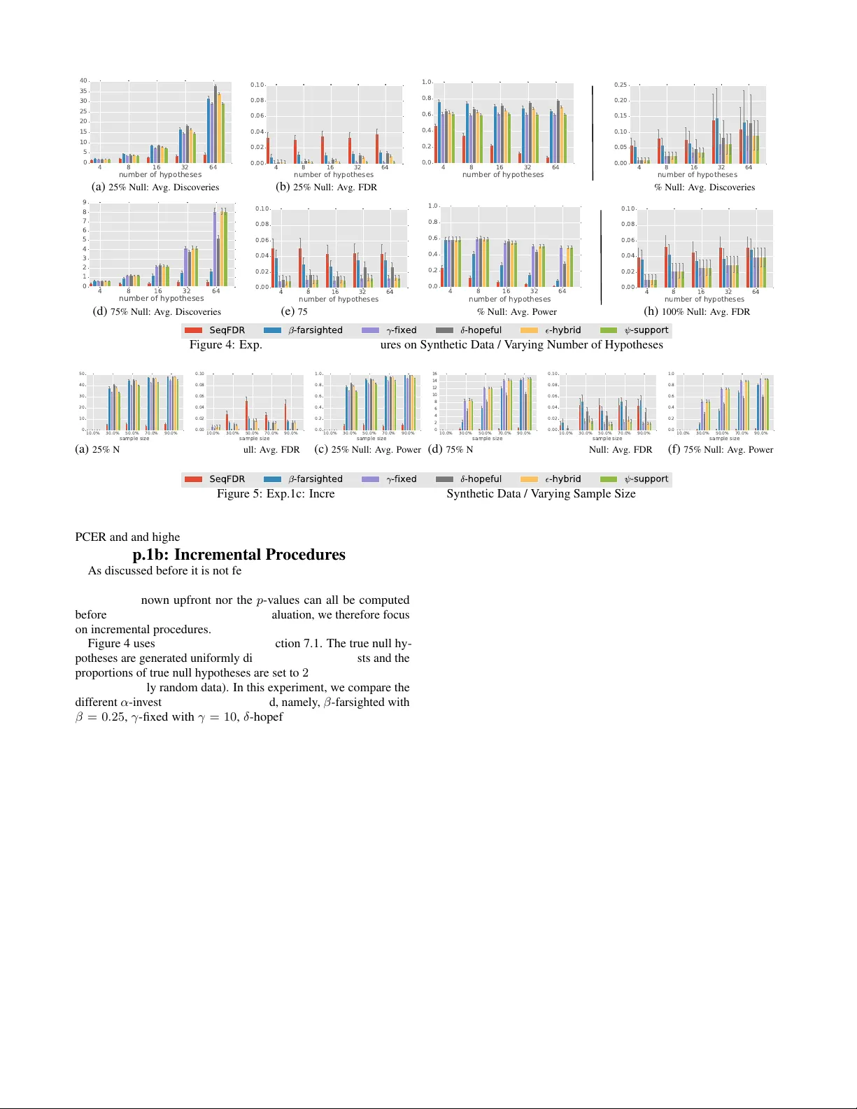
Contr olling F alse Disco veries During Interactive Data Exploration Zheguang Zhao Lorenzo De Stef ani Eman uel Zgraggen Carsten Binnig Eli Upf al Tim Kraska Depar tment of Computer Science, Bro wn University {ﬁrstname_lastname}@brown.edu ABSTRA CT Recent tools for interacti ve data exploration signiﬁcantly increase the chance that users make false disco veries. The crux is that these tools implicitly allo w the user to test a large body of different hy- potheses with just a fe w clicks thus incurring in the issue commonly known in statistics as the “ multiple hypothesis testing err or ”. In this paper , we propose solutions to integrate multiple hypothesis testing control into interactiv e data exploration tools. A key insight is that existing methods for controlling the f alse discov ery rate (such as FDR) are not directly applicable for interacti ve data e xploration. W e therefore discuss a set of new control procedures that are better suited and integrated them in our system called A W A R E . By means of extensi ve e xperiments using both real-world and synthetic data sets we demonstrate how A W A R E can help experts and novice users alike to ef ﬁciently control false discov eries. 1 Introduction “Beer is good for you: study ﬁnds that suds contain anti-viral powers” [DailyNews 10/12]. “Secret to W inning a Nobel Prize? Eat More Chocolate” [T ime, 10/12]. “Scientists ﬁnd the secret of longer life for men (the bad news: Castration is the ke y)” [Daily Mail UK, 09/12]. “ A new study sho ws that drinking a glass of wine is just as good as spending an hour at the gym” [Fox Ne ws, 02/15]. There has been an explosion of data-dri ven discov eries like the ones mentioned abov e. While several of these are legitimate, there is an increasing concern that a large amount of current published research ﬁndings are false [19]. The reasons behind this trend are manifold. In this paper we make the case that the rise of interactive data exploration (IDE) tools has the potential to worsen this situation further . Commercial tools like T ableau or research prototypes like V izdom [9], Dice [22] or imMens [26], aim to enable domain ex- perts and novice users alike to discov er complex correlations and to test hypotheses and dif ferences between v arious populations in an entirely visual manner with just a fe w clicks; unfortunately , often ig- noring e ven the most basic statistical rules. W e recently performed a small user study and asked people to e xplore census data using such an interactiv e data exploration tool. Within minutes, all participants were able to extract multiple insights, such as “ people with a Ph.D. earn mor e than people with a lower educational de gr ee ”. At the same time, almost none of the participants used a statistical method to test whether the difference the visually observed visually from the histogram is actually meaningful. Further, most users including experts with statistical training, did not consider that this type of ex- ploration, that consists of repeated attempts to ﬁnd interesting facts, increases the chance to observ e seemingly signiﬁcant correlations by chance. This problem is well known in the statistics community and referred to as the “ multiple testing problem ” or “ multiple hypothesis err or ” and it denotes the fact the more tests an analysts performs, the higher is the chance that a discov ery is observed by chance. Let us assume an analyst tests 100 potential correlations, 10 of them being true, and she wants to limit the chance of a false disco very to 5% (i.e., the family-wise error rate should be p = 0 . 05 ). Assume further that our test has a statistical power (i.e, the likelihood to discover a real correlation) of 0.8; all very common values for a statistical testing. With this setting, the user will ﬁnd ≈ 13 correlations of which 5 ( ≈ 40 %) are “bogus”. The analyst should use a multiple hypothesis test correction method, such as the Bonferroni correction [6]. Howe ver , Bonferroni correction signiﬁcantly decreases the power of ev ery test and with it the chance of ﬁnding a true insight. This is especially true in the case of interacti ve data exploration, where the number of tests is not known upfront and incremental versions of Bonferroni correction need to be applied which w ould ev en further decrease the power of the tests. Another interesting question concerns what should be considered as a hypothesis test when users interactively explore data. For example, if a user sees a visualization, which sho ws no dif ference in salaries between men and w omen based on their education, b ut later on decides based on that insight to look at salary dif ferences between married men and women. Should we still account for that? The answer in most cases will be “yes” as the analyst probably implicitly made a conclusion based on that visualization, which then in turn triggered her next exploration step. Howev er , if she considers this visualization just as a descriptive statistic of ho w the data looks like, and makes no inference based on it (i.e. it did not inﬂuence the decision process of what to look at ne xt), then it should not be considered as a hypothesis. The difference is subtle and usually very hard to understand for non-e xpert users, while it might hav e a profound impact on the number of false discov eries a user makes. Finally , in the context of data exploration there has been recent work on automatically recommending visualization [36, 23, 37] or correlations [8]. These systems yet again increase the chance of false discoveries since the y automatically test all (or at least a large fraction) of possible combinations of features until something interesting shows up without considering the multiple hypothesis testing problem. In this paper , we make a ﬁrst step to wards integrating automatic multiple hypothesis testing control into an interacti ve data explo- ration tool. W e propose a potential user interface and a meaningful default hypothesis (i.e., the null hypothesis ), which allows us to achiev e control of the ratio of false discov eries for ev ery user inter- action. Speciﬁcally , we propose to consider ev ery visualization as a hypothesis unless the user speciﬁes otherwise. W e further discuss control procedures based on the family-wise error and discuss why they are too pessimistic for interactiv e data exploration tools and why the more modern criteria of controlling the false disco very rate (FDR) is better suited for large scale data exploration. The chal- lenge of FDR, howe ver , is, that the standard techniques, such as the Benjamini-Hochberg procedure are not incremental and require to test all the hypotheses, before determining which hypotheses are rejected. This clearly constitutes a problem in the data e xploration setting where users make discoveries incrementally . The recent α -in vesting technique [14] proposes an incremental procedure to control a variation of FDR, called marginal FDR (mFDR), which howe ver relies on the user having a deep understanding of how valuable each individual test is supposed to be. Again a contradic- tion to data exploration, where the user only o ver time gains a feel about the importance of certain questions. W e therefore propose new strategies based on the α -in vesting procedure [14], which are particular tailored to wards interactiv e data exploration tools. W e implement these ideas in a system called A W A R E and we show ho w this system can help experts and no vice users alike to control f alse discov eries through extensi ve e xperiments on both real-world and synthetic data and workloads. The main contributions can be summarized as follo ws: • W e propose A W A R E , a nov el system which automatically tracks hypotheses during data exploration; • W e discuss se veral multiple hypothesis testing control meth- ods and how well the y work for data exploration; • Based on the previous discussion, we dev elop new α -in vesting rules to control a variant of the false discovery rate (FDR), called marginal FDR (mFDR); • W e e valuate our system using synthetic and real-world datasets and show that our methods indeed achieve control of the number of false discoveries when using an interactiv e data exploration system. The paper is structured as follows: in Section 2 we discuss, by means of an example, why some visualizations should be considered hypothesis tests and what are the main challenges encountered when testing hypotheses for the IDE setting. In Section 3 we present A W A R E ’ s user interface and discuss how to automatically track hypotheses and how to integrate the user feedback into tracking the hypothesis. In Section 4 we discuss multiple hypothesis testing techniques known in literature and sho w how well they ﬁt in the IDE setting. In Section 5 we then propose ne w multiple hypothesis testing procedures for IDE based on the α -in vesting procedure. Afterwards, in Section 7 we present the result of our experimental ev aluation using both real-world and synthetic data. Finally , in Section 8 and 9 we discuss related work and present our conclusions. 2 A Motivational Example T o moti vate the v arious aspects for multi-hypothesis control dur- ing data exploration we outline a potential scenario that is inspired by V izdom [9]. Similar workﬂows ho wev er can be achie ved with other systems like T ableau, imMens [26] or Dice [22]. Let us assume that Eve is a researcher at a non-proﬁt organiza- tion and is working on a project relev ant to a speciﬁc country . She just obtained a ne w dataset containing census information and is now interested in getting an ov erview of this data as well as ex- tracting new insights. She starts off by considering the “ gender ” attribute and observes that the dataset contains the same number of records for men and women (Figure 1 A). She then moves to a second visualization, displaying the distrib ution of people who earn above or below $50k a year . Eve links the tw o charts so that selections in the “ salary ” visualization now ﬁlter the “ gender ” vi- sualization. She notices that by selecting the salaries above $50k, the distribution of “ gender ” is skewed to wards men, suggesting that men have higher salaries than women (B). After creating a third visualization for “ gender ”, selecting the records corresponding to records with salary lower than $50k (dashed line indicates inv ersion of selection), she conﬁrms her ﬁnding “ W omen in this country ar e pr edominately earning less than $50k ” (C). Ev e now wants to un- derstand what else inﬂuences a persons yearly salary and creates a chain of visualizations that selects people who ha ve PhD de grees and are not married (D). Extending this chain using the “ salary ” attribute appears to suggest that this sub-population contains a lot of high-earners (E). By selecting the high-earners and extending the chain with two “ ag e ” visualizations allows her to compare the age distribution of unmarried PhDs earning more than $50k to those making less than $50k. In order to verify that the observed visual difference is actually statistically signiﬁcant she performs a t-test by dragging the two charts close to each other (F). While the example workﬂow contains only one hypothesis test explicitly initiated by the user , we ar gue that without accounting for other implicit hypothesis tests there is a signiﬁcantly increase of risk that the users may observe false discoveries during similar scenarios of data exploration. This opens up ne w important questions: why and when should visualizations be considered statistical hypothesis tests? How should these tests be formulated? 2.1 Hypothesis T esting In this paper , we focus on the widely used frequentist inference approach and its p -value outcome. In order to determine whether there is a correlation between two observed phenomena formalized in a “ resear ch hypothesis ” H that is actually statistical relev ant (i.e., not product of noise in the data) we analyze its corresponding “ null hypothesis ” H which refers to a general statement or default position according to which there is no relationship between two measured phenomena. Giv en this relationship between H and H , the research hypothesis H is also commonly referred as “ alternative hypothesis ”. The testing pr ocedur e will then determine whether to accept (resp., r eject ) a null hypothesis H which in turn corresponds to rejecting (resp., accepting) the corresponding alternative hypothesis (or r esear ch hypothesis ) H . In order to do so the p -value of the null hypothesis H is ev aluated. The p -value is used in the context of null hypothesis testing in order to quantify the idea of statistical signiﬁcance of evidence and it denotes the probability of obtaining an outcome at least as extreme as the one that w as actually observed in the data, under the assumption that H is true. Depending on the context, the p -value of H is ev aluated using the appropriate statistical test (e.g., the t-test or the X 2 -test ). If the p -value p associated to the null hypothesis H is less than or equal to the signiﬁcance level α chosen by the testing procedure (commonly 0 . 05 or 0 . 01 ), the test suggests that the observed data is inconsistent with the null hypothesis, so the null hypothesis must be rejected.This procedure guarantees for a single test, that the probability of a “ false discovery ” (also known as “ false positive ” or “ T ype I err or ”) – wrongly rejecting the null hypothesis of no ef fect – is at most α . This does not imply that the alternati ve hypothesis is true; it just states that the observed data has the likelihood of p ≤ α under the assumption that the null hypothesis is true. The statistical power or sensitivity of a binary hypothesis test is the probability that the test correctly rejects the null hypothesis H when the alternativ e hypothesis H is true. While the frequentist approach to hypothesis test has been crit- icized [20, 28] and there has been a lot of work in developing alternativ e approaches, such as Bayesian tests [5], it is still widely used in practice and we consider it a good ﬁrst choice to build a system which automatically controls the multiple hypotheses error as they hav e two adv antages: (1) Novice users are more likely to hav e experience with standard hypothesis testing than the more de- manding Bayesian testing paradigm. (2) The frequentist inference approach does not require to set a hard-to-determine prior as it is gen der cou nt M ale Fema le Othe r A salary ove r 5 0k cou nt T rue False gen der cou nt M ale Fema le Othe r gen der cou nt M ale Othe r salary ove r 5 0k cou nt T rue False gen der cou nt M ale Fema le Othe r B C edu cati on cou nt HS Bache l or M aste r PhD marit al sta tus cou nt M arrie d N eve r M arrie d N ot M arrie d Wido wed Fema le salary ove r 5 0k cou nt T rue False edu cati on cou nt HS Bache l or M aste r PhD marit al sta tus cou nt M arrie d N eve r M arrie d N ot M arrie d Wido wed age cou nt 10 20 3 0 5 0 60 70 4 0 90 8 0 age cou nt 10 20 3 0 5 0 60 70 4 0 90 8 0 0 . 011 p t-test D E F salary ove r 5 0k cou nt T rue False edu cati on cou nt HS Bache l or M aste r PhD marit al sta tus cou nt M arrie d N eve r M arrie d N ot M arrie d Wido wed Figure 1: An example Interacti ve Data Exploration Session the case with Bayesian tests. 2.2 V isualizations as Hypotheses A visualization per -se sho ws a descriptiv e statistic (e.g., the count of women or the count of men) of the dataset and is not a hypothesis. It is reasonable to assume that in step A of Figure 1 the user just looks at the gender distrib ution and simply ackno wledges that the census surveys roughly the same amount of women and men. How- ev er , it becomes an hypothesis test, if the user expected something else and dra ws a conclusion/inference based on the visualization. For example, if the user somehow assumed that there should be more men than women in the data and therefore considering the fact that there is an equal amount as an insight. The notion of a visualization being considered as a hypothesis becomes ev en clearer in step (B) and (C) of the example work-ﬂow . When looking at the visualization in (B) in isolation, it just depicts a descriptiv e statistic. Indeed, if the user would just take it as such and not make any inference about it and/or base further exploration on an insight extracted from this visualisation, then it would not be considered an hypothesis. W e argue howe ver that the opposite is true more often than not. First, our analytical reasoning and sense-making process is inherently non-linear [29, 33]. Our future actions are inﬂuenced by new kno wledge we discov ered in previous observ ations. Second, while susceptible to certain types of biases [11], the human visual system is highly optimized at picking up differences in visual sig- nals and at detecting patterns [7]. An average user is very likely drawn to the changes between the gender distribution of step (A) and step (B) and might therefore infer that women earn less than men and potentially ﬂag this as an interesting insight that deserves more in vestigation. This is illustrated in step (C) where the user no w further drills down and visually compares the distribution of gender ﬁltered by salary . W e qualitatively conﬁrmed this notion through a formati ve user study where we manually coded user -reported in- sights, following a think-aloud protocol similar to the one proposed in [16]. In this study we observed that users tend to pick up on ev en slight differences in visualizations and reg ard them as insights and users predominantly base future exploration paths on pre viously inferred insights. W e conclude two things: (1) most of the time users indeed treat visualizations as hypotheses, though there are exceptions, and (2) they often (wrongly) assume that what the y see is statistical signiﬁ- cant. The latter is particularly true if the users do not carefully check the axis on the actual count. For example, if a user starts to analyze the outliers of a billion record dataset and makes the conclusion that mainly uneducated whites are causing the outliers, the dataset she is referring to might be comparable small and the chance of randomness might be much higher . The same argument also holds against the critic, that with enough data observing dif ferences by chance are much less likely , which is true. As part of visual data exploration tools, users often explore sub-populations, and while the original dataset might be large, the sub-populati on might be small. Thus, we argue that e very visualization as part of a interacti ve data exploration tool should be treated as a hypothesis and that users should be informed about the signiﬁcance of the insights they gain from the visualization. At the same time, a user should hav e the choice to declare a visualization as just descriptiv e. 2.3 Heuristics f or V isualization Hypotheses A core question remains: what should the hypothesis for a visu- alization be. Ideally , users would tell the system e very single time what they are thinking so that the hypothesis is adjusted based on their assumed insight(s) they gain from the visualization. Ho wev er , this is disruptiv e to any interactiv e data exploration session. W e rather argue that the system should use a good default hypothesis, the user can modify (or e ven delete) if she so desires. For the purpose of this work, we mainly focus on histograms as shown in Figure 1 and acknowledge that there exist man y other visualizations, which we consider as future work. W e deri ved the follo wing heuristics from two separate user studies where we observ ed over 50 participants using a IDE tool to explore v arious datasets. 1. Every visualization without any ﬁlter conditions is not a hy- pothesis (e.g., step A in Figur e 1) unless the user makes it one. This is reasonable, as users usually ﬁrst gain a general high-lev el impression of the data. Furthermore, in order to make it an hypothesis, the user would need to provide some prior kno wledge/expectation, for example as discussed before, that he expected more men than women in the dataset. 2. Every visualization with a ﬁlter condition is a hypothesis with the null-hypothesis that the ﬁlter condition makes no differ ence compared to the distribution of the whole dataset . For example, in step B of Figure 1 the null hypothesis for the distribution of men vs. women given the high salary class of ov er $50 k would be that there is no dif ference compared to the equal distribution of men vs. women over the entire dataset (the visualization in step A). This is again a reasonable assumption as the distrib ution of an attribute gi ven others is only interesting, if it shows some dif ferent effect compared to looking at the whole dataset. 3. If two visualization with the same but some ne gated ﬁlter conditions are put next to each other , it is a test with the null-hypothesis that there is no differ ence between the two visualized distributions, which supersedes the pr evious hy- pothesis. This is the case in step C: gi ven that the user looks explicitly at the distribution of males vs females giv en a salary ov er and under $50 k is a strong hint from the user , that he wants to compare these two distrib utions. As with e very heuristic it is important to note, that the heuristic can be wrong. Therefore it is extremely important to allow the user to overwrite the default hypothesis as well as delete default hypothesis if one really just acted as a descriptive statistic or was just generated as part to a bigger hypothesis test. Furthermore, there exist of course other potential null-hypothesis. For example, in our workﬂo w we assume by default that the user aims to compare distributions, which requires a χ 2 -test. Howe ver , maybe in some scenarios comparing the means (i.e., a t-test) might be more appro- priate as the default test. Y et, studying in detail what a good default null-hypothesis is dependent on the data properties and domain, is beyond the scope of this paper . 2.4 Heuristics A pplied to the Example For our example in Figure 1 the resulting hypothesis could be as follo ws: Step A is not an hypothesis based on rule 1 as it just visualizes the distribution of a single attribute over the whole dataset. Step B is the hypothesis m 1 if the distribution of gender is different giv en a salary ov er $50 k . Step C supersedes the pre vious h ypothesis and replaces it with an hypothesis m 0 1 if the gender distribution between a salary over and under $50 k is dif ferent, which is a sightly different question. Step D creates a hypothesis m 2 if the marital status for people with PhDs is different compared to the entire dataset, whereas step-E generates a hypothesis m 3 if there is a different salary distribution given not married people with a PhD. By studying the age distribution in step F the system ﬁrst generated a default hypothesis m 4 that the distribution of the ages is dif ferent giv en a PhD and being not married for different salary classes. Howe ver , the user overwrites immediately the default hypothesis with an hypothesis m 0 4 about the av erage age. Furthermore, as the previous visualizations in step D and E might just have been stepping stones to wards creating m 4 the user might or might not delete hypothesis m 2 and m 3 . Howe ver , if the insights our user gained from vie wing the marital status, etc., inﬂuenced her to look at the age distribution, she might w ant to keep them as hypothesis. Clearly this is only a v ery small example, b ut it already demon- strates the general issues. Not ev ery insight the user gains (e.g., the insight that women earn less) is explicitly expressed as a test. At the same time, as more the user “surfs” around the higher the chance that she ﬁnds something which looks interesting, but just appears because of chance. In the example abov e, by the time the user actually performs its ﬁrst test (step F), she implicitly already tested at least one other hypothesis and potentially even four others. Assuming a targeted p -value of α = 0 . 05 , the chance of a false discov ery therefore increased to 1 − (1 − α ) 2 = 0 . 098 for two hypothesis and up to 1 − (1 − α ) 4 = 0 . 185 for four hypothesis. While the question of what should count as an hypothesis is highly dependent on the user and can nev er be fully controlled by any system, we can howe ver , enable the system to make good sugges- tions and help users to track the risk of making false discoveries by chance. Furthermore, this short workﬂow also demonstrates that hypotheses are b uilt by adding but also by remo ving attributes. As we will discuss later, there exist no good method so far to control the risk of making f alse discov eries for incremental sessions lik e the ones created by interacti ve data e xploration systems. W e therefore dev elop new methods especially for interactiv e data exploration in Section 5. Finally , it should be noted, that the same problems also exist with exploratory analysis using SQL or other tools. Howe ver , we argue that the situation is becoming worse by the up-rise of visual exploration tools, like T ableau, which are often used by novice users, who not necessarily reﬂect enough on their exploration path after they found something interesting. 3 The A W A R E User Interface As argued in the previous section, user feedback is essential in determining, tracking and controlling the right hypothesis during the data exploration process. With A W A R E we created a system that applies our heuristic automatically to all visualizations. W e designed A W A R E ’ s user interface with a fe w goals in mind. First, the user should be able to see the hypotheses the system assumed so far , their p -values , effect sizes and if they are considered signiﬁcant and should be able to change, add or delete hypotheses at any gi ven stage of the e xploration. Second, hypotheses rejection decisions should ne ver change based on future user actions unless the user explicitly asks for it. W e therefore require an incremental procedure to control the multiple hypothesis risk that does not change its rejection decisions e ven if more hypothesis tests are executed. For e xample, the system should not state that their is a signiﬁcant age difference for not married highly educated people, and then later on rev oke its assessment just because the user did more tests. More formally , if the system de- termined which hypotheses m 1 ...m n are signiﬁcant (i.e., it rejects the null) or not and the user changes the last hypothesis or adds an hypothesis m n +1 , which should be the most common cases, the signiﬁcance of hypotheses m 1 ..m n should not change. Howev er , if the user might change, delete, or add hypothesis k ∈ 1 , .., n , de- pending on the used procedure we might allow that the signiﬁcance of hypotheses m k +1 to m n might hav e to change as well. Third, individual hypothesis descriptions should be augmented with information about how much data n H 1 the user has to add, under the assumption that the new data will follow the current observed distrib ution of the data, to make an hypothesis signiﬁcant. While sounding counter-intuiti ve, as one might (wrongly) imply , it is possible to make any hypothesis true by adding more data, calculating this value is in some ﬁelds already common practice. For e xample, in genetics scientist often search (automatically) for correlations between genes and high-le vel ef fects (like cancer). If such a correlation is found, often because of the multiple hypothesis error the chance of a true discov ery is tiny (i.e., the p -value is too high). In that case the scientist works backwards and estimates how much more genes she has to to sequence in order to make the hypothesis relev ant, expecting that the new data (e.g., gene sequences) follow the same distribution of the data the scientist already has. Howe ver , if the effect was just produced by chance, the ne w data will be more similar to the distribution of the null- hypothesis and the null will not be rejected. The required v alue is generally easy to calculate or approximate, and are highly valuable for the end-user . A small v alue for n H 1 in relation to the number of totally tested hypotheses might be an indication that the power (i.e., the chance to accept a true alternati ve hypothesis) of the test was not suf ﬁciently large. And ﬁnally , users should be able to bookmark important hypothe- ses. Our system uses default hypothesis throughout the exploration and the user might ﬁnd it too cumbersome to correct everyone for his real intentions, there might be more hypotheses generated than the user intended to test. Even if all hypotheses are what the user was considering, some of them might be more important to her than others; the hypotheses the user would like to include in a presen- tation or show to her boss. A key key question becomes, what is the expected number of false discov eries among those important alph a 2. 5% 5% salary | edu cat ion <> salary H 1 0 . 02 7 t-test salary | edu cat ion = sala ry H 0 coh en' s d 0 . 5 H 1 0 . 001 t-test H 0 coh en' s d 0 . 8 age | {ch ain } <> ag e | {c hai n-1} H 1 0 . 011 t-test age | {ch ain } = a ge | { cha in-1} H 0 coh en' s d 0 . 5 gen der | m arita l = g end er H 1 0 . 621 chi squa re gen der | m arita l = g end er H 0 coh en' s d 0 . 01 A B C D E salary | {ch ain -1} <> sal ary salary | {ch ain -1} = sa lary Figure 2: The A W A R E User Interface discov eries? Figure 2 shows the current interface design of A W A R E with a risk controller , which incorporates the above ideas, running on a tablet. The user interface features an unbounded 2D can v as where chains of visualizations (such as the one shown in Figure 1) can be laid out in a free form fashion. A “risk-gauge” on the right-hand side of the display (Figure 2 (A)) serves two purposes: it gives users a summary of the underlying procedure (e.g., the budget for the false discovery rate set to 5% with current remaining wealth of 2.5%; both explained in the next two sections) and it provides access to a scrollable list of all the hypothesis tests (implicit and explicit) that have been execute so far . Each list entry displays details about one test and its results. T extual labels describe the null- and alternati ve-hypothesis and color coded p -values indicate if the null-hypothesis was rejected or accepted (green for rejected, red for accepted). Furthermore, it visualizes the distribution of null-hypothesis and alternati ve hypothesis and sho ws its difference, included an indication of its color coded ef fect size (D). T ap gestures on a speciﬁc item allow users to change things like the default hypothesis or the type of test. Additionally other information such as an estimation of the size of an additional data n H 1 that could make the observation signiﬁcant can be displayed in each item. In the example this information is encoded through a set of small squares (B, C) where each square indicates the amount of data that is in the corresponding distribution. In (B) the ﬁv e red squares tells us that we need 5x the amount of data from the null-distribution to ﬂip this test form rejected to accepted or con versely in (C) 11.5x the amount of data from the alternativ e-distribution to rejected this hypothesis. Finally , we allow to mark important hypotheses by tapping the “star” icons (E). 4 Background on Multiple Hypothesis Err or The pre vious section described how we con ve y the multiple hy- pothesis error to the user and ask for user feedback to deriv e the right hypothesis. In this section we describe dif ferent alternativ es to calculate the potential false discov ery error and discuss they appro- priateness for the IDE setting. The notation used in the rest of the paper is summarized in Appendix A. W e consider a setting, in which we ev aluate the statistical rel- ev ance of hypotheses from a set H = H 1 , H 2 , . . . , H m , created incrementally by an IDE system in a streaming fashion. In order to verify whether any such hypothesis H j is in fact statistically relev ant we consider its corresponding null hypothesis H j . Using the appropriate statistical test (e.g., the t-test or the X 2 -test ) the p -value of H j ev aluated and based on it the testing procedure deter- mine whether to accept (resp., r eject ) a null hypothesis H j which in turn corresponds to rejecting (resp., accepting) the corresponding alternative hypothesis (or r esear ch hypothesis ) H | . The hypothesis according to which all null hypotheses are true is referred as the “ complete ” or “ global ” null hypothesis. The set of null hypotheses rejected by a statistical test are called “ discoveries ”and are denoted as R . Among these we distinguish the set of true discoveries S , and the set of false discoveries or false positives V ; i.e., | V | + | S | = | R | False discov eries are commonly referred also as T ype 1 errors. Null hypotheses in S are false null hypotheses , while null hypotheses in V are true null hypotheses . 4.1 Hold-Out Dataset A possible method to deal with the multiple hypothesis error is to split the dataset D into a exploration D 1 and a validation D 2 dataset [38]. D 1 is then used for the data exploration process, whereas the validation dataset is used to re-test all hypotheses in order to validate the results of the ﬁrst phase. In the following we will pro vide some examples which will clarify ho w , albeit useful, a hold-out dataset does not solve the multiple hypothesis testing problem. Let us consider a null hypothesis H , and let p D denote its associ- ated p -value when H is ev aluated with respect of the entire dataset D . Lets assume we perform a test with signiﬁcance-le vel α . In this case the probability of wrongly rejecting H is at most α Suppose now that we randomly split the dataset into two datasets D 1 and D 2 . For the same null hypothesis H we e valuate the p -values p D 1 and p D 2 each obtained by e valuating H on D 1 or D 2 respectiv ely . W e then run a a test with signiﬁcance-level α (like the one discussed abov e) for each of the datasets. W e then decide to reject H if it has been rejected by both the testing procedures operating on the datasets D 1 or D 2 . If both procedures operating on D 1 and D 2 hav e signiﬁcance-lev el α , then the probability that the ov erall procedure ends up rejecting H is at most α 2 . For the common v alue of α = 0 . 05 , the chance of a T ype I error is thus reduced to 0 . 0025 , which is good news. Rather than fully handling the multiple hypothesis problem, what we ha ve achie ved trough this procedure is ho wev er just the lowering of the threshold for rejecting the null hypothesis (i.e., the signiﬁcance le vel of the test). This fact appears clearly in the follo wing scenario. Suppose that the user wants to ev aluate multiple hypotheses (e.g., 25) rather than just one. Assuming that these hypotheses, and their p -values are independent, the probability of observing at least one erroneous rejection using the test technique based on the use of the holdout dataset would be: p f = 1 − (1 − p D ) 25 ≈ 0 . 06 , which is higher than the desired α signiﬁcance lev el. Albeit the lowering of the achie ved reduction of the signiﬁcance lev el is indeed useful for reducing the chance of T ype I errors, it comes at the cost of a signiﬁcant reduction of the power of the testing procedure. Let us consider the following e xample scenario in which we aim to compare the means M 1 and M 2 of two samples one drawn from a population with expected value µ 1 = 0 and the other from a population with µ 2 = 1 , both having a standard de viation of σ = 4 . In order to determinate weather the observed difference between M 1 an M 2 is actually statistically signiﬁcant, we test the null-hypothesis “ ther e is no signiﬁcant differ ence between µ 1 and µ 2 ” using the one-sided t-test and a sample composed by 500 records from each population. Giv en the properties of the t-test (see [13]), the statistical power of our test would be 0 . 99 , and the probability of erroneously accepting the null hypothesis would be at most 0 . 01 . Suppose no w that we divide the dataset into a dataset for e xplo- ration and one for validation each composed by 250 records. The statistical power for each of the individual t-test executed on the two dataset is now lo wered to 0 . 87 , due to the reduction of the data being used. Further , recall that the procedure based on the holdout set rejects a null hypothesis only if said hypothesis is rejected by both sub-tests. This implies that the actual overall power of the testing procedure is 0 . 87 · 0 . 87 ≈ 0 . 76 , which is signiﬁcantly lower than the 0 . 99 achiev ed by the test which uses the entire data. In general, approaches based on hold-out datasets are considered inferior compared to testing o ver the entire dataset. In some sce- narios, like building machine learning models, hold-out datasets might e ven be the only possibility to test a model or tune parameters. In those cases, a hold-out approach (like k-fold cross-validation) should be considered as test and should be controlled for the multiple hypothesis error as recent work suggests [10, 24, 30]. It is howe ver important to remark that in our work we aim to predict guarantees on the statistical signiﬁcance of the statistical predictors which are instead not achiev able using prediction-dri ven approaches such as cross-validation. 4.2 F amily-Wise Err or Rate (FWER) T raditionally , frequentist methods for multiple comparisons test- ing focus on correcting for modest numbers of comparisons. A natural generalization of the signiﬁcance le vel to multiple hypothe- sis testing is the F amily W ise Err or Rate , which is the probability of incurring at least one T ype I error in any of the individual tests. The FWER is the probability of making at least one type I error in the family: F W E R = Pr( V ≥ 1) = 1 − Pr( V = 0) (1) By assuring that F W E R ≤ α , that is the FWER is contr olled at level α , we hav e that the probability of e ven one T ype I error in ev aluating a family of hypotheses is at most α . W e say that a procedure controls the FWER in the weak sense , if the FWER control at le vel α is guaranteed only when all null hypotheses are true (i.e. when the complete null hypothesis is true). W e say that a procedure controls the FWER in the str ong sense , if the FWER control at lev el α is guaranteed for any conﬁguration of true and non-true null hypotheses (including the global null hypothesis). Bonferroni Correction: The Bonferroni correction is the sim- plest statistical procedure for multiple hypothesis testing [6]. Let α be the critical threshold for the test. The v alue of α is usually selected at 0 . 01 or 0 . 05 . Let p i the p -value statistic associated with the null hypothesis H i . When testing m distinct null hypotheses using the Bonferroni correction, a null hypothesis H i is rejected if p i ≤ α/m . The Bonferroni procedure thus achiev es control of the FWER at level α . Unfortunately , the Bonferroni correction can not be applied in our setting as it requires kno wledge of the total number of hypotheses being considered. An alternativ e approach is to use a variation of the Bonferroni correction, according to which the j -th null hypothesis H j is rejected if p j ≤ α · 2 − j . It is possible to show that this procedure indeed controls FWER at le vel α as j → ∞ and does not need explicit kno wledge of m . Howe ver the acceptance threshold decreases exponentially with respect to the number of hypotheses, thus resulting in a high number of false neg ativ es. The main common issue with all FWER techniques is that the power of the test signiﬁcantly decreases as m increases due to the corresponding decrease in the acceptance threshold ( α/m in the original Bonferroni or α/ 2 i in the sequential variant). While some alternati ve testing procedures such as those of V ˇ idák [34], Holm [18], Hochberg [17], and Simes [35] of fer more power while controlling FWER, the achiev ed improvements are generally minor . A review of sev eral of these techniques is provided by Shaffer in [32]. 4.3 F alse Discovery Rate (FDR) In [2] Benjamini and Hochberg proposed the notion of F alse Discovery Rate (FDR) as a less conservati ve approach to control errors in multiple tests which achie ve a substantial increase in the power of the testing procedure. FDR-controlling procedures are designed to control the expected ratio Q = V /R of false discov eries among all discoveries returned by a procedure. In particular , the FDR of a statistical procedure is deﬁned as: F D R = E [ Q ] = E  V R | R > 0  P ( R > 0) . (2) Howe ver , if we deﬁne FDR to be zero when R = 0 , we can simplify 2 to: F D R = E  V R  (3) W e say that a testing procedure controls FDR at level α if we hav e F DR ≤ α . Designing a statistical test that controls for FDR is not simple, as the FDR is a function of two random variables that depend both on the set of null hypotheses and the set of alter- nativ e hypotheses. The standard technique to control the FDR is the Benjamini-Hochber g procedur e (BH), which operates as follo ws: let p 1 ≤ p 2 ≤ . . . ≤ p m be the sorted order of the the p -values for the m tested null hypotheses. T o control FDR at lev el α (for independent null p -values) determine the maximum k for which p k ≤ k m · α , and reject the null hypotheses corresponding to the p -values p 1 , p 2 , . . . , p k . Interestingly , under the complete null hypothesis, controlling the FDR at lev el α guarantees also “ weak control ” ov er the FWER F W E R = P ( V ≥ 1) = E  V R  = FDR ≤ α . This follows from the fact that the ev ent of rejecting at least one true null hypoth- esis V ≥ 1 is exactly the ev ent V /R = 1 , and the event V = 0 is exactly the e vent V /R = 0 (recall V /R = 0 when V = R = 0 ). This makes the FDR relati vely easy to explain to the user as under complete random data, the chance of one or more false disco veries is at most α as in FWER. Ho wev er , FDR does not howe ver ensure control of the FWER if there are some true discov eries to be made (i.e., it does not ensure “ str ong contr ol ” of the FWER). Because of its increased power , FDR appears to be a better candi- date than FWER in the conte xt interactiv e data exploration, where usually a larger number of hypotheses are to be considered. Unfor- tunately , both the original Benjamini-Hochber g pr ocedure and its variation for dealing with dependent hypotheses [3] are not incre- mental as they require knowledge of the total number of hypotheses being tested (similar to what was discussed for Bonferroni) and of the sorted list of all the p -values corresponding to each null hypothesis being e valuated. An adaptation of the FDR technique to a setting for which an unspeciﬁed number of null hypotheses are observ ed incrementally was recently discussed in [15]. The main idea behind the Sequen- tial FDR procedure is to con vert the arbitrary sequence of p -values corresponding to the null hypotheses observed on the stream of hy- potheses into an ordered sequence akin to the one generated by the classical Benjamini-Hochberg procedure. The natural application for this technique is the progressiv e reﬁnement of a model by consid- ering additional features. That is, it starts constructing a model for the data with something kno wn and general. The user then proceeds to reﬁne the model by determining the most signiﬁcant features. One drawback of the Sequential FDR method, is giv en by the fact that the order according to which the hypotheses are observ ed on the stream heavily inﬂuences the outcome of the procedure. For example, if an hypothesis with high p -value is observ ed among the ﬁrst in the stream, this will harm the ability of the procedure of rejecting follo wing null hypotheses, e ven if the y hav e low p -value (see discussion in [15]). This aspect makes Sequential FDR not applicable for data exploration system for which the user is lik ely to explore dif ferent “ avenues ” of discovery rather than focusing on the specialization of a model. 4.4 Other A pproaches Although for most practical applications, FDR controlling pro- cedures constitute the de facto standar d for multiple hypothesis testing [12], many other techniques hav e been presented in the litera- ture. Among them, Bayesian techniques are particularly note worthy . In [5], alternativ e solutions to the multple hypothesis problem com- bining decision theory with Bayesian FDR are discussed. Howe ver , as often the case with Bayesian approaches, the computational cost for these procedures when applied to lar ge datasets are signiﬁcant, and the results are highly dependent on the prior model assumptions. Another approach is correcting for the multiplicity through simu- lations (e.g., the permutation test [31]) that e xperimentally ev aluate the probability of an observ ation in the null distribution. This ap- proach is also not practical in large datasets because of the large number of dif ferent possible observations and the need to e valuate very small p -v alues of each of these distributions [21]. In this paper, we elect to use a family of multiple hypothesis testing procedures know as α -in vesting introduced in [14] and then generalized in [1]. These procedures are especially interesting for the incremental and interactiv e nature of interactiv e data e xploration. The details of α -in vesting and its application to our setting is exten- siv ely discussed in the next section. 5 Interactive Contr ol using α -In vesting One drawback of the Sequential FDR procedure [15] as well as adaptations of FWER controlling techniques to the streaming setting is gi ven by the fact that decisions reg arding the rejection or accep- tance of previously considered null hypotheses could potentially be ov erturned in latter stages due to ne w hypotheses being consid- ered. Although statistically sound, this fact could appear extremely counter intuiti ve and confusing to the user . The only way to adopt the Sequential FDR procedure to data e xploration would be to batch all the hypotheses and only present the ﬁnal decisions afterwards. In that sense Sequential FDR is incremental b ut non-interacti ve in data exploration. In order to have both incremental and interactiv e multiple hy- pothesis error control, we consider a dif ferent approach for multiple hypothesis testing based on the “ α -in vesting ” testing procedure introduced originally introduced by Foster and Stine in [14]. Simi- larly to Sequential-FDR , this procedure does not require explicit knowledge of the total number of hypotheses being tested and can therefore be applied in the hypothesis streaming setting. α -in vesting presents howe ver several crucial differences with respect to both traditional and sequential FDR control procedures. In the following, we ﬁrst introduce the general outline of the procedure as presented in [14] and then discuss sev eral in vesting strategies (called policies) that we have developed for interactiv e data exploration. 5.1 Outline of the Procedur e For α -in vesting , the quantity being controlled is not the clas- sic FDR but rather an alternati ve quantity called “ mar ginal FDR (mFDR) ”: mF D R η ( j ) = E [ V ( j )] E [ R ( j )] + η (4) where j denotes the total number of tests which have been e xecuted, while V ( j ) (resp., R ( j ) ) denote the number of false (resp., total) discov eries obtained using the α -in vesting procedure. In particular , we say that a testing procedure controls mF DR η at lev el α if mF DR η ( j ) ≤ α . The parameter η is introduced in order to weight the impact of cases for which the number of discov eries is limited. Common choices for η are 1 , (1 − α ) , whereas the procedure appears to lose in power for v alues of η close to 0 [14]. Under the complete null hypothesis we ha ve V ( j ) = R ( j ) hence mF DR η ( j ) ≤ α implies that E [ V ( j )] ≤ αη / (1 − α ) . If we chose η = 1 − α then E [ V ( j )] ≤ α , and we can thus conclude that control of the mF DR 1 − α at le vel α implies weak control fo the FWER at le vel α [14]. W e refer the reader to the original paper of Foster and Stine [14] for an extensi ve discussion on the relationship between mF DR and the classic FDR. A generalization of the α - in vesting procedure was later introduced in [1]. The α -in vesting procedure does not in general require any assumption regarding the independence of the hypotheses being tested, although opportune corrections are necessary in order to deal with possible dependencies. In our analysis, we howe ver assume that all the hypotheses and the corresponding p -values are indeed independent. Intuitiv ely the α -in vesting procedure works as follows: With ev ery test j the users sets an α j -value, which has to be below the current wealth, which is in the beginning usually α · (1 − α ) before he performs the test. If the null-hypothesis is accepted ( p j > α j ) the in vested alpha value is lost. T o some degree this is similar to the Bonferroni-correction as one could consider the α j value ev erybody is compared to as α/m . So whenev er a test is performed, the wealth decreases by α/m until the wealth is 0 and the user has to stop exploring. Ho wev er , in contrast to the Bonferroni-correction, with α -in vesting the user can reg ain wealth through a rejected null- hypothesis, which makes the procedure truly incremental as it does no longer depend on the number of anticipated hypotheses m and also more powerful. More formally , we denote as W (0) the initial α -wealth assigned to the testing procedure. If the goal of the testing procedure is to control mF DR η at lev el α , then we shall set W (0) = α · η . Here, η is commonly set to (1 − α ) . W e denote as W ( j ) the amount of “ available α - wealth ” after j tests have being e xecuted. Each time a null hypothesis H j is being tested, it is assigned a budget α j > 0 . Let p j denote the p -value associated with the null hypothesis H j . This hypothesis is rejected if p j ≤ α j . If H j is rejected than the testing procedure obtains a “ r eturn ” on its in vestment ω ≤ α . Instead, if the null hypothesis H j is accepted, α j / (1 − α j ) alpha wealth is deducted from the available α -wealth: W ( t ) − W ( t − 1) = ( ω if p j ≤ α j , − α j 1 − α j if p j > α j (5) The testing procedure halts when the a vailable α -wealth reaches 0 . At that point in time, the user should stop exploring to guarantee that mF DR ≤ α . Obviously again something, which is not desirable as it is hard to conv ey to any user , that he has to stop exploring. W e will discuss this problem and potential solutions in Section 5.8. The budget α j which can be assigned to test must be such that regardless of the outcome of the test, the available α -wealth av ailable after the test is not negativ e W ( j ) ≥ 0 , hence α j ≤ W ( j − 1) / (1 − W ( j − 1)) . Further we impose that α j < 1 . While this constraint was not e xplicated in [14], it is indeed necessary for the correct functioning of the procedure. Setting α j = 1 would lead to the potential deduction of an inﬁnite amount of α -wealth, violating the non neg ativity of W ( j ) . Setting α j > 1 would instead lead to having a positiv e increase of the available α -wealth re gardless of the outcome of the test. In our analysis we will ho wev er assume that all the hypotheses being considered are indeed independent and their associated p -values are independent as well. W e refer as “ α - in vesting rule ” to the polic y according to which av ailable budget has to be assigned to the hypotheses that needs to be tested. Furthermore, in [14] it was shown that any α -in vesting policy for which W (0) = η · α , ω = α , and which obeys the rule in (5), controls the mF D R at level α , for α, η ∈ [0 , 1] . The freedom of assigning to each hypothesis a speciﬁc level of conﬁdence independent of the order, and the possibility of “ r e- in vesting ” the wealth obtained by previous rejection constitute great advantages with respect to the Sequential FDR procedure. 5.2 α -In vesting for Data Exploration While it is relati vely straightforw ard to devise in vesting rules, it is difﬁcult a priori to determinate the “ best way to in vest ” the a vailable alpha -wealth. If α j is picked too small, the statistical power of ev ery test is reduced and the chance is e ven higher too loose the in vested wealth giv en a true alternative hypothesis. If α j is too large, the entire α wealth might be quickly exhausted and the user (in theory) has to stop exploring or re-e valuate all his test (see also Section 5.8). A polic y is most likely to be successful if it can e xploit some knowledge of the testing setting. Another complication is the construction of tests for which one can obtain the needed p -values . T o show that a testing procedure controls mF DR , we require that conditionally on the prior j - 1 outcomes (denoted as R i ), the lev el of the test of H j must not exceed α j : P ( R j = 1 | R j 1 , R j 2 , ..., R 1 ) ≤ α j . (6) This does not ho wev er constitute a problem in our setting as we are assuming all hypotheses and their p -v alue to be independent. While [14] proposed v arious in vesting rules, most of the proposed procedures might test a hypothesis again and o verturn an initial re- jection of a null-hypothesis. Therefore, in the remainder of this section we propose different α -in vesting policies particular for Inter - activ e Data Exploration, which correspond to different e xploration strategies and at exploiting dif ferent possible properties of the data. Howe ver it should be noted, that our ﬁrst procedure, β -farsighted, is a generalization of the “ Best-foot-forwar d policy ” in [14]. For this paper , we consider a setting for which we observe a (potentially inﬁnite) stream of null hypotheses for which at each of the discretized time steps a ne w null hypothesis is observed on the stream. W e denote as H j the hypothesis being considered at the j -th step. W e further assume that said hypotheses are independent. All our policies assign to each hypothesis a strictly positi ve budget α j > 0 as long as any α -wealth is a vailable. If p j ≤ α j , the null hypothesis H j is rejected (i.e., it is considered a disco very). V ice versa, if p j > α j is accepted . The current α -wealth W ( j ) is then updated according to the rule in (5) and because of it controls mF DR at le vel α as shown in [14]. 5.3 β -Farsighted In vesting Rule Like with real in vestment, the question is if one should inv est short or long-term. With β -farsighted we created a policy , which tries to preserve wealth over long exploration sessions. Giv en β ∈ [0 , 1) , we say that a policy is β -farsighted if it ensures that re gardless of the outcome of the j -th test at least a fraction β of the current α -wealth W ( j − 1) is preserved for future tests, that is for j = 1 , 2 , . . . : W ( j ) ≥ β W ( j − 1) , W ( j ) − W ( j − 1) ≥ ( β − 1) W ( j − 1) (7) W e therefore deﬁne the β -farsighted procedure to control mF DR η at lev el α in the procedure for In vesting Rule 1. In vesting Rule 1 β -farsighted 1: W (0) = η α 2: for j = 1 , 2 , ... do 3: α j = min  α, W ( j − 1)(1 − β ) 1+ W ( j − 1)(1 − β )  4: if p ( H j ) < α j then 5: W ( j ) = W ( j − 1) + ω 6: else 7: W ( j ) = W ( j − 1) − α j 1 − α j = β W ( j − 1) 8: end if 9: end for Different choices for the parameter β ∈ [0 , 1) characterize ho w conservati ve the in vesting polic y is. If there is high conﬁdence on the ﬁrst observed hypotheses being true discoveries, small v alues of beta (i.e., 0.25) would be more effecti ve. V ice versa, high values of β (i.e. 0.9) ensure that ev en if the ﬁrst hypotheses are true null, a large part of the α -wealth is preserv ed. W e say that an α in vesting polic y is “ thrifty ” if it ne ver fully com- mits its av ailable α -wealth. The described β -farsighted is indeed thrifty . While the procedure will nev er halt due to the av ailable α -wealth reaching zero, after a long series of acceptance of null hypotheses the a vailable b udget may be reduced so much that it will be effecti vely impossible to reject any more null hypotheses. Although these policies may appear wasteful as there is no re- ward for wealth which has not been inv ested, they are aimed to preserve some of their current budget for future tests in case the hypotheses considered in the beginning of the testing procedure are not particularly trustworthy . This inv esting rule is therefore particular suited for scenarios were the total number of false disco veries in long exploration sessions, potentially across multiple users, should be controlled. 5.4 γ -Fixed In vesting Rule A dif ferent non-thrifty procedure assigns to each hypothesis the same budget α ∗ . In particular, we call γ -ﬁxed a procedure that assigns to each null hypothesis a ﬁxed budget α j equal to a fraction of the initial α -wealth W (0) , that is α ∗ = W (0) / ( W (0) + γ ) , as long as any α -wealth is a vailable. The details of the γ -ﬁxed procedure controlling mF DR η at le vel α can be found in the procedure for In vesting Rule 2. In vesting Rule 2 γ -ﬁxed 1: W (0) = η α 2: α ∗ = W (0) γ + W (0) 3: while W ( j − 1) − α ∗ 1 − α ∗ ≥ 0 , for j = 1 , 2 , . . . do 4: if p ( H j ) < α ∗ then 5: W ( j ) = W ( j − 1) + ω 6: else 7: W ( j ) = W ( j − 1) − α ∗ 1 − α ∗ = W ( j − 1) − W (0) γ 8: end if 9: end while Note that we deﬁne α ∗ as W (0) / ( γ + W (0)) to ensure that the subtraction of the wealth is constantly W (0) /γ . Different choices for the parameter γ characterize how conservati ve the in vesting policy is. If there is high conﬁdence on the ﬁrst observ ed h ypotheses being actual disco veries small values of γ (i.e. 5,10,20) would mak e more sense. V ice v ersa a high value of γ ensures that even if the ﬁrst hypotheses are true null, a large part of the α wealth is preserved. Good choices for that setting would be γ = 50 , 100 . 5.5 δ -Hopeful In vesting Rule In a slight variation of the γ -ﬁxed in vesting rule, we say that a policy is δ -hopeful if the budget is assigned to each hypothesis “ hoping ” that at least one of the ne xt δ hypotheses will be rejected. Each time a null hypothesis is rejected the budget obtained from the rejection is re-inv ested when assigning budget over the next δ null hypotheses. γ -ﬁxed and δ -hopeful operate by spreading the amount of α -wealth ov er a ﬁxed number of hypotheses (either γ or δ ), δ -hopeful is howev er “ less conservative ” than γ -ﬁxed as it always operates by in vesting all currently av ailable α -wealth ov er the next δ hypotheses. So it is a much more optimistic procedure, which works well if most alternative hypotheses are expected to accepted. The details of the δ -ﬁxed procedure controlling mF DR η at lev el α can be found in the procedure for In vesting Rule 3. 5.6  -Hybrid In vesting Rule Because α -in vesting allows contextual information to be incor - porated, the power of the resulting procedure is related to ho w well In vesting Rule 3 δ -hopeful 1: W (0) = η α 2: α ∗ = W (0) δ + W (0) 3: k ∗ = 0 4: while W ( j − 1) − α ∗ 1 − α ∗ ≥ 0 , for j = 1 , 2 , . . . do 5: if p ( H j ) < α ∗ then 6: W ( j ) = W ( j − 1) + ω 7: α ∗ = min  α, W ( j ) δ + W ( j )  8: k ∗ = j 9: else 10: W ( j ) = W ( j − 1) − α ∗ 1 − α ∗ = W ( j − 1) − W ( k ∗ ) α ∗ 11: end if 12: end while the design heuristic ﬁts the actual data exploration scenario. For example, when the data exhibits more randomness, the γ -ﬁxed rule tends to have more power than the δ -hopeful rule. Intuitiv ely , the α -wealth decreases when testing a true null hypothesis, because the expectation of the change of wealth is negati ve when the p -value is uniformly distrib uted on [0 , 1] . Thus the initial α -wealth is on av erage larger than the α -wealth av ailable at subsequent steps. Fur- thermore, since the γ -ﬁxed rule inv ests a constant fraction of the initial wealth, the power tends to be lar ger than δ -hopeful. On the contrary , when the data is less random, the γ -ﬁxed rule becomes less po werful than δ -hopeful rule. The reason is that in this setting more signiﬁcant discoveries tend to keep the subsequent α -wealth high, potentially e ven higher than the initial wealth. W e study this difference in more detail in Section 7. In order to hav e a robust performance in terms of po wer and false discov ery rate, we design  -hybrid in vesting rule that adjust the α j assigned to the various tests based on the estimated data randomness. Our estimation of the randomness of the data is based on the ratio of rejected null hypothesis over a sliding windo w H d constituted by the last d null hypotheses observed on a stream. W e then compare this ration with a “ randomness thr eshold ”  ∈ (0 , 1) and we conclude whether the data exhibits high randomness or not. The procedures is outlined in In vesting Rule 4. In vesting Rule 4  -hybrid 1: W (0) = η α 2: k ∗ = 0 3: H d = [] // Sliding window of size d 4: while W ( j − 1) > 0 , for j = 1 , 2 , . . . do 5: if Rejected( H d ) ≤ | H d |  then 6: α j = W (0) γ + W (0) 7: else 8: α j = min  α, W ( k ∗ ) δ + W ( k ∗ )  9: end if 10: if W ( j − 1) − α j 1 − α j ≥ 0 then 11: if p ( H j ) < α j then 12: W ( j ) = W ( j − 1) + ω 13: k ∗ = j 14: H d [ j ] = R j = 1 15: else 16: W ( j ) = W ( j − 1) − α j 1 − α j 17: H d [ j ] = R j = 0 18: end if 19: end if 20: end while 5.7 In vestment based on Support Population In this section we discuss how to adjust the budget of each hy- pothesis according to the amount of data which is available in order to compute the p -value of that same hypothesis. The main intuition for this procedure is that, as it is most lik ely to observe high p -values for hypotheses which rely on a small number of data points, we should should not in vest as much α -wealth on those hypotheses. In this section we discuss ho w to bias the amount b udget assigned to each hypothesis so that hypotheses with more support data receiv e more “ trust ” (in terms of budget) from the procedure. Let us denote as | n | the total amount of data being used and by | j | the available data for testing the j -th null hypothesis H t . A simple way of correcting the assignment of the budget α j in any of the pre viously mentioned hypothesis is to assign to the test of the hypothesis α j f ( | j | | n | ) . Depending on the choice of f ( · ) the impact of the correction may be more or less severe. Some possible choices for f ( · ) would be f ( | t | | n | ) =  | t | | n |  ψ for possible v alues of ψ = 1 , 2 / 3 , 1 / 2 , 1 / 3 , . . . . W e present an example polic y based on the γ -ﬁxed rule, the ψ -support rule in In vesting Rule 5. In vesting Rule 5 ψ -support 1: W (0) = η α 2: α ∗ = W (0) γ + W (0) 3: while W ( j − 1) > 0 , for j = 1 , 2 , . . . do 4: α j = α ∗  | t | | n |  1 2 5: if W ( j − 1) − α j 1 − α j ≥ 0 then 6: if p ( H j ) < α j then 7: W ( j ) = W ( j − 1) + ω 8: else 9: W ( j ) = W ( j − 1) − α j 1 − α j 10: end if 11: end if 12: end while 5.8 What Happens If the W ealth is 0 Among all our proposed in vesting policies, only β -farsighted is “ thrifty ”,that it is never fully commits its av ailable α -wealth. Still, the av ailable wealth for β -farsighted could ev entually become extremely small, to the point that no more hypotheses can be rejected. All the remaining procedures are “ non-thrifty ” and can thus reach zero α -wealth, in which case the user (theoretically) should stop exploring. It is only natural to wonder if it would be possible for the user to somehow “ r ecover ” some of the lost α -wealth and thus continuing the testing procedure. One possible way to do so, would require the user to reconsider and possibly overturn some of the previous decisions on whether to reject or accept some null hypotheses us- ing alternative testing procedures (i.e., the Benjamini-Hochberg procedure). There are howe ver sev eral challenges to be faced when pursuing this strategy: 1) great care has to be put on ha w to combine results from different testing procedures (i.e., control of FDR for a subsets of hypotheses and control of mFDR for a distinct subset of hypothe- ses) and 2) testing hypotheses for a second time given the outcomes of other test implies a clear (and strong) dependence between the outcome of the tests and the p -value associated with the null hy- potheses being considered. Therefore, depending on the context such control could only be achie ved gi ven additional assumptions about the lev el of control or would require adding additional data or the use of a hold-out dataset. W e aim to study this problem in detail as part of future work. 6 The Most Important Discoveries In Section 3 we argued, that the user should be able to mark the important hypotheses (e.g., the ones she wants to include in a publication). This is particularly important as A W A R E uses default hypotheses, which the user might consider as less important. In the following we show that if these “ important disco veries ” are selected from all the discov eries giv en by a testing procedure that controls (a) 75% Null: A vg. Disc (b) 75% Null: A vg. FDR (c) 75% Null: A vg. Power (d) 100% Null: A vg. Disc (e) 100% Null: A vg. FDR Figure 3: Exp.1a: Static Procedures on Synthetic Data FDR at le vel α independently of their p -values , then the FDR for the set of important discov eries is controlled at lev el α as well. T H E O R E M 1. Assume that we e xecuted a collection of hypoth- esis tests with a rejection rule that controls the FDR at α . As- sume that the pr ocedure r ejected the set of null hypotheses R = { R 1 , . . . , R r } , and let V ⊆ V be the set of false discoveries. If the null hypothesis tests ar e independent then for any subset R 0 ⊆ R we have E [ | V ∩ R 0 | / || R 0 ] ≤ α . P RO O F . Let p 1 , . . . , p | R | be the p -values of the rejected hypothe- ses. Since the rejection rule controls the FDR at α we have | R | X i =1 i | R | P ( | V | = i | P 1 = p 1 , . . . , P r = p r ) = α (8) Assume that | V | = i . A priori, the p -values of null hypothe- ses are i.i.d. uniformly distributed in [0 , 1] []. Subject to P 1 = p 1 , . . . , P r = p r , the set of the i null hypotheses’ p -values is uni- formly distributed among all the i subsets of the r value { p 1 , . . . , p r } . Let p 0 1 , . . . , p 0 | R 0 | be the p -values of the set of hypotheses R 0 , and let p V i , . . . p V | V | be the p -values of the rejected null hypotheses, then E [ | V ∩ R 0 | | | V | = i ] = E [ |{ p 0 1 , . . . , p 0 | R 0 | } ∩ { p V 1 . . . P V | V | }| | | V | = i ] = i | R 0 | | R | . (9) Combining equations (8) and (9) we get: E  | V ∩ R 0 | | R 0 |  = | R | X i =1 E  | V ∩ R 0 | | R 0 | | | V | = i  P ( | V | = i | P 1 = p 1 , . . . , P r = p r ) = | R | X i =1 1 | R 0 | i | R 0 | | R | P ( | V | = i | P 1 = p 1 , . . . , P r = p r ) = α (10) Consider a set R 0 of important discov eries selected independently of the p -values of the corresponding null-hypothesis from a lar ger set of discov eries R for which then mF DR is controlled at level α . Using a proof similar to the one discussed in Theorem 1 it is possible to show that the mF DR of R 0 is controlled at lev el α as well. This is an important result, as it implies that the user can select the important discoveries from a larger pool of disco veries while maintaining the control of FDR (or mFDR) at lev el α . 7 Experimental Evaluation In this section, we ev aluate the α -in vesting rules in dif ferent data exploration settings to answer the follo wing questions: 1. How do our α -in vesting rules compare to Sequential FDR? 2. What is the average po wer (the proportion of truly signiﬁcant discov eries that are correctly identiﬁed)? 3. What is the average false disco very rate? W orkload/Data: W e ﬁrst conduct the simulation analysis on synthetic data, and then run user -study workﬂo ws on a real-world dataset. The statistics community considers the simulation analysis on synthetic data to be the statistically sound methodology to e valu- ate a multiple hypothesis testing procedure (see for example [2, 4]), because on real-world datasets and workﬂows the proportion and signal-to-noise ratio of truly signiﬁcant and insigniﬁcant hypotheses are hard to determine and control. Implementations and Setup: The procedures for all experi- ments are: (1) No multiple hypothesis control: Per-Comparison Error Rate (PCER) [4], (2) Static: Bonferroni Correction (Bonfer - roni) [6] and Benjamini-Hochber g (BHFDR) [4] (3) Incremental but non-interacti ve: Sequential FDR (SeqFDR) [15] (4) Incremental and interactiv e: α -inv esting rules of this paper . W e modiﬁed our system to also execute static procedures. W e emphasize that the static-versus-incremental comparison only serves as a reference as the static procedures are essentially not suitable for data exploration as discussed in Section 4. For all conﬁgurations, we set α to 0 . 05 and estimate the av erage false discov eries, the average FDR (i.e., the a verage of the ratios of the false discoveries over all discoveries), and the av erage po wer and their corresponding 95% conﬁdence intervals. 7.1 Exp.1a: Static Procedures In the ﬁrst experiment we e valuate the static multiple hypothesis controlling procedures over synthetic data to motiv ate our choice of FDR (and similarly mFDR ) ov er FWER and per -comparison error rate (PCER) (i.e. no multiple hypothesis control). W e created a large simulation study similar to the one in [4] with m hypotheses, ranging from 4-64. Each hypothesis is comparing the expectations of two independently distributed normal random variables of v ariance 1 but different e xpectations varying from 5 / 4 to 5 . The true null hypotheses are generated uniformly distributed across all tests and the proportions of true null hypotheses are set to 75% and 100% (i.e., completely random data). W e repeated the experiment 1,000 times. Figure 3 shows the results for the static procedures, the Bonferroni- Correction (Bonferroni), the Benjamini-Hochberg procedure (BHFDR) and per-comparison error rate (PCER). F or each procedure, we show the av erage number of discoveries, the a verage false disco very rate (FDR) and the av erage power . Note that the power is 0 for all procedures ov er completely random data and thus, not shown. W e observe that PCER has the highest power Figure 3(c), mean- ing that it can identify the highest proportion of truly signiﬁcant discov eries. Howe ver , PCER has also the highest f alse discov ery rate across all conﬁgurations (see (b) and (e)). On completely ran- dom data, PCER a verages 60% false discov eries when testing 64 hypotheses in Figure 3(e). Therefore PCER is not the right control- ling target in multiple hypothesis testing in data e xploration. On the other hand, the Bonferroni procedure has the lowest av- erage false discovery rate (see (b) and (e)), but the number of dis- cov eries is also the lowest and the po wer also degrades quickly with an increasing number of hypotheses. For this reason, FWER is too pessimistic for data exploration. As a result, we adv ocate to use FDR (and similarly mFDR) as the control target for data e xploration since we observed that the static FDR procedure, BHFDR, achie ves a lo wer average error rate than 4 8 1 6 3 2 6 4 n u m b e r o f h y p o t h e s e s 0 5 1 0 1 5 2 0 2 5 3 0 3 5 4 0 (a) 25% Null: A vg. Discoveries 4 8 1 6 3 2 6 4 n u m b e r o f h y p o t h e s e s 0 . 0 0 0 . 0 2 0 . 0 4 0 . 0 6 0 . 0 8 0 . 1 0 (b) 25% Null: A vg. FDR 4 8 1 6 3 2 6 4 n u m b e r o f h y p o t h e s e s 0 . 0 0 . 2 0 . 4 0 . 6 0 . 8 1 . 0 (c) 25% Null: A vg. Power 4 8 1 6 3 2 6 4 n u m b e r o f h y p o t h e s e s 0 . 0 0 0 . 0 5 0 . 1 0 0 . 1 5 0 . 2 0 0 . 2 5 (g) 100% Null: A vg. Discoveries 4 8 1 6 3 2 6 4 n u m b e r o f h y p o t h e s e s 0 1 2 3 4 5 6 7 8 9 (d) 75% Null: A vg. Discoveries 4 8 1 6 3 2 6 4 n u m b e r o f h y p o t h e s e s 0 . 0 0 0 . 0 2 0 . 0 4 0 . 0 6 0 . 0 8 0 . 1 0 (e) 75% Null: A vg. FDR 4 8 1 6 3 2 6 4 n u m b e r o f h y p o t h e s e s 0 . 0 0 . 2 0 . 4 0 . 6 0 . 8 1 . 0 (f) 75% Null: A vg. Power 4 8 1 6 3 2 6 4 n u m b e r o f h y p o t h e s e s 0 . 0 0 0 . 0 2 0 . 0 4 0 . 0 6 0 . 0 8 0 . 1 0 (h) 100% Null: A vg. FDR Figure 4: Exp.1b: Incremental Procedures on Synthetic Data / V arying Number of Hypotheses 1 0 . 0 % 3 0 . 0 % 5 0 . 0 % 7 0 . 0 % 9 0 . 0 % s a m p l e s i z e 0 1 0 2 0 3 0 4 0 5 0 (a) 25% Null: A vg. Discov- eries 1 0 . 0 % 3 0 . 0 % 5 0 . 0 % 7 0 . 0 % 9 0 . 0 % s a m p l e s i z e 0 . 0 0 0 . 0 2 0 . 0 4 0 . 0 6 0 . 0 8 0 . 1 0 (b) 25% Null: A vg. FDR 1 0 . 0 % 3 0 . 0 % 5 0 . 0 % 7 0 . 0 % 9 0 . 0 % s a m p l e s i z e 0 . 0 0 . 2 0 . 4 0 . 6 0 . 8 1 . 0 (c) 25% Null: A vg. Power 1 0 . 0 % 3 0 . 0 % 5 0 . 0 % 7 0 . 0 % 9 0 . 0 % s a m p l e s i z e 0 2 4 6 8 1 0 1 2 1 4 1 6 (d) 75% Null: A vg. Discov- eries 1 0 . 0 % 3 0 . 0 % 5 0 . 0 % 7 0 . 0 % 9 0 . 0 % s a m p l e s i z e 0 . 0 0 0 . 0 2 0 . 0 4 0 . 0 6 0 . 0 8 0 . 1 0 (e) 75% Null: A vg. FDR 1 0 . 0 % 3 0 . 0 % 5 0 . 0 % 7 0 . 0 % 9 0 . 0 % s a m p l e s i z e 0 . 0 0 . 2 0 . 4 0 . 6 0 . 8 1 . 0 (f) 75% Null: A vg. Power Figure 5: Exp.1c: Incremental Procedures on Synthetic Data / V arying Sample Size PCER and and higher power than FWER. 7.2 Exp.1b: Incremental Procedur es As discussed before it is not feasible to use the static procedures for interactive data exploration where the number of hypotheses are neither kno wn upfront nor the p -values can all be computed beforehand. For the remainder of the ev aluation, we therefore focus on incremental procedures. Figure 4 uses the same setup as in Section 7.1. The true null hy- potheses are generated uniformly distributed across all tests and the proportions of true null hypotheses are set to 25% , 75% and 100% (i.e., completely random data). In this experiment, we compare the different α -in vesting rules we de veloped, namely , β -farsighted with β = 0 . 25 , γ -ﬁxed with γ = 10 , δ -hopeful with δ = 10 ,  -hybrid with  = 0 . 5 , and ψ -support, against the non-interactiv e Sequential- FDR (SeqFDR) procedure. The α for each procedure is set to 0 . 05 and the  -hybrid uses unlimited window size. The ψ -support rule is implemented on top of γ -ﬁxed. W e pre-set the values based on rule-of-thumb judgements and did not further tune them. Figure 4(b)(e)(h) show that all procedures control the FDR at level α = 0 . 05 , barring some v ariation in the realization of the a verage FDR between the procedures (here lower is better). Sequential FDR has the highest average FDR close to 0 . 05 , whereas the α -in vesting procedures on average make less mistakes. Next, we study the difference in FDR and the power of the α -in vesting rules, given different conte xts of data exploration. 7.2.1 V arying Number of Hypotheses W ith β = 0 . 25 , β -farsighted simulates a scenario in which the user is more conﬁdent or cares more about early discov eries being signiﬁcant. In this setting, β -farsighted is expected to make less sig- niﬁcant discov ers in a long run if the dataset has more randomness. Figure 4(f) shows that β -farsighted has very high po wer early on during the exploration, while it lowers gradually as more hypotheses are made. On the other hand, if the dataset has less randomness, such as in the 25% Null conﬁguration, β -farsighted is re warded with the many disco veries during the e xploration, and thus maintain its power for a longer run. 7.2.2 V arying De gr ee of Randomness Figure4f shows that when the data has more randomness, the γ -ﬁxed rule tends to be more powerful than δ -hopeful as the number of hypotheses increases. When the data has less randomness, the δ -hopeful rule becomes more po werful than γ -ﬁxed rule. The reason is that the ω return from more frequent signiﬁcant discoveries tends to keep the α -wealth high, and since δ -hopeful in vests a fraction of the α -wealth from the last rejected hypothesis, α per test tends to be high and hence the increase of power . In light of this observation, we dev eloped the pre viously men- tioned  -hybrid that estimates the randomness in the dataset based on the history of hypothesis tests and picks between γ -ﬁxed or δ - hopeful. Figure 4 shows that  -hybrid procedure using  = 50% of past rejections as the randomness threshold achieves ov erall a more robust performance in terms of po wer and FDR on varying degree of randomness than the aforementioned two procedures alone. When the dataset is completely random, our α -in vesting rules achieve similarly low f alse discovery rate as the Sequential FDR belo w 5%. This pro vides the simulation-based evidence that our α -in vesting rules correctly control the mFDR at α = 5% . Overall the results suggest that the performance of a given α - in vesting rule depends on ho w well its heuristic ﬁts the context such as the importance of early discov eries and the data randomness. β - farsighted is suitable when the early hypotheses are more important than the later ones; whereas  -hybrid strategy pro vides more robust performance across varying de gree of randomness. 1 0 % 3 0 % 5 0 % 7 0 % 9 0 % s a m p l e s i z e 0 2 0 4 0 6 0 8 0 1 0 0 (a) Census: A vg. Disc (b) Census: A vg. FDR 1 0 % 3 0 % 5 0 % 7 0 % 9 0 % s a m p l e s i z e 0 . 0 0 . 2 0 . 4 0 . 6 0 . 8 1 . 0 (c) Census: A vg. Power 1 0 % 3 0 % 5 0 % 7 0 % 9 0 % s a m p l e s i z e 0 . 0 0 0 . 0 5 0 . 1 0 0 . 1 5 0 . 2 0 (d) Rand. Census: A vg. Disc 1 0 % 3 0 % 5 0 % 7 0 % 9 0 % s a m p l e s i z e 0 . 0 0 0 . 0 2 0 . 0 4 0 . 0 6 0 . 0 8 0 . 1 0 (e) Rand. Census: A vg. FDR Figure 6: Exp.2: Real W orkﬂows on Census and Random Census Data 7.2.3 V arying Support Size As part of interactiv e data exploration, the user usually applies various ﬁlter conditions, which change the support size for the different tests. T o ev aluate the impact of varying support sizes, we used the same setup as in Section 7.1, but ﬁxed the number of hypotheses to 64 and v aried the sample size from 10 - 90% . The results are shown in Figure 5. While again  -hybrid and ψ -support do well across all conﬁgu- rations, ψ -support achiev es lo wer average FDR especially for less random datasets (see Figure 5(b) and (e)). This is expected as the merit of the ψ -support rule is that it f actors the support size of the hypothesis into the budget. Thus the rule tends to lower the per-test signiﬁcance lev el when a lo w test p -value is observed on data of suspiciously low support size. 7.3 Exp.2: Real W orkﬂows In this experiment we sho w the ef fectiv eness of our proposed procedures with real user workﬂows on the Census dataset [25]. W e collected the workﬂo ws of 115 hypothesis based on a user study we performed. The hypotheses were mostly formed by comparing histogram distributions by dif ferent ﬁltering conditions, similar to the examples from Section 2. W e ﬁxed the order of the hypotheses throughout the experiment as man y of the hypotheses may depend on each other . T o determine ground truth, we run the Bonferroni procedure with the user workﬂo w on the full-size Census dataset to label the signiﬁ- cant observations. W e then do wn-sample the full data repetition for additional uncertainty . Note that this ev aluation method is a straw man as we do not kno w the actual truly signiﬁcant observ ation on Census data. It is likely to be biased to wards towards more conser - vati ve α -in vesting rules with more e venly distrib uted budgets, such as γ -ﬁxed and ψ -support. Figure 6(a)-(c) sho ws the result of the user workﬂo ws ov er the Census data. The γ -ﬁxed and ψ -support rules perform better with av erage FDR signiﬁcantly belo w α = 0 . 05 , as shown in Figure 6(b). For the other rules, the subtle side-effect of our label generation can be seen: the average false disco very rates for  -hybrid, β -farsighted and δ -hopeful slightly inﬂate as the sample size increases, and reach over α = 0 . 05 to 0.09 for 90% samples. The reason is two- fold: First, the mFDR as the ratio of expectations is not necessarily bounded for only a particular ﬁxed set of workﬂows. Second, the Bonferroni procedure generates a ground truth with a bias to wards conservati ve α -in vesting rules with more ev enly distributed b udgets. Hence the more optimistic α -in vesting rules tend to make more mistakes. This observation leads to interesting insight about the conservati veness of different α -in vesting rules. T o better demonstrate how our procedures control the false dis- cov ery rate, we therefore repeat the same experiment based on the real-world workﬂo ws but on randomized Census data. Figure 6(d) and (e) sho w the results (note that the power for all procedures is by deﬁnition zero as all disco veries contribute to f alsehood). W e observe that the α -in vesting procedures remain comparable to the SeqFDR for higher sample sizes in terms of average FDR, although some variation exists such that some of the error rates hav e con- ﬁdence intervals over the range 0.05 to 0.10. W e attribute this variation to the characteristic of our set of user-study workﬂo ws. For smaller sample sizes, we see higher variations. W e attribute this variation to the characteristic of our set of user -study workﬂo ws. 8 Related W ork There has been surprisingly little work in controlling the number of false discov eries during data exploration e ven. This is especially astonishing as the same type of f alse disco very can also happen with traditional analytical SQL-queries. T o our knowledge this is one of the ﬁrst w orks trying to achie ve a more automatic approach in tracking the user steps. Most related to this work are all the various statistical methods for signiﬁcance testing and multiple hypothesis control. Early works tried to improve the power of the Family W ide Error Rate using adaptiv e Bonferroni procedures such as S ˇ idák [34], Holm [18], Hochberg [17], and Simes [35]. Howe ver , all these methods lack power in lar ge scale multi-comparison tests. The alternativ e False Disco very Rate measure was ﬁrst proposed by Benjamini and Hochberg [4], and soon became the statistical criteria of choice in the statical literature and in large scale data exploration analysis for genomic data [27]. The original FDR method decides which hypotheses to reject only after all hypotheses were tested. Data exploration motiv ated the study of more adv ance techniques, such as sequential FDR [15] and α -in vesting [14], that work in a scenario where hypotheses arri ve sequentially and the procedure needs to decide "on the ﬂy" whether to accept or reject each of the hypotheses before testing the next one, while maintaining a bound on the FDR. Depending on the observed order of hypotheses, Sequential FDR can ov erturn pre viously accepted hypotheses into rejections based on the subsequent hypotheses. α -in vesting procedure also has revisiting policies that can po- tentially ov erturn previous decisions. The implication is that these procedures are incremental b ut non-interacti ve, because they require observing all the hypotheses before ﬁnalizing the decisions. How- ev er , it is often infeasible to obtain all the possible hypotheses a priori. Therefore our work concerns α -in vesting procedure with policies that are both incremental and interactiv e. In addition, none of the work addresses the issue on how to automatically integrate these techniques as part of an data exploration tool. 9 Conclusion and Future W ork In this paper we presented the ﬁrst automatic approach to con- trolling the multiple hypothesis problem during data exploration. W e sho wed how the A W A R E systems inte grates user feedback and presented sev eral multiple hypothesis control techniques based on α -in vesting, which control mFDR , and are especially suited for con- trolling the error for interacti ve data exploration sessions. Finally , our evaluation showed that the techniques are indeed capable of controlling the number of false discov eries using synthetic and real world datasets. Howe ver , a lot of work remains to be done from creating and ev aluating other types of default hypothesis over de vel- oping new testing procedures (e.g., for interacti ve Bayesian tests) to in vestigating techniques to reco ver from cases where the user runs out of wealth. Y et, we consider this work as an important ﬁrst step tow ards more sustainable discov eries in a time where more data is analyzed than ev er before. 10 References [1] E. Aharoni and S. Rosset. Generalized α -investing: deﬁnitions, optimality results and application to public databases. Journal of the Royal Statistical Society: Series B (Statistical Methodology) , 76(4):771–794, 2014. [2] Y . Benjamini et al. Controlling the false discov ery rate. Journal of the Royal Statistical Society , Series B , 57(5), 1995. [3] Y . Benjamini et al. The control of the false discov ery rate in multiple testing under dependency . Ann. Statist. , 29(4), 08 2001. [4] Y . Benjamini and Y . Hochberg. Controlling the false discov ery rate: a practical and powerful approach to multiple testing. J ournal of the r oyal statistical society . Series B (Methodological) , pages 289–300, 1995. [5] D. A. Berry et al. Bayesian perspectives on multiple comparisons. J ournal of Statistical Planning and Infer ence , 82(1–2), 1999. [6] C. E. Bonferroni. T eoria statistica delle classi e calcolo delle probabilita . Libreria internazionale Seeber , 1936. [7] A. Burgess, R. W agner, R. Jennings, and H. B. Barlo w . Efﬁcienc y of human visual signal discrimination. Science , 214(4516):93–94, 1981. [8] F . Chirigati et al. Data polygamy: The many-many relationships among urban spatio-temporal data sets. In SIGMOD , 2016. [9] A. Crotty et al. Vizdom: Interactive analytics through pen and touch. PVLDB , 8(12), 2015. [10] J. Demšar. Statistical comparisons of classiﬁers o ver multiple data sets. J. Mac h. Learn. Res. , 7:1–30, Dec. 2006. [11] E. Dimara, A. Bezerianos, and P . Dragicevic. The attraction ef fect in information visualization. IEEE T ransactions on V isualization and Computer Graphics , 23(1), 2016. [12] B. Efron and T . Hastie. Computer Age Statistical Infer ence , volume 5. Cambridge Univ ersity Press, 2016. [13] R. Fisher. The design of e xperiments . Oliv er and Boyd, Edinburgh, Scotland, 1935. [14] D. P . Foster and R. A. Stine. α -in vesting: a procedure for sequential control of expected false disco veries. Journal of the Royal Statistical Society: Series B (Statistical Methodology) , 70(2):429–444, 2008. [15] M. G. G’Sell et al. Sequential selection procedures and false discovery rate control. Journal of the Royal Statistical Society: Series B (Statistical Methodology) , 78(2), 2016. [16] H. Guo, S. Gomez, C. Ziemkiewicz, and D. Laidlaw . A case study using visualization interaction logs and insight. IEEE T rans. V is. Comput. Graph. , 2016. [17] Y . Hochberg. A sharper bonferroni procedure for multiple tests of signiﬁcance. Biometrika , 75(4):800–802, 1988. [18] S. Holm. A simple sequentially rejective multiple test procedure. Scandinavian journal of statistics , pages 65–70, 1979. [19] J. P . A. Ioannidis. Why most published research ﬁndings are false. Plos Med , 2(8), 2005. [20] H. Jeffreys. The theory of pr obability . OUP Oxford, 1998. [21] M. I. Jordan. The era of big data. ISBA Bulletin , 18(2), 2011. [22] N. Kamat et al. Distributed and interactive cube e xploration. In IEEE ICDE , 2014. [23] A. Key et al. V izdeck: self-organizing dashboards for visual analytics. In SIGMOD , 2012. [24] R. Kohavi. A study of cross-v alidation and bootstrap for accuracy estimation and model selection. In Pr oceedings of the 14th International Joint Confer ence on Artiﬁcial Intelligence - V olume 2 , IJCAI’95, pages 1137–1143, San Francisco, CA, USA, 1995. Morgan Kaufmann Publishers Inc. [25] M. Lichman. UCI machine learning repository , 2013. [26] Z. Liu, B. Jiang, and J. Heer. immens: Real-time visual querying of big data. In Computer Graphics F orum , volume 32, pages 421–430. Wile y Online Library , 2013. [27] J. H. McDonald. Handbook of Biological Statistics . Sparky House Publishing, Baltimore, Maryland, USA, second edition, 2009. [28] J. Neyman and E. L. Scott. Consistent estimates based on partially consistent observations. Econometrica: Journal of the Econometric Society , pages 1–32, 1948. [29] P . Pirolli and S. Card. The sensemaking process and leverage points for analyst technology as identiﬁed through cognitiv e task analysis. In Proceedings of international confer ence on intelligence analysis , volume 5, pages 2–4, 2005. [30] P . Refaeilzadeh, L. T ang, H. Liu, and M. T . ÖZSU. Cross-V alidation , pages 532–538. Springer US, Boston, MA, 2009. [31] M. Schemper. A surv ey of permutation tests for censored surviv al data. Communications in Statistics-Theory and Methods , 13(13):1655–1665, 1984. [32] J. P . Shaffer . Multiple hypothesis testing. Annual revie w of psychology , 46, 1995. [33] Y . B. Shriniv asan and J. J. van Wijk. Supporting the analytical reasoning process in information visualization. In Pr oceedings of the SIGCHI conference on human factors in computing systems , pages 1237–1246. A CM, 2008. [34] Z. Šidák. Rectangular conﬁdence regions for the means of multiv ariate normal distributions. J ournal of the American Statistical Association , 62(318):626–633, 1967. [35] R. J. Simes. An improved bonferroni procedure for multiple tests of signiﬁcance. Biometrika , 73(3):751–754, 1986. [36] M. V artak et al. SEEDB: efﬁcient data-dri ven visualization recommendations to support visual analytics. PVLDB , 8(13), 2015. [37] K. W ongsuphasawat et al. V oyager: Exploratory analysis via faceted browsing of visualization recommendations. IEEE T rans. V is. Comput. Graph. , 22(1), 2016. [38] A. F . Zuur , E. N. Ieno, and C. S. Elphick. A protocol for data exploration to av oid common statistical problems. Methods in Ecology and Evolution , 1(1):3–14, 2010. APPENDIX A Symbol table The following table summarizes the important symbols and nota- tions used in this paper . H The set { H 1 , . . . , H m } of null hypothesis observed on the stream. H The set {H 1 , , . . . , H m } of corresponding “ alternative hypotheis ”. R The number of null hypothesis rejected by the testing procedure (i.e., the discoveries). V The number of erroneously rejected null hypothesis (i.e., false discov eries, false positiv es, T ype I errors). S The number of correctly rejected null hypothesis (i.e., true discoveries, true positi ves,). R ( j ) The number of discoveries after j hypothesis have been tested. V ( j ) The number of false discov eries after j hypothesis have been tested. S ( j ) The number of false discoveries after j hypothesis hav e been tested. m The number of h ypothesis being tested. p j The p -value corresponding to the null hypothsis H j . W (0) Initial wealth for the α -in vesting procedures. W ( j ) W ealth of the α -inv esting procedures after j tests. α Signiﬁcance lev el for the test with α ∈ (0 , 1) . η Bias in the denominator for mF D R η . T able 1: Notation Reference

Controlling False Discoveries During Interactive Data Exploration

Original Paper

Comments & Academic Discussion

Leave a Comment

Original Paper

Related Papers

Comments & Academic Discussion

Leave a Comment