Active Search for Sparse Signals with Region Sensing

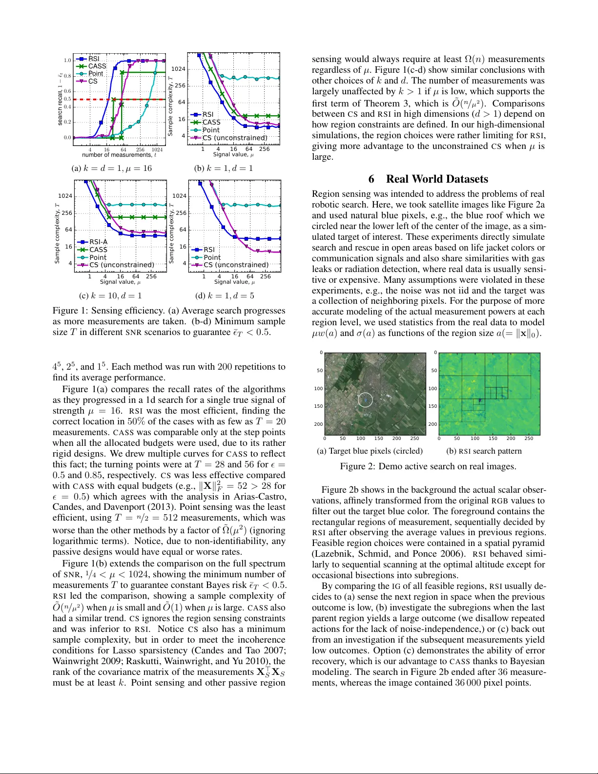
Activ e Sear ch f or Sparse Signals with Region Sensing Y ifei Ma Carnegie Mellon Uni v ersity Pittsbur gh P A 15213, US yifeim@cs.cmu.edu Roman Garnett W ashington University in St. Louis St. Louis, MO, USA garnett@wustl.edu Jeff Schneider Carnegie Mellon Uni v ersity Pittsbur gh P A 15213, US schneide@cs.cmu.edu Abstract Autonomous systems can be used to search for sparse signals in a large space; e.g., aerial robots can be deployed to localize threats, detect gas leaks, or respond to dist ress calls. Intuitiv ely , search algorithms may increase efficiency by collecting ag- gregate measurements summarizing lar ge contiguous regions. Howe ver , most existing search methods either ignore the possi- bility of such region observations (e.g., Bayesian optimization and multi-armed bandits) or make strong assumptions about the sensing mechanism that allow each measurement to ar- bitrarily encode all signals in the entire environment (e.g., compressiv e sensing). W e propose an algorithm that acti vely collects data to search for sparse signals using only noisy measurements of the average values on rectangular regions (including single points), based on the greedy maximization of information gain. W e analyze our algorithm in 1d and sho w that it requires ˜ O ( n / µ 2 + k 2 ) measurements to recover all of k signal locations with small Bayes error , where µ and n are the signal strength and the size of the search space, respecti vely . W e also sho w that active designs can be fundamentally more efficient than passiv e designs with region sensing, contrast- ing with the results of Arias-Castro, Candes, and Dav enport (2013). W e demonstrate the empirical performance of our algorithm on a search problem using satellite image data and in high dimensions. 1 Introduction Active sear ch describes the problem where an agent is giv en a target to search for in an unkno wn environment and acti vely makes data-collection decisions so as to locate the target as quickly as possible. Examples of this setting include using aerial robots to detect gas leaks, radiation sources, and human surviv ors of disasters. The statistical principles for ef ficient designs of measurements date back to Gergonne (1815), b ut the growing trend to apply automated search systems in a variety of en vironments and with a variety of constraints has drawn much research attention recently , due to the need to address the disparate aspects of new applications. One possibility in such acti ve search scenarios we aim to explore, inspired by the robotic aerial search setting but with statistical insights that we hope to generalize, is the opportunity to take aggreg ate measurements that summarize Copyright c  2017, Association for the Adv ancement of Artificial Intelligence (www .aaai.org). All rights reserved. large contiguous regions of space. For example, an aerial robot carrying a radiation sensor will sense a region of space whose area depends on its altitude. Ho w can such a robot dynamically trade off the ability to make noisier observ a- tions of larger regions of space against making higher -fidelity measurements of smaller regions? T o simplify the discussion, we will limit such r e gion sens- ing observations to re veal the average v alue of an underlying function on a rectangular region of space, corrupted by inde- pendent observ ation noise. Noisy binary search is a simple realization of active search using such an observation scheme. This mechanism turns out to be sufficiently informative in the cases that we analyze to offer insights into a variety of search problems. The ability to make aggregate re gion measurements in noisy en vironments has rarely been considered in previous work. Bayesian optimization, which has been used for local- ization of sparse signals (Carpin et al . 2015; Ma et al . 2015; Hernández-Lobato, Hoffman, and Ghahramani 2014; Jones, Schonlau, and W elch 1998), usually considers only point measurements of an objectiv e function. Notice that point ob- serv ations can be considered in our framew ork if the allowed region sensing actions are constrained to be arbitrarily small. On the other extreme, compressive sensing (Donoho 2006; Candès and W akin 2008; W ainwright 2009), considers scenar- ios where e very measurement can rev eal information about the entire en vironment through linear projection with arbi- trary coefficients. This is not al ways a realistic assumption, as for example for an aerial robot, which can only sense its im- mediate vicinity . Between the two extremes, Jedynak, Frazier, and Sznitman (2012); Rajan et al . (2015); Haupt et al . (2009); Carpentier and Munos (2012); Abbasi-Y adkori (2012); Y ue and Guestrin (2011) considered policies for search where ob- servations can be made on an y arbitrary subset of the search space, including discontiguous subsets, which is also often incompatible with the constraints in physical search systems. Another assumption we mak e, common for e xample in compressiv e sensing, is sparsity . W e assume that there are only a small number of strong signals in the environment; our goal is to recover these signals. Sparsity is necessary for the definition of activ e search problems; otherwise, for dense or weak signals, there is usually no better search approach than simply exhausti vely mapping the entire space. In addition to applicability in real search settings, spar- sity has unique mathematical properties when considered alongside region sensing. In unconstrained sensing, Arias- Castro, Candes, and Dav enport (2013) discovered a paradox that activ e compressi ve sensing (that is, the ability to adap- tiv ely select observations based on previously collected data) does not impro ve detection ef ficiency beyond logarithmic terms over random compressi ve sensing. This limitation is seen also when considering theoretical detection rates for activ e compressiv e sensing methods (Abbasi-Y adkori 2012; Carpentier and Munos 2012; Haupt et al . 2009). Howe ver , we sho w that activ e learning can in fact of fer significant improv e- ments in detection rates when observ ations are constrained to contiguous regions. W e propose an algorithm we call Re gion Sensing Index ( R S I ) that activ ely collects data to search for sparse signals using only noisy region sensing measurements. R S I is based on greedy maximization of information gain. Although infor- mation gain is a classic principle, we believe that its use in the recov ery of sparse signals is nov el and a good fit for robotic applications. W e show that R S I uses ˜ O ( n / µ 2 + k 2 ) measure- ments to recover all of k true signal locations with small Bayes error , where µ and n are the signal strength and the size of the search space, respectively (Theorem 3). The num- ber of measurements with R S I is comparable with the rates offered by unconstrained compressiv e sensing, ev en though our constraints seem strong (i.e., region sensing loses all spatial resolution inside the region of measurement). Further- more, we show that all passi ve designs under our contiguous region sensing constraint in 1 d search spaces are fundamen- tally worse, with ef ficiency no better than sequential scanning of e very point location, howe ver strong the signals are. These results provide e vidence to promote the use of and research into activ e methods. 1.1 Related W ork Arias-Castro, Candes, and Dav enport (2013) proved that the minimax sample complexity 1 for any (i.e., potentially adap- tiv e) algorithm to recover k sparse signal locations is at least Ω( n / µ 2 ) , analyzing the problem in terms of the mean-squared error in the recovery of the underlying signal values. The authors also showed that a passiv e random design, combined with a nontri vial inference algorithm, e.g., Lasso (W ainwright 2009) or the Dantzig selector (Candes and T ao 2007), can hav e similar recovery rates (up to O (log n ) terms). This result was presented as a paradox, suggesting that the folk statement that active methods have better sample complex- ity is not always true. Here we show that activ e search can make a substantial dif ference in reco very rates when the mea- surements are subject to the physically plausible constraint of region sensing, especially if the physical space has low dimensions. Malloy and No wak (2014) presented the first active search algorithm that achie ves the minimax sample comple xity for general k . The algorithm is called Compressi ve Adaptiv e Sense and Search ( C A S S ) and it can be adapted to region sensing in one-dimensional physical spaces. C A S S directly 1 Sample complexity is equiv alent to the number of measure- ments. extends bisection search, by allocating dif ferent sensing bud- gets to measurements at different bisection levels so as to minimize the cumulativ e error rates. Ho we ver , C A S S may fail if the repeated measurements of the same regions do not contain perfectly independent noise. It also has the lim- itation that it requires knowledge of the sensing budget a- priori , yet produces no signal localization results until the very last measurements at the lowest level. Our paper ad- dresses these practical issues with a redesigned active search algorithm using the Bayesian approach, which compares e v- idence instead of blindly trust the assumptions, and we use Shannon-information criteria, which implies bisection search in noiseless one-sparse cases. Braun, Pokutta, and Xie (2015) also used Shannon- information criteria for activ e search but did not analyze their sample complexity under noisy measurements. Jedynak, Frazier , and Sznitman (2012); Rajan et al . (2015) studied a similar search problem where the “regions” are relaxed to any unions of disjoint subsets. 2 Problem F ormulation Consider a discrete space that is the Cartesian product of one-dimensional grids, X = Q d i =1 [ n i ] ; [ n ] = { 1 , . . . , n } . Let n = Q n i be the total number of points in X (here the product symbol is the arithmetic rather than the Cartesian product). W e presume there is a latent real-valued nonne ga- tiv e vector β ∈ R n that represents the vector of true signals at all locations in X . W e further assume that β is sparse: it has v alue µ > 0 on k  n locations in X and has v alue 0 elsewhere. W e consider making observations related to β through rectangular region sensing measurements, defined by y t = x > t β + ε t , s . t . x tj = w t 1 j ∈ A t , ε t ∼ N (0 , σ 2 t ) . (1) Here x t ∈ R n is a sensing vector that has support on A t ⊆ X , a rectangular subset of X . W e assume that the sensing vector has equal weight w t across its support. The resulting measurement, y t , is equal to the mean value of β on A t corrupted by independent Gaussian noise with variance σ 2 t . Note that selecting A t suffices to specify the measurement location. In 1 d search environments, A t may be any interval of [ n ] , and the corresponding design takes the form x t = (0 , . . . , 0 , w t , . . . , w t , 0 , . . . , 0) > . In higher search dimen- sions, we consider only regions that are contained in a hierar- chical spacial pyramid (Lazebnik, Schmid, and Ponce 2006), i.e., a sequence of increasingly finer grid boxes with dyadic side lengths to cov er the space at multiple resolutions. Our goal is to choose a sequence of designs X = { x t } T t =1 so as to discov er the support of β with high confidence. Giv en a particular confidence, we will measure sample complex- ity by assuming k x t k 2 = 1 and σ t ≡ 1 for each measure- ment and count the total number of measurements required to achiev e that confidence, T . Letting k x t k 2 = 1 implies w t = 1 / √ k x t k 0 , which can be seen as a relaxed notion of the region average, because the signal strength of a region measurement, which is µw t , still decreases as the region size k x t k 0 increases. Algorithm 1 Region Sensing Inde x ( R S I ) Require: π 0 ( k , n, µ ) , T or  , and the unknown β ∗ Ensure: ˆ S t // (5) 1: for t = 1 , 2 , . . . do 2: pick x t = arg max x ∈X I ( β ; y | x , π t − 1 ) // (3)&(4) 3: observe y t = x > t β ∗ + ε t 4: update π t ( β ) ∝ π t − 1 ( β ) p ( y t | β , x t − 1 ) // (2) 5: find (¯  t , ˆ S t ) = arg min | ˆ S | = k 1 k E  | ˆ S ∆ S | | π t  // (5) 6: break if t ≥ T or ¯  t <  , if either is defined The measure of T is made to be comparable with another common choice of sample complexity , the Frobenius norm of the entire design k X k 2 F , when the rows of X are normalized (Arias-Castro, Candes, and Da venport 2013). Howe ver , the normalization is often overlooked in classical compressiv e sensing, which allows algorithms to cheat in region sens- ing by making an enormous number of measurements of small weight and changing the sensing locations frequently . Another measure of complexity is to measure both k X k 2 F and the number of location changes simultaneously (Malloy and No wak 2014). Howe ver , our discretized counting of measurements is conceptually simpler . Our analysis is Bayesian and we will analyze performance in expectation, with prior β ∼ π 0 ( β ) , a uniform distribution on the model class, S µ  n k  , which includes all k -sparse mod- els with µ signal strength among n locations (i.e., it has  n k  possible outcomes). The Bayes risk will be measured by the expected Delta loss, ¯  T = 1 k E | S ∆ ˆ S T | , where ˆ S T is the best estimator of the k signal locations after T measurements and ∆ is the symmetric dif ference operator on a pair of sets. 3 Proposed Methods W e note that region sensing loses all spatial resolution in- side the region of measurement. Here we borrow ideas from noisy binary search, which has a similar property , and use information gain (IG) to driv e the observ ation process. W e name our algorithm Re gion Sensing Index ( R S I , Algorithm 1). Like other acti ve learning algorithms, R S I is a combination of an infer ence subroutine that constantly updates the distri- bution of β using the collected data and a design subroutine that chooses the next region to sense based on the latest information from the inference subroutine. The inference subroutine. W e use e xact Bayesian inference with a uniform prior π 0 ( β ) on the model class S µ  n k  . Denote the outcome of the first t measurements as D t = { ( x τ , y τ ) : 1 ≤ τ ≤ t } . Even though D t contains a dependent sequence of data collections, where x τ depends on D τ − 1 , ∀ τ , Bayesian inference decomposes into a series of efficient updates: π ( β | D t ) ∝ π ( β ) p ( D t | β ) = π 0 ( β ) Q t τ =1  p ( x τ | D τ − 1 ) p ( y τ | β , x τ )  ∝ π 0 ( β ) Q t τ =1 p ( y τ | β , x τ ) , (2) where p ( x τ | D τ − 1 ) is the design without kno wledge of the true β and thus dropped. Define π t ( β ) = π ( β | D t ) ; the updates ha ve the form π t ( β ) ∝ π t − 1 ( β ) p ( y t | β , x t ) = π t − 1 ( β ) φ ( y t − x > t β ) , where φ is the standard normal pdf. The design subroutine. The next sensing vect or , x t +1 ∈ X , is chosen to maximize the IG: I ( β ; y | x , π t ) = H ( y | x , π t ) − E  H ( y | x , β ) | π t  , (3) which is the dif ference between the entropy of the mar ginal distribution, p ( y | x , π t ) = R φ ( y − x > β ) π t ( β ) d β , and the expected entropy of the conditional distribution, p ( y | β ; x ) = φ ( y − x > β ) . The latter , i.e., the conditional distri- bution for an y realization of β , has fixed entropy: log √ 2 π e . Meanwhile, the marginal entropy has no closed-form solu- tions; instead, we use numerical integration. The numerical integration is rather straightforward, be- cause the marginal density function is analytical. From now on, we will assume that ( x , A, a, w x ) correspond to the same design (its sensing vector , its locations, its region size, and its sensing weight per coordinate, respecti vely). Define two new v ariables, λ = µw x (= µ / √ a ) and γ = x > β / λ , and one new parameter p = ( p 0 , . . . , p k ) > in (4) . The goal is to change the variable of the integration for the marginal density function of y to: p ( y | x , π t ) = Z π t ( β ) φ ( y − x > β ) d β = X k c =0 p c φ ( y − cλ ) = p ( y | λ, p ) , where p c = Pr( γ = c ) = X β : x > β = cλ π t ( β ) . (4) Notice, γ only has a finite number of choices: γ = | A ∩ S | ∈ { 0 , . . . , k } , where S is the nonzero support of β , because both x and β are constant on their respective supports ( x j = w x , ∀ j ∈ A and β j = µ, ∀ j ∈ S ). W e then numerically ev aluate H ( y | x , π t ) = H ( y | λ, p ) with the obtained (4). The Bayes estimator of signal locations. W e pick the k - sparse set ˆ S T to minimize the posterior risk: min | ˆ S | = k 1 k E  | ˆ S ∆ S | | π T  = 1 k X ˆ ı ∈ ˆ S E  1 { β ˆ ı =0 } | π T  , (5) where β ˆ ı is the ˆ ı -th element of β . In other words, R S I picks the top k locations where the posterior marginal expectation is the largest. When k = 1 , this is equiv alent to picking ˆ β T = arg max π T ( β ) . Otherwise, (5) yields the smallest Bayes risk ¯  ( D T ) gi ven an y collected data D T . 3.1 Accelerations In practice, holding  n k  models in memory can be infeasi- ble if k is lar ge, we can instead recover the support of β element-wise by repeatedly applying R S I assuming k = 1 . After the posterior distribution π t ( β (1) ) con verges to a point- mass distribution at the most-likely one-sparse model with sufficient confidence, we report its location and mov e on by 2 In real world experiments, we additionally estimate ˆ µ ˆ  using a point measurement on the inferred signal location for better model- ing. T able 1: Conditions and conclusions for sample complexity . Design T ype Region Sensing Algorithm Prior for Bayes Risk Min T to Guarantee ¯  T = 1 k E | S ∆ ˆ S T | ≤  Sample Complexity ∗ passiv e yes (any) π 0 ( µ → ∞ ) T ≥ n 2 (1 − n − 1 n − k  ) (Theorem 1) Θ( n ) Point sensing T ≤ n (1 − n − 1 n − k  ) (Corollary A.2) activ e no (any) ˜ π 0 T ≥ 4 n µ 2 (1 −  ) 2 (Theorem 2) Ω( n µ 2 ) † yes C A S S [2014] max risk (incl. π 0 ) T ≤ 20 n µ 2 log( 8 k  ) + 2 k log 2 ( n k ) ˜ O ( n µ 2 + k ) ‡ R S I (ours) π 0 ¯ T  ≤ 50( n µ 2 + k 2 9 ) log 2 ( 2  ) log ( n  ) (Theorem 3) ˜ O ( n µ 2 + k 2 ) ‡ ∗ Assume  = O (1) and k  n . † Shown for unconstrained sensing; binary search requires Ω(log 2 ( n ) + k ) additional measurements. ‡ log( n ) terms are left out. ¯ T  is defined differently; see Section 4.2 for details. Algorithm 2 Region Sensing Inde x-Any- k ( R S I - A ) Require: n, µ ,  , and the unknown β ∗ Ensure: ˆ S 1: initialize ˆ S = ∅ , ˆ β = 0 2: for k = 1 , 2 , . . . , do 3: infer π 0 ( β ( k ) ) ∝ Q t τ =1 p ( y τ | β ( k ) + ˆ β , x τ ) , ∀ β ( k ) ∈ { µ 1 j : j 6∈ ˆ S } 4: call ˆ S ( k ) = R S I ( π 0 , , β ∗ − ˆ β ) 5: aggregate ˆ S = ∪ c ≤ k ˆ S ( c ) and ˆ β = P ˆ  ∈ ˆ S ˆ µ ˆ  1 ˆ  . 2 removing the reported point from the search and recomputing the posterior distributions using the uniform prior , π 0 ( β (2) ) , on the new class, S µ  n − 1 1  . W e call this alternativ e algorithm Re gion Sensing Index- Any- k ( R S I - A , Algorithm 2) and use it in our simulations so that the computational cost is no longer e xponential in k . Notice, our analysis is for the unmodified R S I ; the statistical disadv antage of R S I - A is no more than O ( k ) , multiplicati vely . When implementing R S I - A , we also a void unnecessary numerical integration (3) , if the region is guaranteed to hav e inferior IG, indicated by its p vector (4) , which is easier to compute. W e use the fact that I ( γ ; y | p , λ ) with fixed λ > 0 is concav e in the probability simplex ∆ k = { p ∈ [0 , 1] k +1 : p > 1 = 1 } . Under k = 1 approximation, the region whose marginal probability p 1 = P x > β > 0 π ( β ) is closest to 0 . 5 will prov ably have the largest IG among all regions of the same size. Thus, we find the region with the highest IG in two steps: (1) compare the p 1 value for all regions for e very region size and (2) ev aluate the IG of only these regions with the best p 1 values (closest to 0 . 5 ) in their region sizes. 4 Theoretical Analysis in 1D The analysis is cleanest when the search space is 1d, where the regions can be an y integer interv als that subset [1 , n ] . W ithout loss of generality (WLOG), assume n is a multiple of k and n ≥ 2 k . Our goal is to find the smallest number of measurements, T , to guarantee a small Bayes risk ¯  T = 1 k E | S ∆ ˆ S T | ≤  . T able 1 summarizes our analysis. The sample complexity is best appreciated assuming µ  1 , k  n , and  = O (1) . A typical choice is  = 1 / 2 , i.e., the number of measurements to guarantee that half of the signal support can be recov ered on av erage. 4.1 Baseline Results Here we provide lower bounds on sample complexity . W e show that under re gion-sensing constraints, all passi ve meth- ods require T ≥ Ω( n ) measurements and acti ve methods require T ≥ Ω( n / µ 2 + k ) . When µ  1 , acti ve methods ha ve significant potential for impro vement o ver passi ve methods using region sensing, which contradicts with the vie w in un- constrained compressiv e sensing by Arias-Castro, Candes, and Dav enport (2013); Soni and Haupt (2014). Theorem 1 (Limits of any passiv e methods using region sensing) . Assume β has prior π 0 (uniform random on S µ  n k  ). Any passive method with T noiseless r egion measur ements on 1d must incur Bayes risk ¯  T ≥ n − k n − 1 (1 − 2 T n ) . T o guar antee ¯  T ≤  , T ≥ n 2 (1 − n − 1 n − k  ) is r equired. The proof is due to model identifiability , neglecting obser- vation noise. More details can be found in the appendix. It applies to any µ ≥ 0 and particularly µ → ∞ . Theorem 2 (Limits of any methods, (Arias-Castro, Candes, and Da venport 2013)) . Assume β has a slightly dif ferent prior , ˜ π 0 , that includes each location in X in the support of β independently with pr obability k / n . Any method (including active and non-r e gion-sensing) must have ¯  T ≥ 1 − µ 2 p T / n . T o guarantee ¯  T ≤  , T ≥ 4 n µ 2 (1 −  ) 2 is r equired. The proof can be found under Theorem 3 of (Arias-Castro, Candes, and Dav enport 2013). Arias-Castro, Candes, and Dav enport (2013) ga ve a minimax risk with similar terms by modifying ˜ π 0 to a least favorable prior on all models that are at most k -sparse. Howe ver , we only study Bayes risk for technical con venience. When using Theorem 2 for reference, notice the dif fer- ence between ˜ π 0 and π 0 that the former additionally treats the sparsity to be a random v ariable ˜ k with expectation k . From concentration inequalities, | ˜ k − k | ≤ O ( √ k ) , with high probability . While ˜ k and k are not directly comparable, Theorem 2 is still a useful baseline. Under region-sensing constraints, the number of measurements must also be at least Ω( k ) to allow visits to most of the nonzero locations at least once, in a nontrivial dra w of S where the signals are separated. W ith respect to Theorem 1, the point sensing or an y non- repeating region sensing will achie ve the optimal sample complexity (up to constant factors, see Appendix A for more details). For Theorem 2, the C A S S method published by Malloy and Nowak (2014) for activ e sensing with re gion constraints 3 acheiv es a nearly optimal rate in theory . T able 1 contains a detailed summary of the sample complexities of sev eral algorithms, including our own. 4.2 Main Result For technical conv enience, we directly express our main result in terms of the expected number of measurement that are actually taken so as to realize ¯  ( D T ) ≤  for a gi ven threshold  in an experiment. T aking T = T  as a random variable, the expected number of actual measurements is different from the pre-determined sampling budget that an algorithm fully consumes to guarantee a desirable a veraged risk (see Section 4.1). Ho wev er, it is a comparable alternati ve in Bayesian analysis, used by e.g., Lai and Robbins (1985); Kaufmann, K orda, and Munos (2012). When the objecti ve is constant  = O (1) , our result implies a deterministic budget requirement of the same order of complexity , T ≤  − 1 2 E T  2 , where  2 =  2 , by direct application of Markov’ s inequality . Theorem 3 (Sample comple xity of R S I ) . In active sear ch for k sparse signals with str ength µ in 1d physical space of size n ≥ 2 k (WLOG, assume n is a multiple of k ), given any  > 0 as toler ance of posterior Bayes risk, R S I using r e gion sensing has bounded expected number of actual measur ements, ¯ T  = E [min {T : ¯  ( D T ) ≤  } ] ≤ 50  n µ 2 + k 2 9  log 2  2   log  n   = ˜ O  n µ 2 + k 2  , (6) wher e the expectation is taken over the prior distrib ution and sensing outcomes. 4.3 Proof Sketch The proof for Theorem 3 hinges on an observation that the information gain (IG) where R S I makes measurements is con- sistently large, before acti ve search terminates with minimal Bayes risk. For example, the IG of any measurement in bi- nary search with k = 1 and noiseless observations is al ways O (log(2)) . Howe ver , IG is harder to approximate when the observations are noisy . Therefore, we first show an intuiti ve lower bound for IG. Recall notations from (4). 3 The original result in Malloy and No wak (2014) is stronger; it considers the maximum probability of support recovery mistak es, P ( S 6 = ˆ S ) ≤ δ , for any S that are k -sparse and any signals with at least µ strength. Proposition 4. The IG scor e of a re gion sensing design has lower bounds with r espect to its design parameters ( λ, p ) , as I ( γ ; y | λ, p ) ≥ 2 q c ¯ q c  2Φ  λ 2  − 1  2 ≥ 1 12 min { q c , ¯ q c } min { λ 2 , 3 2 } , ∀ 1 ≤ c ≤ k , (7) wher e q c = Pr( γ ≥ c ) = P κ ≥ c p κ , ¯ q c = 1 − q c , and Φ( u ) is the standar d normal cdf. The proof uses Pinsker’ s inequality and is giv en in Sec- tion B in the appendix. Notice using the common choice of Jensen’ s inequality will gi ve bounds in the opposite direction. T o formalizes our observation that the IG is bounded: Lemma 5. WLOG, assume n is a multiple of k and n ≥ 2 k . At any step, if the curr ent Bayes risk ¯  ( D ) >  , we can always find a r e gion A of size at most n k , such that λ 2 ≥ µ 2 a = kµ 2 n and  2 ≤ E [ γ | D ] ≤ 1 −  2 (we call this Condition E ), which further yields I ( γ ; y | λ, p ) ≥ I ∗  =  25 k min n k 2 µ 2 n , 3 2 o . (8) The way to find the region A that satisfies Condition E is giv en in Lemma B.5 in the appendix. The reason that Condi- tion E is sufficient for (8) can be deriv ed from Proposition 4 for k = 1 and Lemma B.6 in the appendix for k > 1 . Eq (8) shows the minimum decrease in the model entrop y in expectation after each measurement, starting from the maximum entropy of a uniform prior distribution, k log( n ) . Howe ver , the posterior entropy can nev er be neg ativ e, which implies a bound on the expected number of times that (8) can be applied, i.e. the expected number of measurements to reach  Bayes risk is 25 log ( n )  ( n µ 2 + k 2 9 ) . Lemma D.5 in the appendix shows some additional impro vements to obtain the logarithmic dependency of  in Theorem 3. 5 Simulation Studies W e ev aluated R S I or its approximation R S I - A when k > 1 . Other baseline algorithms include: • C A S S (compressiv e adapti ve sense and search) (Mallo y and Nowak 2014): a branch-and-bound algorithm that tra- verses the region hierarchy from top to down using pre- allocated budgets per le vel. W e count each x i as k x i k 2 2 region sensing measurements (rounded up to the next inte ger). • Point sensing: a passiv e design that uses exhaustiv e point measurements on all locations. • C S (compressiv e sensing) (Donoho 2006): a non-region- sensing design that dra ws x t ∼ N ( 0 , I ) and rescales k x t k 2 2 to 1 . C S then solves a con vex optimization problem to infer the nonzero signals, by minimizing P t k y t − x > t β k 2 2 + λ k β k 1 s.t. β ≥ 0 , where λ is chosen to produce e xactly k nonzero coefficients using the Lasso re gularization path. W e picked n = 1024 and various k (sparsity) and d (the dimension of the physical space) annotated belo w the plots. In the d = 5 case, we chose the region space to be the Cartesian product of [4] 5 and allowed re gions from a spatial pyramid (Lazebnik, Schmid, and Ponce 2006) of granularity 4 16 64 256 1024 n umber of measurements , t 0 . 0 0 . 2 0 . 4 0 . 5 0 . 6 0 . 8 1 . 0 search recall, 1 − ¯  t RSI CASS P oint CS (a) k = d = 1 , µ = 16 1 4 16 64 256 S i g n a l v a l u e , ¹ 4 16 64 256 1024 S a m p l e c o m p l e x i t y , T RSI CASS Point CS (unconstrained) (b) k = 1 , d = 1 1 4 16 64 256 S i g n a l v a l u e , ¹ 4 16 64 256 1024 S a m p l e c o m p l e x i t y , T RSI-A CASS Point CS (unconstrained) (c) k = 10 , d = 1 1 4 16 64 256 S i g n a l v a l u e , ¹ 4 16 64 256 1024 S a m p l e c o m p l e x i t y , T RSI Point CS (unconstrained) (d) k = 1 , d = 5 Figure 1: Sensing ef fi cienc y . (a) A v erage search progresses as more measurements are tak en. (b-d) Minimum sample size T in dif ferent S N R scenarios to guarantee ¯  T < 0 . 5 . 4 5 , 2 5 , and 1 5 . Each method w as run with 200 repetitions to find its a v erage performance. Figure 1(a) compares the recall rates of the algorithms as the y progressed in a 1d search for a single true signal of strength µ = 16 . R S I w as the most ef fi cient, finding the correct location in 50% of the cases with as fe w as T = 20 measurements. C A S S w as comparable only at the step points when all the allocated b udgets were used, due to its rather rigid designs. W e dre w multiple curv es for C A S S to reflect this f act; the turning points were at T = 28 and 56 for  = 0 . 5 and 0 . 85 , respecti v ely . C S w as less ef fect i v e compared with C A S S with equal b udgets (e.g., k X k 2 F = 52 > 28 for  = 0 . 5 ) which agrees with the analysis in Arias-Castro, Candes, and Da v enport (2013). Point sensing w as the least ef ficient, using T = n / 2 = 512 measurements, which w as w orse than the other methods by a f actor of ˜ Ω( µ 2 ) (ignoring log arithmic terms). Notice, due to non-identifiability , an y passi v e designs w ould ha v e equal or w orse rates. Figure 1(b) e xtends the comparison on the full spectrum of S N R , 1 / 4 < µ < 1024 , sho wing the minimum number of measurements T to guarantee constant Bayes risk ¯  T < 0 . 5 . R S I led the comparison, sho wing a sample comple xity of ˜ O ( n / µ 2 ) when µ is small and ˜ O (1) when µ is lar ge. C A S S also had a similar trend. C S ignores the re gion sensing constraints and w as inferior to R S I . Notice C S also has a minimum sample comple xity , b ut in order to meet the incoherence conditions for Lasso sparsistenc y (Candes and T ao 2007; W ainwright 2009; Raskutti, W ainwright, and Y u 2010), the rank of the co v ariance matrix of the meas urements X > S X S must be at least k . Point sensing and other passi v e re gion sensing w ould al w ays requir e at least Ω( n ) measurements re g ardless of µ . Figure 1(c-d) sho w similar conclusions with other choices of k and d . The number of measurements w as lar gely unaf fec ted by k > 1 if µ is lo w , which supports the first term of Theorem 3, whi ch is ˜ O ( n / µ 2 ) . Comparisons between C S and R S I in high dimensions ( d > 1 ) depend on ho w re gion constraints are defined. In our high-dimens ional simulations, the re gion choices were rather limiting for R S I , gi ving more adv antage to the unconstrained C S when µ is lar ge. 6 Real W orld Datasets Re gion sensing w as intended to address the problems of real robotic search. Here, we took satellite images lik e Figure 2a and used natural blue pix els, e.g., the blue roof which we circled near the lo wer left of the center of the image, as a s im- ulated tar get of interest. These e xperiments directly simulate search and rescue in open areas based on life jack et colors or communication signals and also share similarities with g as leaks or radiation detection, where real data is usually sensi- ti v e or e xpensi v e. Man y assumptions were violated in these e xperiments, e.g., the noise w as not iid and the tar get w as a collection of neighboring pix els. F or the purpose of more accurate model ing of the actual measurement po wers at each re gion le v el, we used statistics from the real data to model µw ( a ) and σ ( a ) as functions of the re gion size a (= k x k 0 ) . 0 50 100 150 200 250 0 50 100 150 200 (a) T ar get blue pix els (circled) 0 50 100 150 200 250 0 50 100 150 200 (b) R S I search pattern Figure 2: Demo acti v e search on real images. Figure 2b s ho ws in the background the actual scalar obser - v ations, af finely transformed from the original R G B v alues to filter out the tar get blue color . The fore ground contains the rectangular re gions of measurement, sequentially decided by R S I after observing the a v erage v alues in pre vious re gions. Feasible re gion choices were contained in a spatial p yramid (Lazebnik, Schmid, and Ponce 2006). R S I beha v ed simi- larly to sequential scanning at the optimal altitude e xcept for occasional bisections into subre gions. By comparing the I G of all feasible re gions, R S I usually de- cides to (a) sense t he ne xt re gi on in space when the pre vious outcome is lo w , (b) in v esti g ate the subre gions when the last parent re gion yields a lar ge outcome (we disallo w repeated actions for the lack of noise-independence,) or (c) back out from an in v est ig ation if the subsequent measurem ents yield lo w outcomes. Option (c) demonstrat es the ability of error reco v ery , which is our adv antage to C A S S thanks to Bayesian modeling. The search in Figure 2b ended after 36 measure- ments, whereas the image contained 36 000 pix el points. Figure 3 compares the performances on 221 image patches of 512 × 512 pix els, cropped from National Agriculture Im- agery Program (N AIP). 4 The other algorithms for comparison include random (point), C S , and C A S S * . Here, C A S S * is a modified C A S S method where each measurement can only be tak en once, because repeated measurements yield the sam e outcome. T o fully represent C A S S * , in addition to choosing k by the true sparsity , we added fix ed choices of k = 64 and 512 , yielding three dif ferent curv es. 0.1% 1.0% 10.0% percent feasible observations 0.0 0.2 0.4 0.6 0.8 1.0 signal recall rate RSI-A CASS* Point CS Figure 3: Performances on 221 N A I P image crops. R S I achie v ed the best per - formance, finding on a v er - age 60% blue pix els with as fe w as 1700 measure- ments ( 0 . 5% of the total number of feasible observ a- tions). C A S S * performance highly depended on the pa- rameter choices and pro- duced results only near the end of the e xperiment. C S did poorl y , probably due to the f act the signals were not iid (a blue object can contain multiple pix els). 7 Discussions Re gion sensing is a ne w setting moti v ated by robotic search operations where we also found statistical insights to contrast with the unconstrained sensing in Arias-Castro, Candes, and Da v enport (2013). R S I performs near -optimally in 1d search domains and fundamentally f aster than passi v e sensing. In higher dimensions, the analysis may be harder , especially for passi v e baselines. The number of subre gions generated by intersecting the measurement re gions may be harder to count, unless measurement re gions are restricted to grid re gions in a spatial p yramid (such that an y pair of re gions is either nested or disjoint). W e also w ant to establish frequentist analysis in t he future. Finally , it is interesting to generalize the measurement model be yond taking the a v erage v alue of a single re gion at a time. Ackno wledgments This w ork is partially supported by the D ARP A grant F A87501220324, National Science F oundation under A w ard Number IIA-1355406, and ARP A-E TERRA-REF a w ard DE- AR0000594. W e also appreciate suggestions and discussions from Aarti Singh, Y ing Y ang, and Y ining W ang. Refer ences Abbasi-Y adk ori, Y . 2012. Online-to-confidence-set con v ersions and application to sparse stochastic bandits. Arias-Castro, E.; Candes, E. J.; and Da v enport, M. 2013. On the fundamental limits of adapti v e sensing. Information Theory , IEEE T r ansactions on . Braun, G.; Pokutta, S.; and Xie, Y . 2015. Info-greedy sequential adapti v e compressed sensing. IEEE J ournal of Selected T opics in Signal Pr ocessing 9(4):601–611. 4 https://lta.cr.usgs.gov/node/300 Candes, E., and T ao, T . 2007. The dantzig selector: statistical estimation when p is much lar ger than n. The Annals of Statistics . Candès, E. J., and W akin, M. B. 2008. An introduction to compres- si v e sampling. Signal Pr ocessing Ma gazine , IEEE 25(2):21–30. Carpentier , A., and Munos, R. 2012. Bandit theory meets com- pressed sensing for high dimensional stochastic linear bandit. In AIST A TS , v olume 22, 190–198. Carpin, M.; Rosati, S.; Khan, M. E.; and Rimoldi, B. 2015. Ua vs using bayesian optimization to locate wifi de vices. arXiv pr eprint . Donoho, D. L. 2006. Compressed sensing. Information Theory , IEEE T r ansactions on 52(4):1289–1306. Ger gonne, J. D. 1815. Application de la méthode des moindre quarrés a l’interpolation des suites. Annales des Math Pur es et Appl . Haupt, J. D.; Baraniuk, R. G.; Castro, R. M.; and No w ak, R. D. 2009. Compressi v e distilled sensing: Sparse reco v ery usi ng adapti vity in compressi v e measurements. In Signals, Systems and Computer s . IEEE. Hernández-Lobato, J. M.; Hof f man, M. W .; and Ghahramani, Z. 2014. Predicti v e entrop y search for ef ficient global optimization of black-box functions. In Advances in Neur al Information Pr ocessing Systems . Jedynak, B.; Frazier , P . I.; and Sznitman, R. 2012. T wenty questions with noise: Bayes opti mal policies for entrop y loss. J ournal of Applied Pr obability 49(1):114–136. Jones, D. R.; Schonlau, M.; and W elch, W . J. 1998. Ef fi cient global optimization of e xpensi v e black-box functions. J ournal of Global optimization 13(4):455–492. Kaufmann, E.; K orda, N.; and Munos, R. 2012. Thompson sam- pling: An asymptotically optimal finite-time analysis. In Algorith- mic Learning Theory , 199–213. Springer . Lai, T . L., and Robbins, H. 1985. Asymptotically ef ficient adapti v e allocation rules. Advances in applied mathematics 6(1):4–22. Lazebnik, S.; Schmid, C.; and Ponce, J. 2006. Be yond bags of features: Spatial p yramid matching for recognizing natural scene cate gories. In Computer V ision and P attern Reco gnition . IEEE. Ma, Y .; Sutherland, D.; Garnett, R.; and Schneider , J. 2015. Ac- ti v e pointillistic pattern search. In Pr oceedings of the Eighteenth International Confer ence on Artificial Intellig ence and Statistics . Mallo y , M. L., and No w ak, R. D. 2014. Near -optimal adapti v e compressed sensing. Information Theory , IEEE T r ansactions on . Rajan, P .; Han, W .; S znitman, R.; Frazier , P .; and Jedynak, B. 2015. Bayesian multiple tar get localization. In Pr oceedings of the 32nd International Confer ence on Mac hine Learning (ICML) . Raskutti, G.; W ainwright, M. J.; and Y u, B. 2010. Restricted eigen v alue properties for correlated g aussian designs. The J ournal of Mac hine Learning Resear c h . Soni, A., and Haupt, J. 2014. On the fundamental limits of reco v er - ing tree spars e v ectors from noisy linear measurements. Information Theory , IEEE T r ansactions on . W ainwright, M. J. 2009. Sharp t hresholds for high-dimensional and noisy sparsity reco v ery using-constrained quadratic programming (lasso). Information Theory , IEEE T r ansactions on . Y ue, Y ., and Guestrin, C. 2011. Linear submodular bandits and their application to di v ersified retrie v al. In Advances in Neur al Information Pr ocessing Systems , 2483–2491. Activ e Sear ch f or Sparse Signals with Region Sensing (Appendix) Y ifei Ma Carnegie Mellon Uni versity Pittsbur gh P A 15213, US yifeim@cs.cmu.edu Roman Garnett W ashington University in St. Louis St. Louis, MO, USA garnett@wustl.edu Jeff Schneider Carnegie Mellon Uni versity Pittsbur gh P A 15213, US schneide@cs.cmu.edu Abstract This supplementary material includes both theoretical details ( Section A–B ) and additional empirical results ( Section C ). For the theoretical part, our main paper has two separate results: a hardness result sho wing passiv e methods under re gion sensing constraints in 1d search spaces cannot be ef ficient (Theorem 1 and the first row in T able 1 in the main paper) and a positi ve result showing that our Re gion Sensing Index ( R SI ) is sample-efficient (Theorem 3), comparable with the optimal ef ficiency obtained in (Arias-Castro, Candes, and Dav enport 2013). The empirical part contains the choice of parameters and a demo of search results. For conv enience, in the appendix, we sometimes use K to represent the total number of sparse signals in the system, whereas in the main document we always used k . A Theoretical Pr operties for P assive Sensing Theorem A.1 ( Theorem 1 in the main document; limits of any passive methods using region sensing) . Assume β has prior π 0 (uniform random on S µ  n k  ). Any passive method with T noiseless r egion measur ements on 1D must incur Bayes risk ¯  T ≥ n − k n − 1 (1 − 2 T n ) ; to guarantee ¯  T ≤  , it r equires T ≥ n 2 (1 − n − 1 n − k  ) . Pr oof. W e count the number of non-identifiability models with T noiseless observations, particularly when T < n 2 . An aggre gate measurement on region [ a i , b i ) ⊂ [1 , n + 1) cannot identify the sparse support inside [ a i , b i ) (or its complement), unless it intersects with another aggregate measurement. Should two measurement regions intersect, the model is still non- identifiable inside the intersection, set differences, and the complement of the union of both. T o find out the set of all disjoint subsets where the model is non-identifiable giv en any passiv e design with m region measurements, { [ a i , b i ) ⊂ [1 , n + 1) : i = 1 , . . . , m } , we simply sort the unique end points as c 1 < · · · < c p ∈ { a i , . . . , a m } ∪ { b 1 , . . . , b m } , where p ≤ 2 m , and use the following set of p elementary subsets:  [ c j , c j +1 ) | {z } C j : j = 1 , . . . , p − 1  ∪  [ c p , n + 1) ∪ [1 , c 1 ) | {z } C p  , (A.1) where the last subset is created to ensure that the number of sparse supports in the full set equals k . Notice, (A.1) is also the largest set of disjoint subsets that can be created using intersections, unions, and complements on the regions of measurements. W e will continue our discussion assuming that the measurements are made on the subsets contained in (A.1). When the observations are noiseless, (A.1) is a superior design than the original design, whose outcomes can be inferred as x > [ a i ,b i ) β = p − 1 X j =1 c j +1 − c j b i − a i x > [ c j ,c j +1 ) β . (A.2) At this point, it is easy to see that the minimum sample size to guarantee that the signals can be fully identifiable in the worst case is T ≥ n 2 ; the necessary (and sufficient) condition is to ha ve | C j | = 1 , ∀ j = 1 , . . . , p , which requires 2 T ≥ p ≥ n . For  > 0 , we compute the expected Delta-risk giv en any fixed design which yields p elementary subsets as shown in (A.1). Let n j = | C j | , j = 1 , . . . , p . If the model β distributes k j supports in subset C j , respectively , then on any re gion where Copyright c  2017, Association for the Advancement of Artificial Intelligence (www .aaai.or g). All rights reserved. n j > k j > 0 , the inference algorithm can only make a random guess, e.g., for the first k j elements. Let β C j be the signal vector on subset C j , the conditional expected error on this subset is: E  | β C j ∆ ˆ β C j | | k j  = k j X e j =1  n j − k j e j  k j k j − e j   n j k j  e j = k j X e j =1  n j − k j − 1 e j − 1  k j k j − e j   n j k j  ( n j − k j ) =  n j − 1 k j − 1   n j k j  ( n j − k j ) = k j ( n j − k j ) n j . (A.3) The total risk conditioned on all of k j : j = 1 , . . . , p is: E  | β ∆ ˆ β | | k 1 , . . . , k p  = p X j =1 E  | β C j ∆ ˆ β C j | | k j  = p X j =1 k j ( n j − k j ) n j . (A.4) Using the law of total expectation assuming β to be uniformly distributed, we can compute the expected error of the given passiv e design as E | β ∆ ˆ β | = X k 1 + ··· + k p = K Q p j =1  n j k j   n K  ! p X j =1 k j ( n j − k j ) n j ! = p X j =1 X k 1 + ··· + k p = K Q p j 0 =1  n j 0 k j 0   n K  k j ( n j − k j ) n j = p X j =1 X k 1 + ··· + k p = K ( n j − 1)  n j − 2 k j − 1  Q j 0 6 = j  n j 0 k j 0   n K  = p X j =1 ( n j − 1)  n − 2 K − 1   n K  = ( n − p )  n − 2 K − 1   n K  = K ( n − K ) n ( n − 1) ( n − p ) ≤ K ( n − K )( n − 2 T ) n ( n − 1) (A.5) T o guarantee E | β ∆ ˆ β | ≤ K  , by solving (A.5) ≤ K  , a passiv e design requires a minimal sample size of T ≥ p 2 ≥ n 2  1 − n − 1 n − K   . (A.6) Corollary A.2. Using noiseless r egion-sensing observations, a passive design in 1D with T ≤ n 2 r egion measur ements achie ves the optimal averag e-case Delta-risk, if and only if it can separ ate the sear ch space into 2 m disjoint subsets using intersections, unions, and complements of the measur ement re gions. The following example is adapted fr om Gray code: t x > 1 0 0 0 0 1 1 1 1 2 0 0 1 1 1 1 0 0 3 0 1 1 0 0 0 0 0 4 0 0 0 0 0 1 1 0 · · · · · · (the pattern cycles) (A.7) Pr oof. T o minimize (A.5), it is suf ficient to find passive designs where p = 2 T , giv en that the region aggregate measurements are noiseless. The expected risk of (A.5) turns out to be independent of the sizes of each elementary subset C j (which one can verify with a minimal example where n = 4 , K = 2 , and p = 2 ), which suggests that all designs that yield p = 2 T have the same av erage-case Delta-risk with noiseless region aggregate measurements. Notice that the Gray-code design may not be optimal when the measurements are noisy . For this reason, we also included point sensing in T able 1 in our main paper, which yields the same order of sample complexity and performs better when the measurement noise is large. B Theoretical Pr operties for Acti ve Sensing The main goal of this section is to show that our main algorithm, Region Sensing Inde x ( R S I ), has the sample complexity guarantees show as Theorem 3 in the main paper . The main paper includes a proof sketch with three major steps. W e show their details in 3 respectiv e subsections. B.1 Basic Properties of Inf ormation Gain (IG) Recall that the observ ation model is y t = x > t β +  t , where β ∈ S µ  n k  , β ∼ π t , and  t ∼ N (0 , σ 2 t ) . Omitting the time index t in this subsection, the information gain (IG) to be maximized in e very step is defined as I ( β ; y | x , π ) = H ( y | x , π ) − E [ H ( y | x , β ) | π ] ⇔ I ( γ ; y | λ, p ) = H ( y | λ, p ) − H (  ) , (B.1) where f ( y | λ, p ) = K X c =0 p c φ ( y − cλ ) λ = µw x , γ = x > β λ , p c = Pr( γ = c ) = X β : x > β = cλ π t ( β ) . (B.2) There are two basic properties: Lemma B.1 that is both directly applied in Section 3.1 Accelerations and indirectly used in the later proof sketch; and Proposition B.2 that appears as Proposition 4 in the main paper . Basic Property 1 Lemma B.1 (Concavity and monotonicity) . I ( γ ; y | λ, p ) is concave in p ∈ R K +1 + , which includes the conve x simplex of ∆ K = { p ∈ [0 , 1] K +1 : p > 1 = 1 } , if 0 < λ < ∞ r emains constant. On the other hand, I ( γ ; y | λ, p ) with fixed p ∈ ∆ K is monotone-incr easing as λ increases. Pr oof. Conca vity and monotonicity can be verified using deri vati ves. Notice the second term in (B.1) is constant. Here are the equations for the first term as well as its first and second order deriv ativ es, omitting the dependency on p and λ for simplicity: H ( y ; λ, p ) = − Z f ( y ) log f ( y )d y , (B.3) ∂ H ( y ; λ, p ) = − Z  1 + log f ( y )  ∂ f ( y ) d y, (B.4) ∂ 2 H ( y ; λ, p ) = − Z  ∂ f ( y ) ∂ f ( y ) > f ( y ) +  1 + log f ( y )  ∂ 2 f ( y )  d y (B.5) Part 1. T o show concavity in p ( ≥ 0) , let φ λ ( y ) = ( φ ( y ) , φ ( y − λ ) , . . . , φ ( y − K λ )) > and write out the gradient and the Hessian of H ( y ; λ, p ) with respect of p as: ∂ H ( y ; λ, p ) ∂ p > = − Z ∞ −∞  1 + log f ( y )  φ λ ( y ) d y (B.6) ∂ 2 H ( y ; λ, p ) ∂ p ∂ p > = − Z ∞ −∞ 1 f ( y ) φ λ ( y ) φ λ ( y ) > d y (B.7) Notice φ λ ( y ) φ λ ( y ) > is a PSD Gram matrix, which is preserved under integration. Further , the integral returns a PD matrix if the distribution is not de generate ( λ > 0 and p k > 0 for at least two distinct k s) Part 2.1 For monotonicity in λ ( > 0) , in the case when K = 1 , the deri vati ve with respect to λ is ∂ H ( y ) ∂ λ = − Z  1 + log f ( y )  · p 1 φ ( y − λ ) · ( y − λ ) d y = − p 1 Z log f ( y ) · φ ( y − λ ) · ( y − λ ) d y = − p 1 Z log f ( y + λ ) · φ ( y ) · ( y ) d y, (B.8) where the first line removes constant integrals and the second shifts the variable. In order to show that (B.8) is nonnegativ e, pair up y and − y for y > 0 and notice that, by assuming λ > 0 , φ ( y + λ ) ≤ φ ( − y + λ ) ⇒ f ( y + λ ) ≤ f ( − y + λ ) . The bigger λ , the larger deri vati ve it has. Part 2.2 In general when K ≥ 1 , we can write out the deriv ativ e as ∂ H ( y ; λ, p ) ∂ λ = − Z ∞ −∞  1 + log f ( y )  K X k =0 p k φ ( y − k λ )( y − k λ ) k d y = − K X k =1 Z ∞ −∞ (1 + log f ( y )) K X t = k p t φ ( y − tλ )( y − tλ ) d y (B.9) Define h k ( y ) = P K t = k p t φ ( y − tλ ) ; we have 0 = − h k ( y ) log h k ( y )    ∞ −∞ = Z ∞ −∞ (1 + log h k ( y )) K X t = k p t φ ( y − tλ )( y − tλ ) d y (B.10) Consider each term of k in (B.9) and add the corresponding terms from (B.10); using ` k = P k − 1 s =0 p s φ ( y − sλ ) , we get ∂ H ( y ; λ, p ) ∂ λ = − K X k =1 Z ∞ −∞ log 1 + ` k ( y ) h k ( y ) ! K X t = k φ ( y − tλ )( y − tλ ) d y . (B.11) The only remaining task is to sho w that r k ( y ) = ` k ( y ) h k ( y ) is monotone decreasing with respect to y , which is sufficient to guarantee that (B.11) ≥ 0 , due to the odd symmetry of the remaining integrand parts around y = tλ . T ake the deriv ativ e of r k ( y ) with respect to y : r 0 k ( y ) = ` 0 k ( y ) h k ( y ) − ` k ( y ) h 0 k ( y ) h 2 k ( y ) = P s 0 and p k 6 = 0 for at least two k ∈ { 0 , . . . , K } . Basic Property 2 Proposition B.2 ( Pr oposition 4 in the main document; a lo wer bound for the IG of a design) . The IG scor e of a r e gion sensing design has lower bounds with r espect to its design parameters ( λ, p ) , as I ( γ ; y | λ, p ) ≥ 2 q c ¯ q c (2Φ( λ 2 ) − 1) 2 ≥ 1 12 min { q c , ¯ q c } min { λ 2 , 3 2 } , ∀ 1 ≤ c ≤ K , (B.13) wher e q c = P ( γ ≥ c ) = P κ ≥ c p κ , ¯ q c = 1 − q c , and Φ( u ) is the standar d normal cdf. Pr oof of Pr oposition B.2. T o show (B.13) , first inequality: Pick any 1 ≤ c ≤ K ; let v = 1 γ ≥ c and ˆ v = 1 y > ( c − 1 / 2 ) λ be two binary truncations of the original variables, γ and y , respectiv ely . These truncations lose information: I ( γ ; y | p , λ ) ≥ I ( v ; ˆ v | p , λ ) = E v K  ( ˆ v | v ) k ˆ v  ≥ 2 X v 0 ∈{ 0 , 1 } P ( v = v 0 ) sup ˆ v 0   P ( ˆ v = ˆ v 0 | v = v 0 ) − P ( ˆ v = ˆ v 0 )   | {z } , ˆ δ ( v 0 , ˆ v 0 ) 2 , (B.14) where K ( · k · ) is the Kullback–Leibler di vergence and the second line comes from Pinsk er’ s inequality . Consider any realization of v = v 0 and choose ˆ v 0 = v 0 ; using the rule of total probability and direct calculation, ˆ δ ( v 0 , v 0 ) =    P ( ˆ v = v 0 | v = v 0 ) − P ( v = v 0 ) P ( ˆ v = v 0 | v = v 0 ) − P ( v 6 = v 0 ) P ( ˆ v = v 0 | v 6 = v 0 )    = P ( v 6 = v 0 )    P ( ˆ v = v 0 | v = v 0 ) − P ( ˆ v = v 0 | v 6 = v 0 )    ≥ P ( v 6 = v 0 ) h Φ  λ 2  −  1 − Φ  λ 2 i = P ( v 6 = v 0 )  2Φ  λ 2  − 1  , (B.15) where Φ( λ 2 ) is a l o wer bound on the probabil ity of correct estimation, based on the w orst-case dra w of γ such that y cannot be more than λ 2 a w ay from γ in the direction that leads to estimation errors. T aking (B.15) to (B.14) yields t he first part of the result. T o sho w (B.13) , second inequality: So f ar we ha v e sho wn an analytical lo wer bound for I ( γ ; y | λ, p ) . T o mak e the result e v en more interpretable, we can further numerically e v aluate the Gaussian tai l distrib ution, to find t w o constants, C 1 and C 2 , such that Φ( x ) − 1 2 = Z x 0 φ ( u ) d u = Z x 0 1 √ 2 π e − u 2 2 d u ≥ C 1 min { x, C 2 } . (B.16) Since Φ( x ) is monotone-increasing, we can fix C 2 to find the w orst dif ference quotient, Φ( x ) / x , ∀ x ∈ (0 , C 2 ] . In f act, we can directly assign C 1 ≤ Φ( C 2 ) / C 2 , because φ ( u ) is monotone-decreasing as u increases. W e choose C 2 = 3 2 and C 1 = 1 √ 12 , which yields  2Φ  λ 2  − 1  2 ≥ 1 12 min  λ 2 , 3 2  . (B.17) Pr oposition B.3 (An upper bound for the IG of a design) . When K = 1 and WLOG p 1 ≤ 1 2 , the upper bound of IG derived fr om J ensen’ s inequality and max-entr opy principle is I ( γ ; y | λ, p ) ≤ 1 2 p 1 λ 2 , whic h is on the same or der of (B.13) when λ < O (1) . In the λ  1 case , the IG is natur ally upper -bounded by a Bernoulli e xperiment with noiseless observati on, H ( B ( p 1 )) = − p 1 log ( p 1 ) − (1 − p 1 ) log (1 − p 1 ) = ˜ O ( p 1 ) . Ther efor e , Pr oposition B.2 is a good appr oximation to the true IG in all scenarios. (See F igur e 1 for an empirical visualization.) The g ener al upper bound is not tight for g ener al k > 1 . Pr oof. The upper bound can be sho wn by Jensen’ s inequality and max-entrop y principle. It is also tight when k = 1 . Omitting p and λ , I ( γ ; y ) = I ( γ ; γ +  ) = H ( γ +  ) + H ( γ +  | γ ) = H ( γ +  ) − H (  ) . (B.18) W e only need to find the lar gest entrop y for H ( γ +  ) gi v en p and λ . By Jensen’ s inequality , under the same mean and v ariance, a normal distrib ution has the lar gest entrop y , where we ha v e: E ( γ +  ) = E ( γ ) + E (  ) = p 1 λ, σ 2 mar = V ar( γ +  ) = V ar( γ ) + V ar(  ) + 2Co v ( γ ,  ) = p 1 λ 2 + 1 . (B.19) W e can then use a normal distrib ution with the abo v e mean and v ariance as a upper bound to: I ( γ ; y ) = H ( γ +  ) − H (  ) ≤ 1 2 log (2 π eσ 2 mar ) − 1 2 log (2 π e ) = 1 2 log (1 + p 1 λ 2 ) ≤ 1 2 p 1 λ 2 (B.20) 1 0 - 2 1 0 - 1 1 0 0 1 0 1 1 0 2 λ 1 0 - 8 1 0 - 7 1 0 - 6 1 0 - 5 1 0 - 4 1 0 - 3 1 0 - 2 1 0 - 1 p 1 1.0e-09 1.0e-07 1.0e-05 1.0e-03 1.0e-01 information gain Figure 1: Le v el sets of IG I ( γ ; y | λ, p 1 ) for dif ferent v alues of p 1 and λ , when k = 1 . The thin lines belo w each true v alue indicate IG upper bounds (Proposition B.3) and the dashed lines are the phase-changing lo wer bound from Proposition B.2. The phase-changing bound is more useful because it produces insights about optimal re gion selection, usually at the point of phase-change, whereas the upper bound is non-informati v ely linear in the log-log plot. B.2 Minimum Inf ormation Gain of the Chosen Region in Each Iteration This subsection aims to formalize the main observ ation in our main paper , which is that the information gain of all of the chosen measurements from R S I remain consistently large, before activ e search terminates with minimal Bayes risk. This observation implies a constant speed at which the model uncertainty can be reduced in expectation, leading to the upper bounds on sample complexity in Section B.3. Recall that the Bayes risk is defined by ¯  t = min | ˆ S | = k 1 k E [ | ˆ S ∆ S | | π t ] , where ∆ is the symmetric set dif ference operator . If we include the Bayes inference rule π t ( β ) ∝ π 0 ( β ) Q t τ =1 p ( y | x τ , β ) , we can see that ¯  t is essentially a function of the collected data D t = { ( x τ , y τ ) : 1 ≤ τ ≤ t } . The following lemma paraphrases Lemma 5 in the main document, with the time index t omitted. Lemma B.4 (Minimum IG of the chosen regions) . WLOG, assume n is a multiple of 2 k . At any step, given the data collection outcomes D and the curr ent Bayes risk ¯  ( D ) , we can always find a r e gion A of size at most n k , such that λ 2 ≥ µ 2 a = kµ 2 n and ¯  ( D ) 2 ≤ E [ γ A | D ] ≤ 1 − ¯  ( D ) 2 (we call it Condition E ), which further yields I ( γ ; y | λ, p ) ≥ I ∗ ¯  = ¯  ( D ) 25 k min { k λ 2 , 3 2 } ≥ ¯  ( D ) 25 k min { k 2 µ 2 n , 3 2 } . (B.21) Condition E Lemma B.4 states the result in two steps: (a) the fact that the posterior model after collecting data D still has large Bayes risk implies the existence of a very informative region that satisfies Condition E and (b) sensing on this region indeed yields nontrivial information, measured in terms of IG (B.21). W e will split the proof into these two steps, accordingly . Lemma B.5 (A region that satisfies Condition E ) . In 1d sear ch with unit ` 2 -norm measurements, WLOG, assume n is a multiple of 2 k . At any step, given the collected data D and the curr ent Bayes risk ¯  ( D ) : 1. Ther e always is a re gion B of size no larg er than n k , such that λ 2 B ≥ µ 2 | B | = kµ 2 n and E [ γ B | D ] ≥ ¯  ( D ) 2 2. Ther e always is a subre gion A ⊂ B that satisfies Condition E : λ 2 A ≥ k µ 2 n and ¯  ( D ) 2 ≤ E [ γ A | D ] ≤ 1 − ¯  ( D ) 2 (B.22) Pr oof. Part 1. Suppose the current minimizer of the posterior Bayes risk is ˆ S = ˆ S ( D ) = arg max S 0 P ˆ  ∈ S 0 E [ β ˆ  | D ] . Evenly split the domain into K disjoint and contiguous regions and take their largest disjoint and contiguous subsets that do not intersect with ˆ S . There are at most G ≤ 2 K such sets; let them be B 1 , . . . , B G . W e use γ ( B g ) = P j ∈ B g 1 > j β to denote the corresponding region latent v ariables in a region B g . The region B = arg max B g 0 E [ γ ( B g 0 ) | D ] yields E [ γ ( B ) | D ] ≥ P G g 0 =1 E [ γ ( B g 0 ) | D ] 2 K = K − E [ γ ( ˆ S ) | D ] 2 K = ¯  ( D ) 2 , (B.23) due to the additivity , P g γ ( B g ) + γ ( ˆ S ) = P j ∈ [ n ] 1 > j β = K . Part 2. Let A ⊂ B be the smallest contiguous subset such that E [ γ ( A ) | D ] ≥ ¯  ( D ) 2 . Notice the maximum certainty of any point in j ∈ A ⊆ X \ ˆ S is E [ β j | D ] ≤ min ˆ  ∈ ˆ S (1 − E [ β ˆ  | D ]) ≤ 1 − ¯  ( D ) . (B.24) W e then use the additivity of expectation to obtain E [ γ ( A ) | D ] ≤ E [ γ ( A \ { j } ) | D ] + E [ β j | D ] < ¯  ( D ) 2 + (1 − ¯  ( D )) = 1 − ¯  ( D ) 2 , ∀ j ∈ A, i . e ., j 6∈ ˆ S . (B.25) IG of the Chosen Region The following obtains Lemma B.6 with additive terms of K 2 . It pro vides advantages over the straight-forward calculation in the main paper (which yields results with multiplicati ve factors of K ). Lemma B.6 (Maximum IG when the outcome expectation is bounded) . F or any design on K -sparse models, if there exists 0 < ¯  < 1 and a design ( x , A, λ, γ ) such that ¯  2 ≤ E γ ≤ 1 − ¯  2 , wher e γ = x > β is latent variable of signal counts in the measur ement re gion, then the information of the experiment is lower -bounded by I ( γ ; y | p , λ ) ≥ ¯  25 K min { K λ 2 , 3 2 } (B.26) Pr oof. W e use the fact that IG is concav e in p and we only check the vertices of the simplex of feasible probabilities to find its lower bound:          p k ≥ 0 , k = 1 , . . . , K , (Constraint H 1 , . . . , H K ); P K k =1 p k ≤ 1 , (Constraint H 0 ); P K k =1 k p k ≥ ¯  2 , (Constraint E 1 ); P K k =1 k (1 − p k ) ≥ ¯  2 , (Constraint E 2 ), (B.27) where p 0 = 1 − P K k =1 p k can be decided explicitly . All vertices of the simplex, including infeasible vertices, can be found by solving K linear systems constructed from the ( K + 3) linear constraints. Since E 1 and E 2 cannot be satisfied simultaneously for any ¯  < 1 , we can enumerate all the remaining vertices and write out their respecti ve nonzero values: p k = 1 , from ∩ k 0 6 = k H k 0 ; p k + p ` = 1 , k p k + `p ` = ¯  2 , from ∩ k 0 6 = k,` H k 0 ∩ E 1 ; p k + p ` = 1 , k p k + `p ` = 1 − ¯  2 , from ∩ k 0 6 = k,` H k 0 ∩ E 2 . (B.28) The first row is infeasible when ¯  > 0 . W e then bound the IG for the other rows. W ithout loss of generality , assume ` < k . Then, all feasible cases require ` = 0 and yield min { p k , p ` } ≥ ¯  2 k . Using Proposition 4, I ( v ; u | p , λ ) ≥ ¯  25 K min { K 2 λ 2 , 3 2 } ≥ ¯  25 K min { K λ 2 , 3 2 } . (B.29) Proof of Lemma B.4 . The design from Lemma B.5 satisfies both Condition E and λ ≥ K µ 2 n , where we can then apply Lemma B.6 to obtain the conclusion. B.3 The Proof of Theor em 3 Lemma B.4 implies that the entropy in the posterior distrib ution, H ( β | π t ) = − P β π t ( β ) log π t ( β ) , decreases at least by I ∗  with e very measurement in e xpectation, starting with H ( β | π 0 ) ≤ k log n . Since the posterior entropy cannot be ne gative, R S I must terminates in finite times in expectation. Theorem B.7 ( Theor em 3 in the main document; sample complexity of R S I ) . In active sear ch of k sparse signals with str ength µ in 1d physical space of size n ( ≥ 2 k ) , given any  > 0 as tolerance of posterior Bayes risk, R S I using re gion sensing has bounded expected number of actual measur ements befor e stopping, ¯ T  = E [min {T : ¯  ( D T ) ≤  } ] ≤ 50  n µ 2 + k 2 9  log 2  2   log  n   = ˜ O  n µ 2 + k 2  , (B.30) wher e the expectation is taken over the prior distrib ution and sensing outcomes. The Simple Appr oach Definition B.8 (Stopping time) . Define T  = min T { ¯  ( D T ) ≤  } to be a random stopping time for an experiment to first yield less than  posterior risk, ¯  ( D τ ) = 1 K E [ S ∆ ˆ S | D τ ] ≤  . T  = T  ( τ ) can be determined gi ven τ . Lemma B.9 (Simple Expectations on the Number of Measurements for Small Errors) . Given any  1 > 0 , t 0 ≥ 0 , and the first t 0 data collection outcomes D t 0 , the expected number of additional measur ements before the R S I stops with posterior risk less than  1 is bounded in terms of H 0 = H ( β | π 0 ) and I  1 defined in Lemma B.4, as E ( T  1 − T  0 | D t 0 ) ≤ H 0 I  1 ≤ 25 H 0  max n n k µ 2 , k 9 o . (B.31) Remark B.10. By taking t 0 = 0 and H 0 ≤ k log n , Lemma B.9 implies ¯ T  ≤ 25 log ( n )  1 max n n µ 2 , k 2 9 o . (B.32) Pr oof of Lemma B.9. Let t = t 0 + s for any s ≥ 0 and D t be the random v ariable for the data collection outcomes until step t . According to Lemma B.4, ( T  1 | D t ) > t ⇒ H ( β | D t ) − E y  H ( β | D t ∪ { x , y } ) | D t , x t +1  ≥ I  1 (B.33) ⇒ H ( β | D t ) ≥ I  1 + E y  H ( β | D t ∪ { x , y } ) | D t , x t +1  (B.34) T aking expectation over { D t : ( T  1 | D t ) > t, D t 0 } = { D t : ¯  ( D t 0 ) >  1 , ∀ t 0 ≤ t, D t 0 } (B.35) yields E  H ( β | D t ) | T  1 > t, D t 0  ≥ I  1 + E  H ( β | D t +1 ) | T  1 > t, D t 0  , (B.36) where the expectation is taken o ver ( D t | D t 0 , T  1 > t ) and ( D t +1 | D t 0 , T  1 > t ) , respecti vely . Next, we hope to apply Lemma B.4 at step ( t + 1) , b ut we hav e to make sure that the condition still holds, which is not directly implied by (B.36). T o guarantee the conditions, we divide D t +1 into two cases and use the nonnegativity of entropy to relax the second case, E  H t +1 ( β ) | T  1 > t, D t 0  = P  T  1 > t + 1 | T  1 > t, D t 0  E  H t +1 ( β ) | T  1 > t + 1 , D t 0  + P  T  1 = t + 1 | T  1 > t, D t 0  E  H t +1 ( β ) | T  1 = t + 1 , D t 0  ≥ P  T  1 > t + 1 | T  1 > t, D t 0  E  H t +1 ( β ) | T  1 > t + 1 , D t 0  . (B.37) W e can then iterate beginning with t = t 0 as E  H t 0 ( β ) | D t 0  ≥ P  T  1 > t 0 | D t 0  E  H t 0 ( β ) | T  1 > t 0 , D t 0  ≥ P  T  1 > t 0 | D t 0  I  1 + P  T  1 > t 0 + 1 | T  1 > t 0 , D t 0  E  H t 0 +1 ( β ) | T  1 > t 0 + 1 , D t 0  ! = P  T  1 > t 0 | D t 0  I  1 + P  T  1 > t 0 + 1 | D t 0  E  H t 0 +1 ( β ) | T  1 > t 0 + 1 , D t 0  ≥ P  T  1 > t 0 | D t 0  I  1 + P  T  1 > t 0 + 1 | D t 0  I  1 + + P  T  1 > t 0 + 2 | T  1 > t 0 + 1 , D t 0  E  H t 0 +2 ( β ) | T  1 > t 0 + 2 , D t 0  ! ≥ P  T  1 > t 0 | D t 0  I  1 + P  T  1 > t 0 + 1 | D t 0  I  1 + P  T  1 > t 0 + 2 | D t 0  E  H t 0 +2 ( β ) | T  1 > t 0 + 2 , D t 0  ≥ . . . ≥ I  1 ∞ X s =0 P  T  1 > t 0 + s | D t 0  = I  1 E  T  1 − T  0 | D t 0  , (B.38) which leads to the conclusion giv en E [ H t 0 ( β ) | D t 0 ] = H ( β | D t 0 ) = H 0 . The Complex Appr oach Lemma B.11 (Max entropy given Bayes error) . F or a K -sparse model, β ∈ S  n K  , given ¯  ≥ 1 K P j ∈ ˆ S P ( β j = 0) = 1 K E | S ∆ ˆ S | , the posterior entr opy is at most H ( β ) ≤ K H ( B ( ¯  )) + K ¯  log n, (B.39) ≤ K 2 r  2 r log 2 + log n  , if ¯  ≤ 1 2 r , ∀ r = 0 , 1 , 2 , . . . (B.40) wher e H ( B (¯  )) = − ¯  log ¯  − (1 − ¯  ) log (1 − ¯  ) is denoted as the entr opy of a Bernoulli experiment with ¯  success rate. Pr oof. Part 1. Let S = { S 1 , . . . , S K } be the set of supports of the random variable β that is modeled by the posterior distribution gi ven the history data that leads to the current state. W e can compute the expectation as K X k =0 k P ( | S ∆ ˆ S | = k ) = E | ˆ S ∆ S | ≤ K ¯ . (B.41) Define p k = p k ( ˆ S ) = P ( | S ∆ ˆ S | = k ) ; the total entropy can be bounded: H ( β ) = − K X k =0 X S : | S ∆ ˆ S | = k π ( β S ) log π ( β S ) (B.42) ≤ − K X k =0 p k log p k  K K − k  n − K k  ! (B.43) ≤ − K X k =0 p k log p k + K X k =0 p k log  K k  + K X k =0 k p k log n (B.44) = − K X k =0 p k log p k + K X k =0 p k log  K k  + K ¯  log n (B.45) where (B.42) separate the joint probabilities into ( K + 1) groups according to their values of | S ∆ ˆ S | . Inside ev ery group, (B.43) realizes a uniform distribution, which maximizes the entropy given an y value of group marginal probability , p k . W e then relax the number of combination by log  x K − k  ≤ ( K − k ) log x , which yields (B.44). From there, we use the condition, reformulated as (B.41), to obtain (B.45). The next step uses the principle of maximum entropy to realize the optimizer for (B.45), when the moments are bounded by (B.41). The Lagrangian of the constrained optimization is L ( p ; c, ρ ) = − K X k =0 p k log p k + K X k =0 p k log  K k  + c K X k =0 p k − 1 ! + ρ K X k =0 k p k − K ¯  ! . (B.46) Setting the deriv ativ es to zero yields 0 = ∂ L ∂ p k = − log p k + log  K k  + 1 + c + k ρ ⇒ p k ∝  K k  ( e ρ ) k , (B.47) which implies that p k is the probability of k outcomes in a binomial distrib ution with K rounds and an iid outcome probability of p = 1 1+ e − ρ in each round. Since the e xpectation of the total outcome is K ¯  , we hav e p = ¯  . Given the max-entropy binomial distribution and let ( X 1 , . . . , X K ) to be the outcome of each round; the entropy of their sum is upper bounded by the sum of their marginal entropies, which is K times the entropy of H (¯  ) . So, we proved (B.39). Part 2. T o mov e forward to (B.40), we need an interim result when ¯  ≤ 1 2 : H (¯  ) ≤ − 2¯  log ¯  ⇒ H ( β ) ≤ − 2 K ¯  log ¯  + K ¯  log N , (B.48) T o show the interim result, let ` (¯  ) = − ¯  log ¯  + (1 − ¯  ) log (1 − ¯  ) ; its deri vati ves are ` 0 (¯  ) = − log ¯  − log(1 − ¯  ) − 2 and ` 00 (¯  ) = − 1 ¯  + 1 1 − ¯  . The concavity of ` (¯  ) in 0 ≤ ¯  ≤ 1 2 where ` 00 (¯  ) ≤ 0 and ` (0) = ` ( 1 2 ) = 0 yield ` (¯  ) ≥ 0 , i.e., H (¯  ) ≤ − 2¯  log ¯ , ∀ 0 ≤ ¯  ≤ 1 2 . Finally , (B.40) tri vially holds when r = 0 . Otherwise, substitute ¯  ≤ 2 − r with r ≥ 1 in (B.48) yields the final conclusion. Proof of the final theorem. Let  r = 2 − r and T  r = min T { ¯  ( D T ) ≤  r } , for r = 0 , 1 , . . . , d log 2 ( 1  ) e . From Lemma B.9, we hav e E ( T  r +1 − T  r | D t , T  r ≤ t ) ≤ H ( β | D t ) I ∗  r +1 . (B.49) W e can use Lemma B.4 with  r +1 = 2 − r − 1 to show I ∗  r +1 ≥  r +1 25 k min n k 2 µ 2 n , 9 o ≥ 1 50 k 2 r min n k 2 µ 2 n , 9 o (B.50) and Lemma B.11 with ¯  ( D t ) ≤  r = 2 − r to bound H ( β | D t ) ≤ k 2 r (2 r log 2 + log n ) . (B.51) Put both bounds to (B.49) to get E ( T  r +1 − T  r | D t , T  r ≤ t ) ≤ 50 max n n µ 2 , k 2 9 o (2 r log 2 + log n ) . (B.52) Notice the right side is independent of D t and t , using linearity of expectations, E ( T  r +1 − T  r ) ≤ 50 max n n µ 2 , k 2 9 o (2 r log 2 + log n ) , (B.53) which further implies, using R = d log 2 1  e < 1 + log 2 1  , E T  ≤ R − 1 X r =0 E  T  r +1 − T  r  ≤ 50 max  n µ 2 , k 2 9  R − 1 X r =0 (2 r log 2 + log n ) ≤ 50 max  n µ 2 , k 2 9  R (( R − 1) log 2 + log n ) ≤ 50 max  n µ 2 , k 2 9  log 2 2  log n  (B.54) C Real-world experiments For the purpose of more accurate modeling of the actual measurement powers at each region lev el, we use statistics from the real data to model µw ( a ) and σ ( a ) as functions of the region size a . The resulting SNR, λ ( a ) = µw ( a ) σ ( a ) is shown in T able 1. The optimal region size to be gin under the uniform prior distribution is 32 × 32 . Figure 2 show e xamples of blue objects that are detected from the NAIP dataset. T able 1: NAIP Blue Object Signal to Noise Ratio √ a 1 2 4 8 16 32 64 128 SNR 8.5 8.4 7.7 5.6 2.7 0.9 0.3 0 Figure 2: Example of positi v e disco v eries in N AIP satellite images. Refer ences Arias-Castro, E.; Candes, E. J.; and Da v enport, M. 2013. On the fundamental limits of adapti v e sensing. Information Theory , IEEE T r ansactions on .