Extensive Large-Scale Study of Error in Samping-Based Distinct Value Estimators for Databases

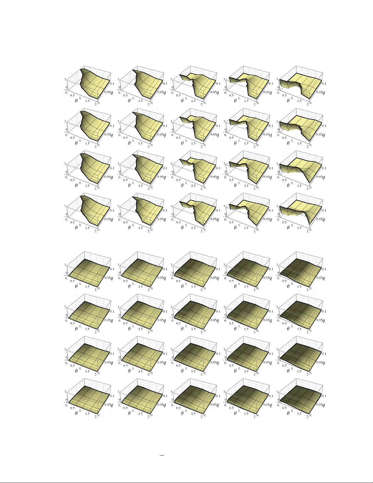
Extensi v e Large-Scale Study of Error in Samping-Based Distinct V alue Estimators for Databases ∗ V inay Deolalikar † Hernan Laf ﬁtte ‡ Abstract The problem of distinct v alue estimation has many applications. Being a critical component of query optimizers in databases, it also has high commer - cial impact. Many distinct v alue estimators ha ve been proposed, using v arious statistical approaches. Howe ver , characterizing the errors incurred by these es- timators is an open problem: existing analytical approaches are not powerful enough, and extensi ve empirical studies at large scale do not exist. W e con- duct an extensi ve lar ge-scale empirical study of 11 distinct value estimators from four different approaches to the problem o ver families of Zipﬁan distri- butions whose parameters model real-world applications. Our study is the ﬁrst that scales to the size of a billion-r ows that today’ s lar ge commercial databases hav e to operate in. This allows us to characterize the error that is encountered in real-world applications of distinct value estimation. By mining the gener- ated data, we show that estimator error depends on a key latent parameter — the average uniform class size — that has not been studied previously . This parameter also allows us to unearth error patterns that were previously un- kno wn. Importantly , ours is the ﬁrst approach that provides a framew ork for ∗ This is the full-length v ersion of a shorter published paper , and includes supplementary material for the published paper . Please cite as “V inay Deolalikar and Hernan Lafﬁtte: Extensi ve Large- Scale Study of Error in Samping-Based Distinct V alue Estimators for Databases, IEEE Big Data Conference, W ashington DC, December 2016. ” † contact author , deolalikar.academic@gmail.com , work done at HP Labs, Palo Alto. ‡ hernan.laffitte@hp.com 1 visualizing the err or patterns in distinct value estimation, facilitating discus- sion of this problem in enterprise settings. Our characterization of errors can be used for se veral problems in distinct v alue estimation, such as the design of hybrid estimators. This work aims at the practitioner and the researcher alike, and addresses questions frequently asked by both audiences. 1 Intr oduction Consider the following problem: estimate the number of distinct v alues (or classes) in a population by statistically analyzing its sample. This is the problem of distinct value estimation , and it arises in a surprisingly large variety of applications, where it is used to estimate a number of interest: in census studies, the number of indi vid- uals in lists having duplications [20]; in economics, the number of inv estors from samples of share registers of companies [23]; in ecology , the number of species from some sampling scheme [29]; in numismatics, the number of coins produced by a mint when a selection of such coins has been found [7]. Ho wev er , the application that has arguably the most commercial impact arises in databases 1 . Large data warehouses rely on complex query optimizers to formulate their query plans. A query optimizer needs an estimate of the number of distinct v alues in its attributes in order to formulate its query plan [19]. On attributes that are not inde xed, single pass (or scan) estimators provide fairly accurate estimates of dis- tinct v alues while using a small memory footprint [14, 2]. Ho wev er, databases ha ve witnessed explosi ve gro wth over the past decade; today’ s large commercial data warehouses have billions of ro ws. Therefore, accessing all the data in this manner is seldom possible. This makes sampling based estimators of distinct values the only practical solution for distinct v alue estimation. All the large scale commercial databases that we are aw are of use sampling based estimators of distinct values as part of their query optimizer . A great range of sampling based estimators for distinct values hav e been pro- posed in both the statistics and database literature, see [3] for a survey . Distinct v alue estimation is a hard problem, and estimators generally incur (signiﬁcant) er- rors in performing the estimates. Therefore, users with some kno wledge about the 1 The high-end large data w arehouse market for 2022 is estimated to be $22B [30]. 2 datasets they will encounter in applications, are interested in the following ques- tions. Q1 From this plethora of distinct value estimators, which estimator will giv e the least error on their dataset which is of the size of a typical database — (mil- lions to a billion ro ws)? Q2 For a choice of estimator , can one characterize the errors that will be incurred on such a large dataset? Q3 Ho w high should the sampling fraction be in order to keep error within a tolerable margin? Con versely , giv en a sampling fraction and a desired error margin, what choice of estimator will restrict errors to that mar gin? Q4 Do the errors occur in patterns that can be ef fectiv ely visualized? These problems ha ve serious practical ramiﬁcations in database design: a poor estimate of distinct values can result in a considerably more expensi ve query plan [19]. Furthermore, a query estimator may ha ve more tolerance for a certain region of bias, as opposed to other regions (depending on the region where the query plan changes from a good one to an inefﬁcient one). Unfortunately , due to the difﬁculty of the problem, and the lack of an adequate characterization of errors, commercial systems often suffer from unexpected poor estimates that seem to occur “at ran- dom”. These cause the query optimizer to formulate highly inefﬁcient query plans, resulting in intolerable delays to the system user , especially when the database has in excess of hundred million ro ws. Simply put, our state of knowledge about error in distinct v alue estimators is untenable due to the large sizes of today’ s databases. One might think that a way out would be to increase the sampling fraction. Ho wev er , the cost of ev en 1% sampling in a commercial database with billions of ro ws, is signiﬁcant, and a larger than 2% sample is often simply not possible. Also, because data is stored in blocks, generating a 10% random sample is sometimes as expensi ve as scanning all the data. Therefore, there is great practical interest in the least sample size that can deli ver a reasonable estimate of distinct v alues. Finally , visual descriptions of errors, in addition to facilitating one’ s own under- standing, permit effecti ve communication to non-specialists, which is an important aspect of working with statistical technologies in an enterprise setting. 3 Unfortunately , there do not yet exist analytical techniques that characterize er- ror satisfactorily (or answer any of (Q1)-(Q4)) for any distinct value estimator in literature (except, to a degree, for the ˆ D GEE , see 2). Instead, there is a powerful result in the “opposite direction” in [10, 9] that says that ev ery estimator will give a large error on some dataset. This suggests that new analytical approaches may ha ve to be de veloped for speciﬁc datasets/distributions. In the absence of analytical approaches to characterizing error , we must turn to empirical characterizations performed through a lar ge-scale extensi ve study ov er distributions that represent real-world applications. Howe ver , here, the situation is best described by [19]: “Unfortunately , analysis of distinct value estimators is non-tri vial, and few analytic results are av ailable. T o make matters worse, there has been no ex- tensi ve empirical testing or comparison of estimators either in the database or statistical literature...the testing that has been done in the statistical literature has generally in volv ed small sets of data in which the frequencies of different attribute v alues are fairly uniform; real data is seldom so well-beha ved. ” The impetus for our work arose from an effort, during the year 2007, to de- sign a distinct v alue estimator for a large commercial HP database product that had, among its customers, a F ortune-10 compan y . At that time, we did not ﬁnd an exten- si ve, large-scale, comparati ve study on distinct value estimators that would allo w us to answer questions (Q1)-(Q4) reliably for critical database applications. Sev eral studies in literature showed dif ferent estimators to be the best ov er the datasets in the purview of the particular study . These are valuable data points, b ut the y are al- most ne ver comparable, and it is not clear ho w far the results generalize (see § 2.2). This is the gap that the current paper aims to ﬁll. This brings us to our approach. Our study characterizes error in distinct value estimators, and provides answers to (Q1)-(Q4). Our approach can be described in the follo wing steps. 1. Conduct an extensi ve empirical study of the relative performance of various estimators on a well-chosen parameter space . 4 2. Mine the generated data for stable patterns to the relati ve performance of estimators on datasets, 3. Find parameters that org anize these stable patterns. 4. Present these stable patterns in a manner that is easy to visualize and commu- nicate among practitioners. 5. Characterize error through bias, ratio-error , and RMSE, for each re gion of the parameter space that is delineated by stable patterns of behavior . 1.1 Our Contributions Our e xtensiv e empirical study allowed us to construct a detailed large-scale charac- terization of the relativ e behavior of important families of distinct v alue estimators. Our study is the ﬁrst that scales to the billion-ro w size that today’ s large commercial databases operate on. Our characterization describes both inter - and intra-family be- havior over a parameter space that models the variation of real-world data. W e iden- tify stable patterns of beha vior that allo w us to “make sense” of the huge amount of data generated in our empirical study . W e identify a critical latent parameter — the av erage uniform class size — that estimators are sensitiv e to, and that allows us to ﬁnd patterns in our results. This variable has not yet been studied in literature. Our study allo ws us to answer the following types of questions. 1. What are scale ef fects on each estimator? 2. What are ske wness effects on each estimator? 3. Ho w does the actual distinct value count af fect an estimator? 4. What is the “best” estimator under v arious deﬁnitions? 5. What sampling percentage is adequate for v arious error requirements? Finally , our study allo ws us to comparati vely e v aluate, at large-scale, the four dif ferent approaches to distinct value estimation that are within our purvie w . Limitations and Scope of our Study . Our study is most useful for distributions that approximate a po wer law , and with population parameters that resemble those of our study . Ho we ver , both these are intended to reﬂect real-world problems. 5 2 Related W ork Over the years, a gro wing number of methods have been used to construct estima- tors for the distinct v alues problem [3]. As pointed out by [20], there are fe w papers that focus on the case where the population size is kno wn. This is the case that models applications to databases. First, we brieﬂy survey results on unsuitability of se veral proposed estimators for large scale applications. These include the earli- est distinct v alue estimators from statistics that were used for database applications [21, 25]. • The estimators ˆ D Goo d1 and ˆ D Goo d2 from [17] are unbiased, but ha ve ex- tremely high v ariance, and are numerically unstable at small sample sizes [21, 24, 19, 3]. • The estimator ˆ D Chao from [25, 6] underestimates, except where f 2 = 0 , where it blo ws up [19]. • The jacknife estimator ˆ D CJ [25] based on [4, 5] is deriv ed from inapplicable assumptions [19]. • The estimator ˆ D Sichel [28] is unsuitable since the two-parameter GIGP does not ﬁt se veral datasets [19]. • The method of moments estimators ˆ D MM0 , ˆ D MM1 , and ˆ D MM2 [19] yield poor estimates when γ 2 > 1 [19]. • ˆ D Boot [29] has the property that ˆ D Boot < 2 d , therefore poor performance is likely at lar ge D and small q [19]. 2.1 The Estimators Under Study The 11 estimators that are selected for our study come four different approaches to distinct value estimation, and have been proposed as being suitable for the scale of database applications. W e set notation before we commence their description. Consider a population of size N that has D classes of sizes N 1 , . . . , N D so that N = P D j =1 N j . W e denote by F i the number of classes of size i in the population, so that D = P N i =1 F i . Samples of size n = q N may be drawn from the population. Here q is the sampling fraction. The resulting sample has d classes (therefore d ≤ D ). W e denote by f i the number of classes in the sample that occur i times, so that 6 T able 1: Notation Symbol Meaning Notes N size of population very lar ge (millions to billion) D number of classes in population quantity to be estimated N j size of j th class in population P N j = N ¯ N av erage class size in population ¯ N = N /D γ 2 squared coefﬁcient of v ariation of class sizes γ 2 = (1 /D )( P D j =1 ( N j − ¯ N ) 2 ) / ( ¯ N ) 2 F i number of classes of size i in the population D = P F i , N = P iF i n size of sample drawn from population preferably small q sampling fraction q = n/ N n j size of j th class in sample may be zero d distinct classes in sample number of non-zero n j f i number of classes of size i in the sample d = P f i , n = P if i ˆ D estimator for D subscripts indicate different estimators θ sk e wness parameter for a Zipﬁan population deﬁned in § 3 A size of alphabet for Zipﬁan population deﬁned in § 3 N A av erage uniform class size deﬁned in § 3 d = P n i =1 f i and P n i =1 if i = n . W e wish to form an estimate ˆ D of D by analyzing the sample, and using the kno wn value N . For con venience, we place the notation deﬁned earlier , as well as that to be deﬁned shortly , in T able 1. No w we come to the estimators in our study . W e will ﬁnd it con venient to describe the remaining estimators with the model ˆ D = d + f 0 , (1) where f 0 is the number of classes that are not represented in the sample. The ﬁrst estimator is proposed by [27] who consider the task of b uilding estimators for dic- tionaries. The estimators constructed assume that the population size is large, the sampling fraction is non-negligible, and that the proportions of classes in the sam- ple reﬂects that in the population, namely E [ f i ] E [ f 1 ] = F i F 1 . Under these assumptions, 7 Schlosser deri ved the estimator ˆ D Sh = d + f 1 P n i =1 (1 − q ) i f i P n i =1 iq (1 − q ) i − 1 f i . Note that the estimate of classes not represented in the sample is a function of f 1 . This estimator w as constructed for language dictionaries, and w ord usage is kno wn to be Zipﬁan with a high ske wness parameter , and the assumptions are indeed valid in the application under study . The next family of estimators is from [20], and uses the bias reducing jackknif- ing technique of [18]. It is of the form ˆ D = d + K f 1 n . (2) Namely , the jackknife estimate of f 0 is K f 1 /n . Using ﬁrst and second order meth- ods, [20] deri ve dif ferent values of the parameter K , resulting in the estimators ˆ D uj1 and ˆ D uj2 , respectiv ely . The second order estimator ˆ D uj2 requires estimation of the squared coefﬁcient of variation γ 2 = (1 /D )( P D j =1 ( N j − ¯ N ) 2 ) / ¯ N 2 , where ¯ N = N/D . A method of moments estimate based on ˆ D is used as follo ws ˆ γ 2 ( ˆ D ) = max 0 , ˆ D n 2 n X i =1 i ( i − 1) f i + ˆ D N − 1 ! . (3) They then construct an estimator that “smooths” the second order estimator , resulting in ˆ D sj2 . These estimators are given belo w . ˆ D uj1 =  1 − (1 − q ) f 1 n  − 1 d, (4) ˆ D uj2 =  1 − (1 − q ) f 1 n  − 1 d − f 1 (1 − q ) ln(1 − q ) ˆ γ 2 ( ˆ D uj1 ) q ! , (5) ˆ D sj2 =(1 − (1 − q ) ˜ N ) − 1 ( d − (1 − q ) ˜ N ln(1 − q ) N ˆ γ 2 ( ˆ D uj1 )) , (6) where ˜ N is an estimate of the av erage class size, and is set to N / ˆ D uj1 . Finally , they use a “stabilizing” technique from [8] to construct the estimator ˆ D uj2a as fol- 8 lo ws. Fix c > 1 and remov e all classes whose frequency in the sample exceeds c . Then compute ˆ D uj2 of the reduced sample, and increment it by the number of the pre viously removed classes, gi ving ˆ D uj2a . In our experiments, we used c = 50 . [20] then observe that the estimator ˆ D Sh also conforms to the model (1) with parameter K = K Sh = n P n i =1 (1 − q ) i f i P n i =1 iq (1 − q ) i − 1 f i . Replacing K Sh with alternativ e expressions, they obtain the following two esti- mators. ˆ D Sh2 = d + f 1 q (1 + q ) ˜ N − 1 (1 + q ) ˜ N − 1 !  P n i =1 (1 − q ) i f i P n i =1 iq (1 − q ) i − 1 f i  , (7) ˆ D Sh3 = d + f 1  P n i =1 iq 2 (1 − q 2 ) i − 1 f i P n i =1 (1 − q ) i ((1 + q ) i − 1) f i   P n i =1 (1 − q ) i f i P n i =1 iq (1 − q ) i − 1 f i  . (8) W e encountered ﬂoating point errors when ev aluating ˆ D Sh2 for large N , and so approximated the term in the ﬁrst parentheses in (7) by q / (1 + q ) in those cases. In another stream of research [10, 9] reason that classes that occur frequently in the sample represent a single class in the population. Ho wev er , classes that occur infrequently could represent multiple classes in the population. By estimating how many classes each such infrequent class represents, they construct two estimators: ˆ D GEE [10] and ˆ D AE [9], a heuristic estimator that adapts to the distribution sk ew . ˆ D GEE = r N n f 1 + n X j =2 f j , (9) ˆ D AE = d + K f 1 , where (10) K = P n i =3 e − i f i + me ( f 1 +2 f 2 ) /m P n i =3 ie − i f i + ( f 1 + 2 f 2 ) e − ( f 1 +2 f 2 ) /m . (11) T o solve for m abov e, we use m − f 1 − f 2 = K f 1 . Notice that ˆ D GEE conforms to (1) with f 0 = ( q N n − 1) f 1 . The ne xt approach to distinct value es timation e valuated in our study is through the notion of “sample cov erage”. Sample cov erage C is deﬁned as the fraction of 9 classes in the population that appears in the sample. This approach was proposed by T uring [15], who suggested the follo wing estimator of sample coverage. ˆ C = 1 − f 1 /n. Therefore, an estimate of the distinct v alues would be ˆ D 1 = d/ ˆ C . (12) [11] show that the abov e estimate is quite efﬁcient relati ve to the MLE of the same quantity . Further dev elopment of the sample cov erage method includes [16, 26, 12, 13]. The estimators we use are constructed in [7], and are “second order” in the sense that they require an estimate of the coefﬁcient of v ariation of the class distribution to correct the estimate (12) that holds for uniformly distributed classes. T wo estimators of γ 2 are constructed. ˜ γ 2 = max " ˆ D 1 P i ( i − 1) f i n 2 − n − 1 , 0 # , (13) ˆ γ 2 = max " ˜ γ 2 1 + n (1 − ˆ C ) P i ( i − 1) f i n ( n − 1) ˆ C ! , 0 # . (14) The abov e estimates of γ 2 result in the follo wing two estimators of D . ˆ D CL1 = d ˆ C + n (1 − ˆ C ) ˆ C ˜ γ 2 , (15) ˆ D CL2 = d ˆ C + n (1 − ˆ C ) ˆ C ˆ γ 2 . (16) These estimators are for a multinomial sampling regime (sampling with replace- ment) for an inﬁnite population. Howe ver , giv en the lar ge populations that we consider in our work, the adjustment for sampling without replacement from ﬁnite populations is negligible, and therefore conceiv ably these estimators could be used for the distinct v alue problem in databases as well. The aforementioned works pro vide strong theoretical contributions, and giv e us 10 a range of estimators, from dif ferent approaches to the distinct value problem. 2.2 Deﬁciencies in Empirical Studies W e note the follo wing types of deﬁciencies in previous studies. 1. The scale of the study is far too small and does not reﬂect today’ s commercial databases that handle billions of ro ws. 2. The studies in volv e too few datasets for stable patterns to emerge, so no generalized conclusions can be drawn. 3. The variation in parameters is over a signiﬁcantly smaller range than occurs in real-world applications. 4. Most studies report the RMSE, not the individual biases of each estimator . 5. Most studies do not consider sampling percentages lo wer than 1%, (most as- sume sampling percentages abov e 5%). In real world commercial data w arehouses, e ven 1% sampling is expensi ve, and one would lik e to make do with less. 6. Comparisons are made between members of one or two approaches to dis- tinct v alue estimation only . 7. Individual estimators are compared to hybrid estimators. 8. Differing notions of sk ewness, that are not proxies for each other , are used. 3 Methodology 3.1 Desiderata of Study Our empirical study was designed with the follo wing high-lev el desiderata. 1. W e wish to standardize our benchmarking setup so that in the future, differ - ent estimators can be systematically compared. 2. W e want to understand the behavior of estimators as an absolute function of parameters that are entirely in our control. 3. The parameter space should model real-world data. Characteristics of real-world data are numerous, and often interacting. W e can ne ver be certain which characteristic of the data is causing or inﬂuencing the per- formance of the estimator . In this way , the performance of the estimator becomes r elative , and not absolute as a function of a chosen set of parameters. 11 This points us to the use of artiﬁcially generated data from a well-chosen pa- rameter space, as the means to our desired characterization. The potential hazard in doing so is that the artiﬁcial data may not represent any real-world application. So while desiderata (1) and (2) are met, we might fail on (3). Recall that the family of Zipﬁan distributions Z A,θ parametrized by their ske w- ness parameter θ , and the size of the alphabet A , have probability masses P A,θ ( i ) satisfying P A,θ ( i ) ∝ 1 i θ . Normalizing so that we get a distribution, we obtain the probability mass P A,θ ( i ) = D X i =0 1 i θ ! − 1 1 i θ . It is by now accepted that sev eral naturally occurring distrib utions of importance are power laws, see [22] for div erse examples. Equally importantly , se veral distri- butions approximate po wer la ws once their outliers are remo ved. Sev eral quantities stored in our commercial database systems also follo w po wer law distributions af- ter similar processing. Therefore, a study on a Zipﬁan parameter space is important in and of itself. Secondly , the Zipﬁan distribution allows us to vary just the right parameters — namely ske wness and the size of the unique alphabet — that are most germane to the performance of distinct v alue estimators. In light of the discussion abov e, we choose to characterize our estimators over a Zipﬁan parameter space, by v arying the parameters of the Zipﬁan population over a wide range of values that reﬂect real-world applications. In this way , we get the “best of both worlds” — we are able to v ary parameters, understand estimator behavior as an absolute function of these parameters, and model real-world appli- cations. 3.2 Datasets and Protocol In order to obtain a ﬁne grained characterization, we use the design of (population size, alphabet size) pairs as shown in T able 2. Each such pair will be called a r e gime . Therefore, there are 20 regimes. As depicted, the regimes were organized into ﬁve N A v alues in [10 , 20 , 100 , 500 , 1000] . For each regime, we generated 5 Zipﬁan populations by v arying the Zipﬁan ske wness parameter θ through the range [0 , 0 . 5 , 1 , 1 . 5 , 2] that covers most real- 12 T able 2: The (population size, alphabet size) regimes used to generate Zipﬁan populations. This table also indicates the lay out of the grid on which the 2D normalized bias plots and 3D nor - malized bias surfaces are laid thr oughout the paper . 1 B , 100 M 1 B , 50 M 1 B , 10 M 1 B , 5 M 1 B , 1 M N → 100 M , 10 M 100 M , 5 M 100 M , 1 M 100 M , 500 K 100 M , 100 K 10 M , 1 M 10 M , 500 K 10 M , 100 K 10 M , 50 K 10 M , 10 K 1 M , 100 K 1 M , 50 K 1 M , 10 K 1 M , 5 K 1 M , 1 K N A → world applications. In this way , we obtain 100 Zipﬁan populations. Note that at high skewness, the number of distinct classes D in the population is less than the size of the alphabet A . W e refer to N A as the aver age uniform class size since it is the a verage class size when θ = 0 (and up till the time that each alphabet occurs in the population). W e will see that it is a critical parameter in characterizing estimator error . For each of the 100 Zipﬁan populations, we v aried the sampling percentage through the v alues [0 . 1 , 1 , 2 , 5 , 10] . F or each data-point, we drew 10 random sam- ples without replacement. W e ran our 11 distinct v alue estimators on each of the 10 samples, thereby generating 10 estimates for each of the 11 estimators. Fi- nally , for each estimator , we computed the av erage bias of the 10 estimates, as well as the variance across the 10 estimates. In this way , we report a total of 100 × 5 × 10 × 11 = 55 , 000 experiments. W e should note that in our study , we experimented with a strictly larger range of parameter values than what is reported in this paper . Ho wev er , to conserve space, we “compress” to a subset of our range of parameter v alues that we feel adequately described the error patterns. 4 Results Our extensi ve empirical study generated a large amount of data. Our goal is to provide a thorough characterization of both, the individual and relati ve performance of the estimators, and to organize and understand the error patterns that emerged from our study . By mining the generated data, we found that the parameter N A provides us with this organizing principle: when the results of the experiments ar e arrang ed in a grid whose X-axis is N A , and Y -axis is N , we can see r e gularity in the 13 patterns . Accordingly , we provide grids of 2D plots of estimate vs. actual distincts for all estimators in a family , as well as grids of 3D surfaces showing normalized bias ( ˆ D − D ) /D for each individual estimator . In both cases v arying the parameters of the underlying population as well as the sampling fraction. For the 3D surfaces, normalized biases of -1, 0, and 3 are marked on the vertical axes, and 1 and 2 can be seen in the form of dotted lines. W e then point out the salient features of both the relati ve and the indi vidual behaviors as we v ary the parameters of the population. W e observe patterns that arise when we go from left to right on each row of the 2D plots. This giv es us the v ariations with the parameter N A . Like wise, we report variations with N , within each plot with θ , and, ﬁnally , with q . T o sa ve space, we sho w only a single 2D plot for each family: the one at which the maximum ratio error for the most accurate estimator in the family is at most 5 (T able 6). The remaining 2D plots are all included in supplementary material. W e suggest that when reading the results, the reader be gin with the 3D surfaces for each estimator to understand its indi vidual performance, followed by inspection of the 2D plots (including those in the supplementaries) to complete the relati ve picture. Note that putting multiple 3D surfaces into a single diagram is not feasible. W e be gin with the jackknife family . 4.1 The Jackknife Estimators V ariation with N A : ˆ D uj1 is fairly agnostic to changes in N A , at all values of q . On the other hand, the positiv e bias of ˆ D uj2 shoots up as N A increases. The magnitude of the positi ve bias is highest at mid-ske w . For ˆ D sj2 , the bias 3D surface illustrates best the sev ere positi ve bias at mid- ske w . Importantly , the bias magnitude, as also the region, reduces as N A increases. In other words, smoothing is more ef fective as N A increases. At N A = 10 , we need considerably ov er 10% sampling to get accurate estimates. As N A increases, the least sampling fraction q required to get accurate estimates reduces. The stabilized estimator ˆ D uj2a is quite accurate ov erall. There is a jump between lo w and high ske w estimates that increases with N A when q < 0 . 05 . There is a b ump at mid-ske w for low q and high N A ; it ﬂattens out at lo wer N A . 14 (a) Grid of 3D bias surfaces for ˆ D uj1 . (b) Grid of 3D bias surfaces for ˆ D uj2 . Figure 1: Notice that ˆ D uj1 is a consistent under -estimator of distinct values. Although second order , ˆ D uj2 has considerably worse and irregular bias beha vior as compared to ˆ D uj1 . Recall that the layout of the surfaces is on the grid indicated by T able 2. N A = 10 N A = 20 N A = 100 N A = 200 N A = 1000 N = 1B ç ç ç ç ç ´ ´ ´ ´ ø ø ø ø æ æ æ æ æ 0.5 1 1.5 2 Θ 0 A 2A A = 100M ç ç ç ç ç ´ ´ ´ ´ ø ø ø ø æ æ æ æ æ 0.5 1 1.5 2 Θ 0 A 2A A = 50M ç ç ç ç ç ´ ´ ´ ´ ø ø ø ø æ æ æ æ æ 0.5 1 1.5 2 Θ 0 A 2A A = 10M ç ç ç ç ç ´ ´ ´ ´ ø ø ø ø æ æ æ æ æ 0.5 1 1.5 2 Θ 0 A 2A A = 5M ç ç ç ç ç ´ ´ ´ ´ ø ø ø ø ø æ æ æ æ æ 0.5 1 1.5 2 Θ 0 A 2A A = 1M N = 100M ç ç ç ç ç ´ ´ ´ ´ ø ø ø ø æ æ æ æ æ 0.5 1 1.5 2 Θ 0 A 2A A = 10M ç ç ç ç ç ´ ´ ´ ´ ø ø ø ø æ æ æ æ æ 0.5 1 1.5 2 Θ 0 A 2A A = 5M ç ç ç ç ç ´ ´ ´ ´ ø ø ø ø æ æ æ æ æ 0.5 1 1.5 2 Θ 0 A 2A A = 1M ç ç ç ç ç ´ ´ ´ ´ ø ø ø ø æ æ æ æ æ 0.5 1 1.5 2 Θ 0 A 2A A = 500K ç ç ç ç ç ´ ´ ´ ø ø ø ø ø æ æ æ æ æ 0.5 1 1.5 2 Θ 0 A 2A A = 100K N = 10M ç ç ç ç ç ´ ´ ´ ´ ø ø ø ø æ æ æ æ æ 0.5 1 1.5 2 Θ 0 A 2A A = 1M ç ç ç ç ç ´ ´ ´ ø ø ø ø æ æ æ æ æ 0.5 1 1.5 2 Θ 0 A 2A A = 500K ç ç ç ç ç ´ ´ ´ ø ø ø ø æ æ æ æ æ 0.5 1 1.5 2 Θ 0 A 2A A = 100K ç ç ç ç ç ´ ´ ´ ø ø ø ø æ æ æ æ æ 0.5 1 1.5 2 Θ 0 A 2A A = 50K ç ç ç ç ç ´ ´ ´ ø ø ø ø ø æ æ æ æ æ 0.5 1 1.5 2 Θ 0 A 2A A = 10K N = 1M ç ç ç ç ç ´ ´ ´ ´ ø ø ø ø æ æ æ æ æ 0.5 1 1.5 2 Θ 0 A 2A A = 100K ç ç ç ç ç ´ ´ ´ ´ ø ø ø ø æ æ æ æ æ 0.5 1 1.5 2 Θ 0 A 2A A = 50K ç ç ç ç ç ´ ´ ´ ø ø ø ø æ æ æ æ æ 0.5 1 1.5 2 Θ 0 A 2A A = 10K ç ç ç ç ç ´ ´ ´ ø ø ø ø æ æ æ æ æ 0.5 1 1.5 2 Θ 0 A 2A A = 5K ç ç ç ç ç ´ ´ ø ø ø ø ø æ æ æ æ æ 0.5 1 1.5 2 Θ 0 A 2A A = 1K Jackknife family at q = 0.01 Distincts: D ` uj1 : ç D ` uj2 : ´ D ` sj2 : ø D ` uj2a : æ Figure 2: Relative behavior of the jackknife family at q = 0 . 01 , which is the lowest q at which ˆ D uj2a has a maximum error-ratio of 5 (see T able 6). Note the consistent underestimation of ˆ D uj1 , severe mid-ske w biases of ˆ D uj2 and ˆ D sj2 , and effect of stabilization in ˆ D uj2a . V ariation with N keeping N A ﬁxed: ˆ D uj1 is fairly agnostic of N . On the other hand, the accuracy of ˆ D uj2 at high ske w varies with N : ˆ D uj2 is more accurate at high ske w at high N , and inaccurate at low N . ˆ D sj2 is slightly worse at mid-ske w as N increases. Finally , ˆ D uj2a is fairly agnostic to N . V ariation with θ : As is known [3], ˆ D uj1 is a consistent underestimator across all θ . W e observe that the ne gati ve bias is the worst at mid-high sk e w . The bias proﬁle of ˆ D uj2 is best described as “hat-shaped”. There is se vere positiv e bias at mid- ske w . There is slight positi ve bias at lo w-skew , and moderate to high positi ve bias at high-ske w up to N = 100 M . At N > 100 M , ˆ D uj2 becomes an underestimator at high-ske w . The positi ve bias at high-ske w for lo w N gets worse as we increase q . ˆ D sj2 sho ws the same pattern of positiv e bias as ˆ D uj2 , but less prominently o wing to the smoothing. Smoothing also delays the poor performance at high N A . ˆ D uj2a has a crossov er in the form of a reﬂected “S” shape as we increase skew . In other words, it overestimates at mid ske w and underestimates at high ske w . See 16 also Fig. 8. At high N A , the bias goes from positi ve to negati ve as skew increases, whereas at lo w N A , it remains largely positi ve, with some o verestimation at high q . V ariation with q : As we might expect, ˆ D uj1 reduces its negati ve bias as q in- creases. ˆ D uj2 , at high N A , improv es dramatically in mid-ske w as q increases above 5%. Whereas, at low N A , increasing q does not help. For ˆ D sj2 increasing q helps more at high N A (100 or greater). F or N A = 100 , we need q > 10% , for N A = 200 this drops to q > 5% , and for N A = 1000 , we need only q > 1% for acceptable estimates. ˆ D uj2a does well at all sampling fractions and improves accuracy with q . At high Zipﬁan ske w of θ ≥ 1 . 5 , we need only q ≥ 0 . 005 for accurate estimates. Anomalies: The bias of ˆ D uj2 is lower at q = 0 . 001 as compared to higher values of q in the vicinity . The smoothing technique of ˆ D sj2 does well at lo w N A ∼ 10 , and very lo w sampling ( q = 0.001), but then exhibits poor performance as either of these parameters increases. 4.2 The Schlosser Estimators Bias: The Schlossers hav e the general bias proﬁle ˆ D Sh > ˆ D Sh3 > D > ˆ D Sh2 : the exception being at low N A and low q where ˆ D Sh and ˆ D Sh3 underestimate, but only slightly . V ariation with N A : For ˆ D Sh and ˆ D Sh3 , the bias curve is a slope at lower N A and becomes a “hat” at higher N A . The v alue of N A at which this shape transition happens reduces as q increases. For q = 0 . 001 , it happens after N A > 1000 , at q = 0 . 005 , it happens for N A between 1000 and 200, and for q = 0 . 02 , it occurs for N A between 200 and 100. Increase in q improv es accuracy as N A increases, with this improv ement manifesting at lo w skewness. ˆ D Sh3 is reasonably accurate at q ≥ 0 . 005 . ˆ D Sh requires q ≥ 0 . 01 for acceptable estimates. As q increases, the N A at which the accuracy is attained for low ske w reduces, and the range of low-sk ew where the accuracy is attained also increases. For lo w N A ∼ 10 , low ske w estimates remain intolerably poor until we raise the sampling fraction to q = 0 . 1 . The predominant effect of increasing N A on all three is that the lower ske w esti- mate becomes reasonably accurate. See also Fig. 8 for this effect in ˆ D Sh2 . 17 (a) Grid of 3D bias surfaces for ˆ D sj2 (b) Grid of 3D bias surfaces for ˆ D uj2a Figure 3: Effect of smoothing versus stabilization can be seen clearly: the stabilized ˆ D uj2a is one of the most consistently accurate estimators, while the smoothed ˆ D sj2 is suffers severe mid-ske w bias at low N A . Note the ef fect of N A versus that of N in ˆ D sj2 . (a) Grid of 3D bias surfaces for ˆ D Sh (b) Grid of 3D bias surfaces for ˆ D Sh2 Figure 4: ˆ D Sh shows severe positive bias at lower skew , that is corrected only with high sampling fractions. ˆ D Sh2 does not suffer from this problem. Note the highly regular behavior of both, espe- cially clear with ˆ D Sh , as a function of N A alone. V ariation with N : There is little change in the shape of the bias surfaces as we increase N , keeping N A ﬁxed. Figure 5: Grid of 3D bias surface for ˆ D Sh3 . Like ˆ D Sh , there is severe positi ve bias at low ske w . Note again the highly regular beha vior of ˆ D Sh3 as a function of N A alone. V ariation with θ : ˆ D Sh and ˆ D Sh3 are extremely accurate for high-skew . When the bias curve becomes a hat, as described earlier , the estimator is accurate at low ske w also (pl. see v ariation with N A for discussion of when it becomes a hat). When this happens, only mid-ske w is overestimated. ˆ D Sh2 has a negati ve bias at low-mid ske w , but is not as extreme as ˆ D Sh and ˆ D Sh3 . V ariation with q : This family is very sensitiv e to q , and shows monotonic im- prov ement in accuracy (which means lesser positi ve bias) as q increases. In the range of 5 - 10% sampling, all three estimators begin giving accurate estimates for all N A , all ske w , and all N , gi ving a maximum ratio error of ∼ 5 . Of these, ˆ D Sh3 is requires the lowest q to provide acceptable estimates across the range of ske w (see T able 6. 20 N A = 10 N A = 20 N A = 100 N A = 200 N A = 1000 N = 1B á á á ò ò ò ò ò ð ð ð 0.5 1 1.5 2 Θ 0 A 2A A = 100M á á á ò ò ò ò ò ð ð ð 0.5 1 1.5 2 Θ 0 A 2A A = 50M á á á á ò ò ò ò ò ð ð ð ð 0.5 1 1.5 2 Θ 0 A 2A A = 10M á á á á ò ò ò ò ò ð ð ð ð ð 0.5 1 1.5 2 Θ 0 A 2A A = 5M á á á á á ò ò ò ò ò ð ð ð ð ð 0.5 1 1.5 2 Θ 0 A 2A A = 1M N = 100M á á á ò ò ò ò ò ð ð ð 0.5 1 1.5 2 Θ 0 A 2A A = 10M á á á ò ò ò ò ò ð ð ð 0.5 1 1.5 2 Θ 0 A 2A A = 5M á á á á ò ò ò ò ò ð ð ð ð 0.5 1 1.5 2 Θ 0 A 2A A = 1M á á á á ò ò ò ò ò ð ð ð ð ð 0.5 1 1.5 2 Θ 0 A 2A A = 500K á á á á á ò ò ò ò ò ð ð ð ð ð 0.5 1 1.5 2 Θ 0 A 2A A = 100K N = 10M á á á ò ò ò ò ò ð ð ð 0.5 1 1.5 2 Θ 0 A 2A A = 1M á á á ò ò ò ò ò ð ð ð 0.5 1 1.5 2 Θ 0 A 2A A = 500K á á á á ò ò ò ò ò ð ð ð ð ð 0.5 1 1.5 2 Θ 0 A 2A A = 100K á á á á ò ò ò ò ò ð ð ð ð ð 0.5 1 1.5 2 Θ 0 A 2A A = 50K á á á á ò ò ò ò ò ð ð ð ð ð 0.5 1 1.5 2 Θ 0 A 2A A = 10K N = 1M á á á ò ò ò ò ò ð ð ð 0.5 1 1.5 2 Θ 0 A 2A A = 100K á á ò ò ò ò ò ð ð ð 0.5 1 1.5 2 Θ 0 A 2A A = 50K á á á á ò ò ò ò ò ð ð ð ð ð 0.5 1 1.5 2 Θ 0 A 2A A = 10K á á á á á ò ò ò ò ò ð ð ð ð ð 0.5 1 1.5 2 Θ 0 A 2A A = 5K á á á á á ò ò ò ò ò ð ð ð ð ð 0.5 1 1.5 2 Θ 0 A 2A A = 1K Schlosser family at q = 0.05 Distincts: D ` Sh : á D ` Sh2 : ò D ` Sh3 : ð Figure 6: Relati ve behavior of the Schlosser family at q = 0 . 05 , which is the lo west q at which ˆ D Sh2 has a maximum ratio-error of 5. Even at a relativ ely high sampling fraction, ˆ D Sh and ˆ D Sh3 show sev ere positi ve bias at low-mid skew . In order to use these estimators at low-mid skew , q ≥ 0 . 1 is required. 4.3 ˆ D GEE and ˆ D AE V ariation with N A : At lo w N A ∼ 10 , both ˆ D GEE and ˆ D AE underestimate but both are reasonably accurate. As we increase N A , this picture changes signiﬁcantly for ˆ D GEE , b ut not for ˆ D AE (see Fig. 7. ˆ D AE sho ws considerably less change w .r .t. N A . The change of ˆ D GEE with N A is described next. There is a change from a slope to a “hat”, similar to ˆ D Sh and ˆ D Sh3 , as N A rises. Ho wev er , the degree of ov erestimation is not comparable the Schlossers. The ratio errors for the worst case positiv e bias is less than 10, compared to over 200 for Schlossers. The transition to “hat” happens at q = 0 . 005 at N A between 1000 and 200; at q = 0 . 02 between 200 and 100; and at q = 0 . 1 between 100 and 20. V ariation with N : There is little change with N except for some reduction in positi ve bias for high-ske w for ˆ D GEE with N . 21 (a) Grid of 3D bias surface for ˆ D GEE (b) Grid of 3D bias surface for ˆ D AE Figure 7: ˆ D GEE and ˆ D AE are among the most consistent estimators. ˆ D GEE does have a re gion of positiv e bias at high N A , where it should not be used in preference to ˆ D AE and ˆ D uj2a . Both estimators show highly re gular behavior as a function of N A . V ariation with θ : ˆ D GEE is very good at high ske w . When the transition to “hat” shape happens, it becomes good at low skew as well (see previous discussion of when this happens). ˆ D GEE is a mid-ske w ov erestimator (except at very low q , where it underestimates). ˆ D AE is accurate at both high and low ske w Zipﬁan populations, with a tendency to wards ne gati ve bias. See also Fig. 8. Since both ˆ D GEE and ˆ D AE appear in the grid of 2D bias plots for the top three estimators in Sec 5, we do not sho w their 2D bias plots here. Of course, all the 2D bias plots are av ailable in the supplementaries. V ariation with q : Both estimators sho w monotonic improv ement in accuracy (re- duction in positiv e bias) for increase in q . For ˆ D GEE , at q = 0 . 005 worst case ratio error is 5, at q = 0 . 01 , it drops to 4, at q = 0 . 05 , it is less than 2. Anomalies: When changing N A from 20 to 100, there is a sudden increase in ˆ D GEE positi ve bias up to q = 0 . 01 . 4.4 The Chao-Lee Estimators The Chao-Lee estimators sho w highly erratic beha vior , and perform reasonably only in follo wing regions. 1. At q =0.001, N =1M, 10M 2. At q =0.005, N =10M 3. At q =0.001, N =100M 4. At q =0.5, N =1M and 100M 5. At q =0.1, N =10M The v ariations described below only pertain to the abo ve re gions. V ariation with N A : Not much change except at q = 0.001. V ariation with N : Discontinuity is the predominant effect. V ariation with θ and q : When q > 0 . 005 , both underestimate in mid-high ske w . 5 Discussion The discussion is organized as follows. First we describe the relati ve sensitivity of each estimator to the v arious parameters. Then we address the question “which are the best estimators?” in terms of accuracy over the entire parameter space of our characterization. Next, we identify regions of the parameter space where certain 23 (a) ˆ D uj1 (b) ˆ D uj2a (c) ˆ D Sh2 (d) ˆ D AE Figure 8: The “ﬂatter” bias surfaces of ˆ D uj1 , ˆ D uj2a , ˆ D Sh2 , and ˆ D AE shown with more detail. Only N = 1 B , and N A ∈ [10 , 100 , 1000] shown. Note also that these estimators are relatively agnostic to N , and show re gularity in variation with N A . Figure 9: The two Chao-Lee estimators show highly irregular behavior that becomes extreme even at N = 10 M . Therefore we show only 1M and 10M population sizes for ˆ D CL2 . The remaining 3D surfaces for ˆ D CL2 are av ailable in supplementaries. estimators do well, ev en though the y may not perform well ov er the entire parameter space. Finally , we address the question “ho w much sampling do we need?” 5.1 Sensitivity to Parameters Sensitivity to N A : The grids of 3D bias surfaces clearly sho w that e very f amily — the Schlossers, jackkniv es, ˆ D GEE and ˆ D AE , and Chao-Lee — is sensitive to changes in N A , and all except the last show regularity in their behaviour as a function of N A . The parameter N A emerges as the single most important organizing parameter for estimator beha vior ov erall. The sensitivity to N A is high in ˆ D Sh , ˆ D Sh3 , ˆ D uj2 , ˆ D sj2 , ˆ D GEE , ˆ D CL1 , and ˆ D CL2 . Compared to the above, there w as mild sensiti vity in ˆ D uj1 , ˆ D uj2a , ˆ D Sh2 , and ˆ D AE . Therefore, ev en within a family , some members are highly sensiti ve to changes in N A , while others are not. Sensitivity to Scale N : Among the 11 estimators we tested, ˆ D sj2 , and the two Chao-Lee estimators were highly sensiti ve to scale. Namely , as we go up v ertically along their grids, their 3D bias surfaces sho wed signiﬁcant changes. Of these, the change was quite regular and predictable in ˆ D sj2 , but irregular and unpredictable in the Chao-Lee families. In the case of ˆ D sj2 , the bias increases as we increase the scale, with the increase being most prominent around m id-ske w as can be seen from the 3D bias surf aces for ˆ D sj2 (Fig 3a). See supplementaries for complete Chao-Lee estimator grids. Sensitivity to Sampling Fraction q : The 2D plots (see supplementaries) are use- ful to illustrate the effect of sampling fraction. The estimators that impro ve most as q increases are ˆ D Sh , ˆ D Sh3 , ˆ D GEE . The estimators that are relativ ely less sensiti ve to increases in q in our range, for some v alues of other parameters, are ˆ D uj2a and ˆ D AE . For example, both of them remain relati vely accurate for low skew ev en at 25 lo w sampling fractions (see T ables 3 and 4). The estimators that sho w anomalous or irregular behavior as q is increased are ˆ D uj2 , ˆ D sj2 , and the Chao-Lee family . In the case of ˆ D uj2 and ˆ D sj2 , we see anomalous degradation in performance as we go from q = 0.001 to 0.005, especially when N A < 200 , see 2D plots in supplementaries. Sensitivity to Zifpian Skew θ : Sensiti vity to θ can be seen more ﬁnely in the 2D plots (see supplementaries). The estimators ˆ D Sh , ˆ D Sh3 , ˆ D uj2 , ˆ D sj2 , and ˆ D GEE are highly sensitiv e to changes in Zipﬁan ske w . In particular , ˆ D Sh and ˆ D Sh3 are quite inaccurate at low ske w . ˆ D uj2 and ˆ D sj2 perform poorly in mid-ske w , while ˆ D uj2 also performs poorly for smaller populations and high ske w , ev en at high sampling fractions. The estimators ˆ D Sh2 , ˆ D uj1 , ˆ D uj2a , and ˆ D AE are relati vely insensiti ve to changes in Zipﬁan skew . Finally , ˆ D CL1 and ˆ D CL2 respond irregularly to changes in Zifpian ske w . 5.2 The Best Estimators Overall and their Relativ e Perf ormance From our extensiv e study , we can conclude that three estimators provide relatively strong performance across variations in all underlying parameters. These three are ˆ D GEE , ˆ D AE , and ˆ D uj2a (cf. the choice of the provisional estimator in [3], which is ˆ D sj2 ). It is perhaps easiest to see this from T able 3, and inspect the low and high sampling cases separately . Of course, which estimator is to be used for an application depends on the sampling fraction that is av ailable (we return to this question in § . 5 . 5) , and the skewness of the population in case it is kno wn. A subtler issue is whether it is the ratio error that is critical to the application, or the actual v alue and sign of the bias, and the role played by N A . For example, when the number of distincts is relati vely low , even large ratio errors do not result in high absolute v alue of bias. Therefore, we cannot speak meaningfully about “best estimator” in terms of just ratio error or bias — we do need to include the N A factor as well. Since in certain database query optimizers, it may be the value and sign of bias that is the critical factor in change of a query plan, while in others, it may be the ratio error , practitioners will ﬁnd it useful to ha ve an analysis along both metrics. In both cases, we discuss the low sampling scenario ( q < 0 . 01 ) below since that is where 26 dif ferences may be most manifest. N A = 10 N A = 20 N A = 100 N A = 200 N A = 1000 N = 1B ´ ´ ´ ´ ´      æ æ æ æ æ 0.5 1 1.5 2 Θ 0 A 2A A = 100M ´ ´ ´ ´ ´      æ æ æ æ æ 0.5 1 1.5 2 Θ 0 A 2A A = 50M ´ ´ ´      æ æ æ æ æ 0.5 1 1.5 2 Θ 0 A 2A A = 10M ´ ´ ´ ´      æ æ æ æ æ 0.5 1 1.5 2 Θ 0 A 2A A = 5M ´ ´ ´ ´ ´      æ æ æ æ æ 0.5 1 1.5 2 Θ 0 A 2A A = 1M N = 100M ´ ´ ´ ´ ´      æ æ æ æ æ 0.5 1 1.5 2 Θ 0 A 2A A = 10M ´ ´ ´ ´ ´      æ æ æ æ æ 0.5 1 1.5 2 Θ 0 A 2A A = 5M ´ ´ ´      æ æ æ æ æ 0.5 1 1.5 2 Θ 0 A 2A A = 1M ´ ´ ´ ´      æ æ æ æ æ 0.5 1 1.5 2 Θ 0 A 2A A = 500K ´ ´ ´ ´ ´      æ æ æ æ æ 0.5 1 1.5 2 Θ 0 A 2A A = 100K N = 10M ´ ´ ´ ´ ´      æ æ æ æ æ 0.5 1 1.5 2 Θ 0 A 2A A = 1M ´ ´ ´ ´ ´      æ æ æ æ æ 0.5 1 1.5 2 Θ 0 A 2A A = 500K ´ ´ ´      æ æ æ æ æ 0.5 1 1.5 2 Θ 0 A 2A A = 100K ´ ´ ´ ´      æ æ æ æ æ 0.5 1 1.5 2 Θ 0 A 2A A = 50K ´ ´ ´ ´ ´      æ æ æ æ æ 0.5 1 1.5 2 Θ 0 A 2A A = 10K N = 1M ´ ´ ´ ´ ´      æ æ æ æ æ 0.5 1 1.5 2 Θ 0 A 2A A = 100K ´ ´ ´ ´ ´      æ æ æ æ æ 0.5 1 1.5 2 Θ 0 A 2A A = 50K ´ ´ ´      æ æ æ æ æ 0.5 1 1.5 2 Θ 0 A 2A A = 10K ´ ´ ´ ´      æ æ æ æ æ 0.5 1 1.5 2 Θ 0 A 2A A = 5K ´ ´ ´ ´ ´      æ æ æ æ æ 0.5 1 1.5 2 Θ 0 A 2A A = 1K Top performing at q = 0.02 Distincts: D ` GEE : ´ D ` AE :  D ` uj2a : æ Figure 10: The three most consistent estimators at q = 0 . 02 , which is the lowest q at which ˆ D AE has maximum ratio error at most 5, see T able 6 (although ˆ D uj2a offers the same at q = 0 . 01 ). Note that at mid-high N A there is a region of signiﬁcant lo w-mid skew bias for ˆ D GEE , described in text. 5.2.1 By Ratio Error See T able 3. For low sampling fractions, for low N A , ˆ D uj2a and ˆ D GEE are the best estimators when 0 ≤ θ ≤ 1 . For higher ske w , only ˆ D GEE continues to perform well. At high N A , and low-mid ske w , ˆ D uj2a and ˆ D AE are the best, which ˆ D GEE again does very well as N A increases. Cav eat: If N A is mid-high, and the data has lo w-mid sk ew , then ˆ D GEE should not be used unless the sampling fraction is greater than 0.01. 5.2.2 By Bias See T able 4. For low sampling fractions and for low N A , all three — ˆ D uj2a , ˆ D GEE , ˆ D AE — do well measured by bias. For high N A , for low-mid skew , ˆ D uj2a and ˆ D AE are the best estimators. As we raise ske w , ˆ D GEE is more accurate than both; howe ver , all three are good. 27 T able 3: Ratio-error vs. θ and N A , for lo w and high sampling fractions. Note that the high and low ranges for N A ov erlap on the mid-value of N A = 100 . 0 . 001 ≤ q ≤ 0 . 005 0 . 01 ≤ q ≤ 0 . 1 Ske w N A ˆ D uj1 ˆ D uj2 ˆ D sj2 ˆ D uj2a ˆ D uj1 ˆ D uj2 ˆ D sj2 ˆ D uj2a 0 ≤ θ ≤ 1 N A ≤ 100 12 . 99 8 . 24 3 . 33 2 . 43 2 . 69 28 . 23 4 . 16 1 . 23 1 . 5 ≤ θ ≤ 2 N A ≤ 100 38 . 56 5 . 8 38 . 69 9 . 24 8 . 06 8 . 88 8 . 14 2 . 07 0 ≤ θ ≤ 1 N A ≥ 100 3 . 04 19 . 89 3 . 46 1 . 28 1 . 22 19 . 26 1 . 63 1 . 13 1 . 5 ≤ θ ≤ 2 N A ≥ 100 27 . 8 6 . 57 28 . 5 7 . 21 6 . 23 9 . 46 6 . 27 1 . 83 0 . 001 ≤ q ≤ 0 . 005 0 . 01 ≤ q ≤ 0 . 1 Ske w N A ˆ D Sh ˆ D Sh2 ˆ D Sh3 ˆ D GEE ˆ D AE ˆ D Sh ˆ D Sh2 ˆ D Sh3 ˆ D GEE ˆ D AE 0 ≤ θ ≤ 1 N A ≤ 100 19 . 39 25 . 57 16 . 96 2 . 49 4 . 17 5 . 41 3 . 11 4 . 18 1 . 62 1 . 41 1 . 5 ≤ θ ≤ 2 N A ≤ 100 1 . 15 36 . 32 2 . 53 2 . 69 14 . 29 1 . 07 6 . 86 1 . 06 1 . 93 3 . 09 0 ≤ θ ≤ 1 N A ≥ 100 64 . 7 3 . 87 45 . 7 4 . 27 1 . 56 4 . 08 1 . 2 2 . 57 1 . 65 1 . 06 1 . 5 ≤ θ ≤ 2 N A ≥ 100 1 . 81 26 . 19 2 . 23 2 . 12 10 . 94 1 . 32 5 . 39 1 . 23 1 . 65 2 . 62 T able 4: Percentage bias vs. θ and N A for low and high sampling fractions. Shaded cells indicate a change in the sign of the bias in the individual v alues within that region. 0 . 001 ≤ q ≤ 0 . 005 0 . 01 ≤ q ≤ 0 . 1 Ske w N A ˆ D uj1 ˆ D uj2 ˆ D sj2 ˆ D uj2a ˆ D uj1 ˆ D uj2 ˆ D sj2 ˆ D uj2a 0 ≤ θ ≤ 1 N A ≤ 100 − 50 . 01 680 . 77 181 . 94 − 34 . 67 − 33 . 07 2 , 719 . 94 310 . 84 6 . 31 1 . 5 ≤ θ ≤ 2 N A ≤ 100 − 96 . 19 68 . 14 − 96 . 22 − 86 . 06 − 83 . 27 610 . 59 − 83 . 36 − 37 . 33 0 ≤ θ ≤ 1 N A ≥ 100 − 32 . 34 1 , 886 . 06 241 . 56 1 . 38 − 10 . 24 1 , 825 . 79 57 . 9 12 . 77 1 . 5 ≤ θ ≤ 2 N A ≥ 100 − 94 . 36 159 . 33 − 94 . 41 − 79 . 67 − 77 . 14 661 . 2 − 77 . 24 − 28 . 31 0 . 001 ≤ q ≤ 0 . 005 0 . 01 ≤ q ≤ 0 . 1 Ske w N A ˆ D Sh ˆ D Sh2 ˆ D Sh3 ˆ D GEE ˆ D AE ˆ D Sh ˆ D Sh2 ˆ D Sh3 ˆ D GEE ˆ D AE 0 ≤ θ ≤ 1 N A ≤ 100 1,839.04 − 87 . 59 1,596.3 13 . 26 − 38 . 34 441 . 38 − 46 . 03 318 . 15 35 . 78 − 10 . 28 1 . 5 ≤ θ ≤ 2 N A ≤ 100 10 . 14 − 95 . 93 − 31 . 19 − 58 . 5 − 90 . 66 5 . 12 − 79 . 94 3 . 59 − 46 . 19 − 58 . 73 0 ≤ θ ≤ 1 N A ≥ 100 6,370.46 − 49 . 79 4,470.08 326 . 4 − 13 . 12 307 . 72 − 9 . 85 156 . 69 64 . 86 0 . 89 1 . 5 ≤ θ ≤ 2 N A ≥ 100 76 . 9 − 93 . 98 − 3 . 22 − 38 . 63 − 86 . 62 30 . 47 − 73 . 45 21 . 91 − 29 . 78 − 51 . 53 Note that by either metric — bias or ratio error — the provisional choice ˆ D CL2 estimator gi ven in [3] is poor . 5.3 Regions of Good Perf ormance The three estimators discussed abov e do reasonably well in all regions. How- e ver , there are other estimators that actually do better than these, but in small sub- domains. Howe ver , these sub-domains are clearly delineated, and therefore we can potentially use these estimators when our data lies in the corresponding domains. 5.3.1 Regions Deﬁned by Zipﬁan Skew The best example of such estimators are ˆ D Sh and ˆ D Sh3 . Whether sampling fractions are low or high, these estimators absolutely shine in the high skew re gion of θ > 1 . 5 (see T able 3). Indeed, their ratio errors are an order of magnitude lower than other estimators in this region. Interestingly , ˆ D Sh2 , which is, on the average, a far better estimator than ˆ D Sh and ˆ D Sh3 due to its reasonable performance at low-mid θ , does not of fer as good of a accuracy gain in this high-ske w region. W e also note that for high N A ∼ 1000 , the bias proﬁle of ˆ D Sh and ˆ D Sh3 turns from a “slope” to a “hat”, and then they also offer reasonably accurate estimates at low-sk ew (see § . 4 . 2 for a discussion of this phenomenon). 5.3.2 Regions Deﬁned by Coefﬁcient of Class V ariation Earlier studies [19, 20] have reported some trends by coefﬁcient of class variation. W e validate some of these at higher scale and dimensionality of parameter space. On the other hand, other reported trends no longer continue to hold in our large- scale study . Note that we vary the sampling percentage through a wider range of v alues than previous studies. 0 ≤ γ 2 ≤ 1 : For lo w sampling fractions ( ≤ 0 . 005 ), ˆ D uj2a is the best estimator in the region 0 ≤ γ 2 ≤ 1 ; ho wever , ˆ D uj1 , ˆ D Sh2 , and ˆ D AE are comparable (cf. [20], where ˆ D uj2 was declared the best estimator in this re gion). For high sampling fraction ( > 0 . 005 ), the picture remains the same, except for high N A ( > 100 ), where ˆ D AE emerges as the best estimator . For sizes belo w 1B, ˆ D Sh2 is the best estimator in this region. 29 1 ≤ γ 2 ≤ 50 : For low and high sampling fractions, ˆ D uj2a is the best among the jackkni ves, b ut comparable to ˆ D uj1 and ˆ D sj2 . Ho we ver , it is the Schlossers ˆ D Sh and ˆ D Sh3 that are the best, by a comfortable margin in this region. Finally ˆ D Sh2 , ˆ D GEE and ˆ D AE are comparable to ˆ D uj2a . Again, this sho ws that the optimal estimator for this region, which was ˆ D uj2a in the study of [20], is no longer optimal as we increase the scale and dimensionality of the underlying characterization (this includes reducing the av erage q ). W e also note that at our scale and dimensionality , ˆ D Sh2 sho ws similar accuracy to the jackknife families, but with the exception of ˆ D uj2 , for low to medium γ 2 (cf. [20], who do not exclude ˆ D uj2 ). γ 2 > 50 : For both lo w and high sampling fractions, the best estimators are the same as the three best estimators ov erall, namely ˆ D uj2a , ˆ D GEE , and ˆ D AE , with ˆ D Sh2 being comparable. Among these, for low N A , ˆ D GEE is the best, while for high N A , ˆ D uj2a is the best. The reasoning that ˆ D Sh is a good estimator when γ 2 is lar ge since its deri vation does not depend on a T aylor -series expansion in γ 2 [19] does not ﬁnd e vidence. Indeed, in the very high γ 2 regions of mid-Zipﬁan skew , all the Schlosser estimators do very poorly . ˆ D Sh2 is the most accurate among the Schlossers in this region, by a considerable margin, as opposed to ˆ D Sh3 which was declared the best estimator in this range in [20]. 5.4 Smoothing versus Stabilization in J ackknives Our study also validates, at a higher scale, some observ ations made in [20]. Namely , stabilization works far more ef fectiv ely than smoothing. In the mid-ske w regions, the second order jackkniv es exhibit poor performance, while the stabilized ˆ D uj2a retains acceptable performance. 5.5 Sampling Per centages Required In today’ s large commercial databases, hundreds of millions of rows are standard, and billions of rows are frequently encountered. Therefore, the cost of sampling is signiﬁcant, and is a major design consideration. In our experience, it is the second question asked by designers behind the choice of estimator . The “default” value of sampling fraction in industrial databases is 0.02, but there is increasing pressure to 30 reduce this as database sizes increase. From our experience of working closely with query optimizer designers, we observed a wide gulf between the accuracy that distinct value estimators can pro- vide, and the accuracy that query optimizer designers e xpect. It is important to understand that without essentially scanning the entire relation, we cannot hope to achie ve the accuracies that are expected for arbitrary datasets. W e feel that this is a communication gap that should be addressed. The published literature that deals with required accuracies [1] is now fairly old, and was suitable to the small tables encountered then. T oday’ s query optimizers should be designed with the under- standing that obtaining ratio errors of less than 10 consistently , with the sampling fractions that are feasible for such large tables, is itself a non-trivial problem. For in- stance, the ratio error bound on the GEE — the only estimator to have error bounds — at e ven 10% sampling, is √ 10 ∼ 3 . 2 . At the more feasible sampling rate of 2%, this bound is √ 50 ∼ 7 . 1 and at the sampling rate of 1%, it is 10. Note that even a ratio error of 3.2 is enough at large database sizes to cause the query optimizer to formulate highly inef ﬁcient plans. In T able 6, we provide the best estimator as a function of both maximum and av erage ratio error , for the ratio error v alues of two and ﬁv e. T able 6 indicates that if q = 0 . 01 , then ˆ D GEE or ˆ D uj2a may be the better choice over ˆ D AE . Howe ver , we should note that ˆ D GEE has a region of relativ ely poor performance at very lo w sampling fractions, and so we should not use ˆ D GEE for low-mid ske w data if the sampling fraction is to be dropped belo w 0.005. 5.6 Ease of Implementation There is no signiﬁcant difference in the ease of implementation among the estima- tors (besides our simpliﬁcation for ˆ D Sh2 on p. 9). While some of the estimators require storing v alues of f i , i > 2 , the ˆ D GEE requires only the storage of f 1 . Ho w- e ver , this is not a factor in today’ s systems. Like wise, the iterations required for the Ne wton-Raphson method in the ˆ D AE are far too fe w to be a design factor . In all our experiments, Ne wton-Raphson con verged in less than ten iterations. In sum- mary , the choice of estimator depends only on accuracy , and not on implementation considerations. 31 T able 5: Percentage RMSE vs. γ 2 and N A for low and high sampling fractions 0 . 001 ≤ q ≤ 0 . 005 0 . 01 ≤ q ≤ 0 . 1 γ 2 N A ˆ D uj1 ˆ D uj2 ˆ D sj2 ˆ D uj2a ˆ D uj1 ˆ D uj2 ˆ D sj2 ˆ D uj2a 0 ≤ γ 2 < 1 N A ≤ 100 63 . 68 2,293.07 575 . 77 48 . 91 45 . 78 5,816.36 705 . 15 26 . 77 1 ≤ γ 2 ≤ 50 N A ≤ 100 96 . 21 228 . 61 96 . 24 86 . 3 83 . 7 1,571.14 83 . 79 47 . 92 γ 2 > 50 N A ≤ 100 95 . 63 2,300.52 580 . 57 80 . 51 80 . 49 5,956.07 708 . 07 45 . 69 0 ≤ γ 2 < 1 N A ≥ 100 46 . 63 4,998.23 627 . 08 28 . 2 21 . 49 4,528.98 230 . 89 23 . 17 1 ≤ γ 2 ≤ 50 N A ≥ 100 94 . 48 467 . 77 94 . 52 81 . 3 78 . 61 1,577.23 78 . 7 43 . 14 γ 2 > 50 N A ≥ 100 89 . 48 5,083.31 640 . 39 70 . 98 68 . 54 4,775.1 242 . 68 42 . 17 0 . 001 ≤ q ≤ 0 . 005 0 . 01 ≤ q ≤ 0 . 1 γ 2 N A ˆ D Sh ˆ D Sh2 ˆ D Sh3 ˆ D GEE ˆ D AE ˆ D Sh ˆ D Sh2 ˆ D Sh3 ˆ D GEE ˆ D AE 0 ≤ γ 2 < 1 N A ≤ 100 2,856.32 88 . 96 2,563.94 115 . 98 55 . 95 653 . 14 55 . 16 478 . 76 79 . 1 28 . 25 1 ≤ γ 2 ≤ 50 N A ≤ 100 23 . 05 95 . 96 47 . 43 59 . 92 90 . 77 11 . 04 80 . 63 9 . 46 47 . 21 61 . 86 γ 2 > 50 N A ≤ 100 403 . 1 95 . 5 218 . 4 60 . 89 88 . 46 131 . 95 77 . 48 80 . 6 46 . 66 56 . 92 0 ≤ γ 2 < 1 N A ≥ 100 9,061.75 58 . 72 6,462.05 433 . 9 32 . 17 610 . 17 20 . 07 339 . 7 106 . 91 8 . 92 1 ≤ γ 2 ≤ 50 N A ≥ 100 185 . 16 94 . 12 62 . 61 57 . 05 87 . 24 64 . 65 75 . 33 45 . 18 41 . 94 56 . 27 γ 2 > 50 N A ≥ 100 1,434.17 89 . 1 636 . 45 130 . 03 78 . 32 224 . 9 65 . 37 124 . 14 61 . 5 47 . 23 T able 6: Sampling percentage required for maximum/av erage ratio error of 2 and 5 Error ˆ D uj1 ˆ D uj2 ˆ D sj2 ˆ D uj2a ˆ D Sh ˆ D Sh2 ˆ D Sh3 ˆ D GEE ˆ D AE ˆ D CL1 ˆ D CL2 Max 5 0 . 1 na na 0 . 01 0 . 1 0 . 1 0 . 05 0 . 01 0 . 02 na na Max 2 na na na 0 . 05 na na na 0 . 1 0 . 1 na na A vg 5 0 . 05 na na 0 . 005 0 . 05 0 . 05 0 . 02 0 . 005 0 . 01 na na A vg 2 na na na 0 . 02 0 . 1 na 0 . 1 0 . 05 0 . 05 na na 6 Conclusion and Futur e W ork Conclusions. There are two kinds of principles at play in statistics — the theoret- ical, and the empirical. The literature in this area has mostly postulated the former . This extensi ve study aimed to unco ver the latter . Our high-le vel conclusion is that there exist stable patterns of relativ e beha v- ior of distinct value estimators over populations of real-world size and frequently occurring distributions. This provides us with the best characterization yet of the answer to “which estimators do well on which datasets?” and therefore also sheds light on the question of “what properties of datasets allo w certain estimators to do well on them?” W e hav e proposed a systematic methodology , which integrates visualization, for characterization of errors of distinct v alue estimators. Some of the conclusions that arise from our study are belo w . 1. The parameter N A is critical in characterizing datasets. 2. Scale effects cannot be ignored: conclusions drawn through studies on small datasets can lead to erroneous choices for large real w orld datasets. 3. Three distinct v alue estimators — ˆ D GEE , ˆ D AE , ˆ D uj2a — are the best estima- tors across a wide range of parameters, and at large scales. Each represents a different approach to estimation. Moreov er , the choice of estimator should be informed by ﬁner-grained beha vior w .r .t. parameters. 4. Estimators obtained through “second order” methods that require estimation of γ 2 are highly inaccurate, especially as γ 2 increases. 5. A sampling fraction of 2% may be considered optimum in the sense that it is at the high end of what may be considered feasible for today’ s lar ge commercial databases, and at the low end of obtaining acceptable ratio errors provided good estimators are chosen. 6. V isualization of error patterns is a po werful methodology to gain insight into the behavior of distinct v alue estimators. This paper was written for both the practitioner and the researcher . The practi- tioner seeks to answer questions such as sampling percentage, choice of estimator for his dataset, etc. The researcher will ﬁnd the relati ve performance of estimators a 33 source of challenging problems: why do certain estimators behav e in certain ways relati ve to one another for certain population parameters. Future W ork. It has been remark ed before [19] that perhaps the reason that there is relativ ely less literature on the distinct values problem in the database community is that the problem is hard, and our understanding of it is limited. W e hope that with the characterization we provide in this work, there will be more clarity on the accuracies we can expect for v arious datasets of commercial importance. An important question is: how well can we estimate N A for a dataset? Can we then use the resulting better understanding of errors incurred to make the query optimizer more robust? W e also hope that the understanding of the relati ve performances of estimator families that emer ges from this study should lead to better hybrid estimators. Finally , the empirical characterization of this work could be used to improve the theory and methods for existing families of estimators. For example, why is N A such a critical parameter for error patterns? Can we design estimators that operate very well for speciﬁed ranges of N A ? Can a modiﬁed form of stabilization be used on other estimators in light of its ef fectiv eness in ˆ D uj2a ? Can we understand the “slope” to “hat” transitions that happen in multiple estimators? Dedication This study was carried out in 2011: the 40 th year of the genocide of two million Hindus in 1971. This work is dedicated to their sacred memory , and especially to the w omen violated during that genocide; and also to Flt. Lt. V ijay V asant T ambay . 34 SUPPLEMENT AR Y MA TERIAL A large amount of data was generated in our study . The following supplementary material is not included in the main body of the paper , b ut is provided in this section. 1. Grids of 2D bias plots for the following families: Jackknife, Schlosser , ˆ D GEE and ˆ D AE at each sampling fraction q ∈ [0 . 001 , 0 . 005 , 0 . 01 , 0 . 02 , 0 . 1] , exclud- ing those that appear in the paper . 2. Grids of 2D bias plots for the top three estimators — ˆ D uj2a , ˆ D GEE , ˆ D AE — for each sampling fraction q ∈ [0 . 001 , 0 . 005 , 0 . 01 , 0 . 1] . 3. Grid of 3D bias surfaces, and 2D plots at q = 0 . 1 , for ˆ D CL2 . For (1) and (2), each grid is labelled in-ﬁgure, and therefore not captioned. 35 N A = 10 N A = 20 N A = 100 N A = 200 N A = 1000 N = 1B ç ç ç ç ç ´ ´ ´ ´ ´ ø ø ø ø ø æ æ æ æ æ 0.5 1 1.5 2 Θ 0 A 2A A = 100M ç ç ç ç ç ´ ´ ´ ´ ø ø ø ø ø æ æ æ æ æ 0.5 1 1.5 2 Θ 0 A 2A A = 50M ç ç ç ç ç ´ ´ ´ ´ ø ø ø ø æ æ æ æ æ 0.5 1 1.5 2 Θ 0 A 2A A = 10M ç ç ç ç ç ´ ´ ´ ´ ø ø ø ø æ æ æ æ æ 0.5 1 1.5 2 Θ 0 A 2A A = 5M ç ç ç ç ç ´ ´ ´ ´ ø ø ø ø æ æ æ æ æ 0.5 1 1.5 2 Θ 0 A 2A A = 1M N = 100M ç ç ç ç ç ´ ´ ´ ´ ø ø ø ø ø æ æ æ æ æ 0.5 1 1.5 2 Θ 0 A 2A A = 10M ç ç ç ç ç ´ ´ ´ ´ ø ø ø ø æ æ æ æ æ 0.5 1 1.5 2 Θ 0 A 2A A = 5M ç ç ç ç ç ´ ´ ´ ´ ø ø ø ø æ æ æ æ æ 0.5 1 1.5 2 Θ 0 A 2A A = 1M ç ç ç ç ç ´ ´ ´ ø ø ø ø æ æ æ æ æ 0.5 1 1.5 2 Θ 0 A 2A A = 500K ç ç ç ç ç ´ ´ ´ ø ø ø ø æ æ æ æ æ 0.5 1 1.5 2 Θ 0 A 2A A = 100K N = 10M ç ç ç ç ç ´ ´ ´ ´ ´ ø ø ø ø ø æ æ æ æ æ 0.5 1 1.5 2 Θ 0 A 2A A = 1M ç ç ç ç ç ´ ´ ´ ´ ´ ø ø ø ø ø æ æ æ æ æ 0.5 1 1.5 2 Θ 0 A 2A A = 500K ç ç ç ç ç ´ ´ ´ ´ ø ø ø ø æ æ æ æ æ 0.5 1 1.5 2 Θ 0 A 2A A = 100K ç ç ç ç ç ´ ´ ´ ´ ø ø ø ø æ æ æ æ æ 0.5 1 1.5 2 Θ 0 A 2A A = 50K ç ç ç ç ç ´ ´ ´ ø ø ø ø æ æ æ æ æ 0.5 1 1.5 2 Θ 0 A 2A A = 10K N = 1M ç ç ç ç ç ´ ´ ´ ´ ´ ø ø ø ø ø æ æ æ æ æ 0.5 1 1.5 2 Θ 0 A 2A A = 100K ç ç ç ç ç ´ ´ ´ ´ ´ ø ø ø ø ø æ æ æ æ æ 0.5 1 1.5 2 Θ 0 A 2A A = 50K ç ç ç ç ç ´ ´ ´ ´ ´ ø ø ø ø ø æ æ æ æ æ 0.5 1 1.5 2 Θ 0 A 2A A = 10K ç ç ç ç ç ´ ´ ´ ´ ´ ø ø ø ø ø æ æ æ æ æ 0.5 1 1.5 2 Θ 0 A 2A A = 5K ç ç ç ç ç ´ ´ ´ ´ ø ø ø ø ø æ æ æ æ æ 0.5 1 1.5 2 Θ 0 A 2A A = 1K Jackknife family at q = 0.001 Distincts: D ` uj1 : ç D ` uj2 : ´ D ` sj2 : ø D ` uj2a : æ N A = 10 N A = 20 N A = 100 N A = 200 N A = 1000 N = 1B ç ç ç ç ç ´ ´ ´ ´ ø ø ø ø æ æ æ æ æ 0.5 1 1.5 2 Θ 0 A 2A A = 100M ç ç ç ç ç ´ ´ ´ ´ ø ø ø ø æ æ æ æ æ 0.5 1 1.5 2 Θ 0 A 2A A = 50M ç ç ç ç ç ´ ´ ´ ´ ø ø ø ø æ æ æ æ æ 0.5 1 1.5 2 Θ 0 A 2A A = 10M ç ç ç ç ç ´ ´ ´ ´ ø ø ø ø æ æ æ æ æ 0.5 1 1.5 2 Θ 0 A 2A A = 5M ç ç ç ç ç ´ ´ ´ ´ ø ø ø ø ø æ æ æ æ æ 0.5 1 1.5 2 Θ 0 A 2A A = 1M N = 100M ç ç ç ç ç ´ ´ ´ ´ ø ø ø ø æ æ æ æ æ 0.5 1 1.5 2 Θ 0 A 2A A = 10M ç ç ç ç ç ´ ´ ´ ´ ø ø ø ø æ æ æ æ æ 0.5 1 1.5 2 Θ 0 A 2A A = 5M ç ç ç ç ç ´ ´ ´ ´ ø ø ø ø æ æ æ æ æ 0.5 1 1.5 2 Θ 0 A 2A A = 1M ç ç ç ç ç ´ ´ ´ ´ ø ø ø ø æ æ æ æ æ 0.5 1 1.5 2 Θ 0 A 2A A = 500K ç ç ç ç ç ´ ´ ´ ø ø ø ø æ æ æ æ æ 0.5 1 1.5 2 Θ 0 A 2A A = 100K N = 10M ç ç ç ç ç ´ ´ ´ ´ ø ø ø ø æ æ æ æ æ 0.5 1 1.5 2 Θ 0 A 2A A = 1M ç ç ç ç ç ´ ´ ´ ´ ø ø ø ø æ æ æ æ æ 0.5 1 1.5 2 Θ 0 A 2A A = 500K ç ç ç ç ç ´ ´ ´ ø ø ø ø æ æ æ æ æ 0.5 1 1.5 2 Θ 0 A 2A A = 100K ç ç ç ç ç ´ ´ ´ ø ø ø ø æ æ æ æ æ 0.5 1 1.5 2 Θ 0 A 2A A = 50K ç ç ç ç ç ´ ´ ´ ø ø ø ø ø æ æ æ æ æ 0.5 1 1.5 2 Θ 0 A 2A A = 10K N = 1M ç ç ç ç ç ´ ´ ´ ´ ´ ø ø ø ø ø æ æ æ æ æ 0.5 1 1.5 2 Θ 0 A 2A A = 100K ç ç ç ç ç ´ ´ ´ ´ ø ø ø ø ø æ æ æ æ æ 0.5 1 1.5 2 Θ 0 A 2A A = 50K ç ç ç ç ç ´ ´ ´ ´ ø ø ø ø æ æ æ æ æ 0.5 1 1.5 2 Θ 0 A 2A A = 10K ç ç ç ç ç ´ ´ ´ ø ø ø ø æ æ æ æ æ 0.5 1 1.5 2 Θ 0 A 2A A = 5K ç ç ç ç ç ´ ´ ´ ø ø ø ø ø æ æ æ æ æ 0.5 1 1.5 2 Θ 0 A 2A A = 1K Jackknife family at q = 0.005 Distincts: D ` uj1 : ç D ` uj2 : ´ D ` sj2 : ø D ` uj2a : æ 36 N A = 10 N A = 20 N A = 100 N A = 200 N A = 1000 N = 1B ç ç ç ç ç ´ ´ ´ ´ ø ø ø ø æ æ æ æ æ 0.5 1 1.5 2 Θ 0 A 2A A = 100M ç ç ç ç ç ´ ´ ´ ´ ø ø ø ø æ æ æ æ æ 0.5 1 1.5 2 Θ 0 A 2A A = 50M ç ç ç ç ç ´ ´ ´ ´ ø ø ø ø æ æ æ æ æ 0.5 1 1.5 2 Θ 0 A 2A A = 10M ç ç ç ç ç ´ ´ ´ ´ ø ø ø ø ø æ æ æ æ æ 0.5 1 1.5 2 Θ 0 A 2A A = 5M ç ç ç ç ç ´ ´ ´ ´ ø ø ø ø ø æ æ æ æ æ 0.5 1 1.5 2 Θ 0 A 2A A = 1M N = 100M ç ç ç ç ç ´ ´ ´ ´ ø ø ø ø æ æ æ æ æ 0.5 1 1.5 2 Θ 0 A 2A A = 10M ç ç ç ç ç ´ ´ ´ ´ ø ø ø ø æ æ æ æ æ 0.5 1 1.5 2 Θ 0 A 2A A = 5M ç ç ç ç ç ´ ´ ´ ´ ø ø ø ø æ æ æ æ æ 0.5 1 1.5 2 Θ 0 A 2A A = 1M ç ç ç ç ç ´ ´ ´ ´ ø ø ø ø ø æ æ æ æ æ 0.5 1 1.5 2 Θ 0 A 2A A = 500K ç ç ç ç ç ´ ´ ´ ø ø ø ø ø æ æ æ æ æ 0.5 1 1.5 2 Θ 0 A 2A A = 100K N = 10M ç ç ç ç ç ´ ´ ´ ´ ø ø ø ø æ æ æ æ æ 0.5 1 1.5 2 Θ 0 A 2A A = 1M ç ç ç ç ç ´ ´ ´ ´ ø ø ø ø æ æ æ æ æ 0.5 1 1.5 2 Θ 0 A 2A A = 500K ç ç ç ç ç ´ ´ ´ ø ø ø ø æ æ æ æ æ 0.5 1 1.5 2 Θ 0 A 2A A = 100K ç ç ç ç ç ´ ´ ´ ø ø ø ø æ æ æ æ æ 0.5 1 1.5 2 Θ 0 A 2A A = 50K ç ç ç ç ç ´ ´ ´ ø ø ø ø ø æ æ æ æ æ 0.5 1 1.5 2 Θ 0 A 2A A = 10K N = 1M ç ç ç ç ç ´ ´ ´ ´ ø ø ø ø æ æ æ æ æ 0.5 1 1.5 2 Θ 0 A 2A A = 100K ç ç ç ç ç ´ ´ ´ ø ø ø ø æ æ æ æ æ 0.5 1 1.5 2 Θ 0 A 2A A = 50K ç ç ç ç ç ´ ´ ´ ø ø ø ø æ æ æ æ æ 0.5 1 1.5 2 Θ 0 A 2A A = 10K ç ç ç ç ç ´ ´ ´ ø ø ø ø ø æ æ æ æ æ 0.5 1 1.5 2 Θ 0 A 2A A = 5K ç ç ç ç ç ´ ´ ø ø ø ø ø æ æ æ æ æ 0.5 1 1.5 2 Θ 0 A 2A A = 1K Jackknife family at q = 0.02 Distincts: D ` uj1 : ç D ` uj2 : ´ D ` sj2 : ø D ` uj2a : æ N A = 10 N A = 20 N A = 100 N A = 200 N A = 1000 N = 1B ç ç ç ç ç ´ ´ ´ ´ ø ø ø ø æ æ æ æ æ 0.5 1 1.5 2 Θ 0 A 2A A = 100M ç ç ç ç ç ´ ´ ´ ø ø ø ø æ æ æ æ æ 0.5 1 1.5 2 Θ 0 A 2A A = 50M ç ç ç ç ç ´ ´ ´ ´ ø ø ø ø ø æ æ æ æ æ 0.5 1 1.5 2 Θ 0 A 2A A = 10M ç ç ç ç ç ´ ´ ´ ´ ø ø ø ø ø æ æ æ æ æ 0.5 1 1.5 2 Θ 0 A 2A A = 5M ç ç ç ç ç ´ ´ ´ ´ ø ø ø ø ø æ æ æ æ æ 0.5 1 1.5 2 Θ 0 A 2A A = 1M N = 100M ç ç ç ç ç ´ ´ ´ ´ ø ø ø ø æ æ æ æ æ 0.5 1 1.5 2 Θ 0 A 2A A = 10M ç ç ç ç ç ´ ´ ´ ´ ø ø ø ø æ æ æ æ æ 0.5 1 1.5 2 Θ 0 A 2A A = 5M ç ç ç ç ç ´ ´ ´ ´ ø ø ø ø ø æ æ æ æ æ 0.5 1 1.5 2 Θ 0 A 2A A = 1M ç ç ç ç ç ´ ´ ´ ´ ø ø ø ø ø æ æ æ æ æ 0.5 1 1.5 2 Θ 0 A 2A A = 500K ç ç ç ç ç ´ ´ ´ ´ ø ø ø ø ø æ æ æ æ æ 0.5 1 1.5 2 Θ 0 A 2A A = 100K N = 10M ç ç ç ç ç ´ ´ ´ ´ ø ø ø ø æ æ æ æ æ 0.5 1 1.5 2 Θ 0 A 2A A = 1M ç ç ç ç ç ´ ´ ´ ´ ø ø ø ø æ æ æ æ æ 0.5 1 1.5 2 Θ 0 A 2A A = 500K ç ç ç ç ç ´ ´ ´ ´ ø ø ø ø æ æ æ æ æ 0.5 1 1.5 2 Θ 0 A 2A A = 100K ç ç ç ç ç ´ ´ ´ ø ø ø ø ø æ æ æ æ æ 0.5 1 1.5 2 Θ 0 A 2A A = 50K ç ç ç ç ç ´ ´ ´ ´ ø ø ø ø ø æ æ æ æ æ 0.5 1 1.5 2 Θ 0 A 2A A = 10K N = 1M ç ç ç ç ç ´ ´ ´ ø ø ø ø æ æ æ æ æ 0.5 1 1.5 2 Θ 0 A 2A A = 100K ç ç ç ç ç ´ ´ ´ ø ø ø ø æ æ æ æ æ 0.5 1 1.5 2 Θ 0 A 2A A = 50K ç ç ç ç ç ´ ´ ´ ø ø ø ø ø æ æ æ æ æ 0.5 1 1.5 2 Θ 0 A 2A A = 10K ç ç ç ç ç ´ ´ ø ø ø ø ø æ æ æ æ æ 0.5 1 1.5 2 Θ 0 A 2A A = 5K ç ç ç ç ç ´ ´ ´ ø ø ø ø ø æ æ æ æ æ 0.5 1 1.5 2 Θ 0 A 2A A = 1K Jackknife family at q = 0.05 Distincts: D ` uj1 : ç D ` uj2 : ´ D ` sj2 : ø D ` uj2a : æ 37 N A = 10 N A = 20 N A = 100 N A = 200 N A = 1000 N = 1B ç ç ç ç ç ´ ´ ´ ø ø ø ø æ æ æ æ æ 0.5 1 1.5 2 Θ 0 A 2A A = 100M ç ç ç ç ç ´ ´ ´ ´ ø ø ø ø ø æ æ æ æ æ 0.5 1 1.5 2 Θ 0 A 2A A = 50M ç ç ç ç ç ´ ´ ´ ´ ø ø ø ø ø æ æ æ æ æ 0.5 1 1.5 2 Θ 0 A 2A A = 10M ç ç ç ç ç ´ ´ ´ ´ ø ø ø ø ø æ æ æ æ æ 0.5 1 1.5 2 Θ 0 A 2A A = 5M ç ç ç ç ç ´ ´ ´ ´ ´ ø ø ø ø ø æ æ æ æ æ 0.5 1 1.5 2 Θ 0 A 2A A = 1M N = 100M ç ç ç ç ç ´ ´ ´ ´ ø ø ø ø æ æ æ æ æ 0.5 1 1.5 2 Θ 0 A 2A A = 10M ç ç ç ç ç ´ ´ ´ ´ ø ø ø ø æ æ æ æ æ 0.5 1 1.5 2 Θ 0 A 2A A = 5M ç ç ç ç ç ´ ´ ´ ´ ø ø ø ø ø æ æ æ æ æ 0.5 1 1.5 2 Θ 0 A 2A A = 1M ç ç ç ç ç ´ ´ ´ ´ ø ø ø ø ø æ æ æ æ æ 0.5 1 1.5 2 Θ 0 A 2A A = 500K ç ç ç ç ç ´ ´ ´ ´ ´ ø ø ø ø ø æ æ æ æ æ 0.5 1 1.5 2 Θ 0 A 2A A = 100K N = 10M ç ç ç ç ç ´ ´ ´ ´ ø ø ø ø æ æ æ æ æ 0.5 1 1.5 2 Θ 0 A 2A A = 1M ç ç ç ç ç ´ ´ ´ ´ ø ø ø ø æ æ æ æ æ 0.5 1 1.5 2 Θ 0 A 2A A = 500K ç ç ç ç ç ´ ´ ´ ø ø ø ø ø æ æ æ æ æ 0.5 1 1.5 2 Θ 0 A 2A A = 100K ç ç ç ç ç ´ ´ ´ ø ø ø ø ø æ æ æ æ æ 0.5 1 1.5 2 Θ 0 A 2A A = 50K ç ç ç ç ç ´ ´ ´ ´ ø ø ø ø ø æ æ æ æ æ 0.5 1 1.5 2 Θ 0 A 2A A = 10K N = 1M ç ç ç ç ç ´ ´ ´ ø ø ø ø æ æ æ æ æ 0.5 1 1.5 2 Θ 0 A 2A A = 100K ç ç ç ç ç ´ ´ ´ ø ø ø ø æ æ æ æ æ 0.5 1 1.5 2 Θ 0 A 2A A = 50K ç ç ç ç ç ´ ´ ´ ø ø ø ø ø æ æ æ æ æ 0.5 1 1.5 2 Θ 0 A 2A A = 10K ç ç ç ç ç ´ ´ ´ ø ø ø ø ø æ æ æ æ æ 0.5 1 1.5 2 Θ 0 A 2A A = 5K ç ç ç ç ç ´ ´ ´ ´ ø ø ø ø ø æ æ æ æ æ 0.5 1 1.5 2 Θ 0 A 2A A = 1K Jackknife family at q = 0.1 Distincts: D ` uj1 : ç D ` uj2 : ´ D ` sj2 : ø D ` uj2a : æ N A = 10 N A = 20 N A = 100 N A = 200 N A = 1000 N = 1B á á ò ò ò ò ò ð ð ð 0.5 1 1.5 2 Θ 0 A 2A A = 100M á á ò ò ò ò ò ð ð 0.5 1 1.5 2 Θ 0 A 2A A = 50M á á ò ò ò ò ò ð ð 0.5 1 1.5 2 Θ 0 A 2A A = 10M á á ò ò ò ò ò ð ð 0.5 1 1.5 2 Θ 0 A 2A A = 5M á á ò ò ò ò ò ð ð 0.5 1 1.5 2 Θ 0 A 2A A = 1M N = 100M á á ò ò ò ò ò ð ð ð 0.5 1 1.5 2 Θ 0 A 2A A = 10M á á ò ò ò ò ò ð ð 0.5 1 1.5 2 Θ 0 A 2A A = 5M á á ò ò ò ò ò ð ð 0.5 1 1.5 2 Θ 0 A 2A A = 1M á á ò ò ò ò ò ð ð 0.5 1 1.5 2 Θ 0 A 2A A = 500K á ò ò ò ò ò ð ð 0.5 1 1.5 2 Θ 0 A 2A A = 100K N = 10M á á ò ò ò ò ò ð ð ð 0.5 1 1.5 2 Θ 0 A 2A A = 1M á á ò ò ò ò ò ð ð 0.5 1 1.5 2 Θ 0 A 2A A = 500K á á ò ò ò ò ò ð ð 0.5 1 1.5 2 Θ 0 A 2A A = 100K á á ò ò ò ò ò ð ð 0.5 1 1.5 2 Θ 0 A 2A A = 50K á ò ò ò ò ò ð ð 0.5 1 1.5 2 Θ 0 A 2A A = 10K N = 1M á á ò ò ò ò ò ð ð 0.5 1 1.5 2 Θ 0 A 2A A = 100K á á ò ò ò ò ò ð ð 0.5 1 1.5 2 Θ 0 A 2A A = 50K á á ò ò ò ò ò ð ð 0.5 1 1.5 2 Θ 0 A 2A A = 10K á ò ò ò ò ò ð ð 0.5 1 1.5 2 Θ 0 A 2A A = 5K á ò ò ò ò ò ð ð 0.5 1 1.5 2 Θ 0 A 2A A = 1K Schlosser family at q = 0.001 Distincts: D ` Sh : á D ` Sh2 : ò D ` Sh3 : ð 38 N A = 10 N A = 20 N A = 100 N A = 200 N A = 1000 N = 1B á á á ò ò ò ò ò ð ð ð 0.5 1 1.5 2 Θ 0 A 2A A = 100M á á ò ò ò ò ò ð ð 0.5 1 1.5 2 Θ 0 A 2A A = 50M á á ò ò ò ò ò ð ð 0.5 1 1.5 2 Θ 0 A 2A A = 10M á á ò ò ò ò ò ð ð 0.5 1 1.5 2 Θ 0 A 2A A = 5M á á ò ò ò ò ò ð ð ð ð 0.5 1 1.5 2 Θ 0 A 2A A = 1M N = 100M á á á ò ò ò ò ò ð ð ð 0.5 1 1.5 2 Θ 0 A 2A A = 10M á á ò ò ò ò ò ð ð 0.5 1 1.5 2 Θ 0 A 2A A = 5M á á ò ò ò ò ò ð ð 0.5 1 1.5 2 Θ 0 A 2A A = 1M á á ò ò ò ò ò ð ð 0.5 1 1.5 2 Θ 0 A 2A A = 500K á ò ò ò ò ò ð ð ð 0.5 1 1.5 2 Θ 0 A 2A A = 100K N = 10M á á ò ò ò ò ò ð ð ð 0.5 1 1.5 2 Θ 0 A 2A A = 1M á á ò ò ò ò ò ð ð 0.5 1 1.5 2 Θ 0 A 2A A = 500K á á ò ò ò ò ò ð ð 0.5 1 1.5 2 Θ 0 A 2A A = 100K á á ò ò ò ò ò ð ð 0.5 1 1.5 2 Θ 0 A 2A A = 50K á ò ò ò ò ò ð ð ð 0.5 1 1.5 2 Θ 0 A 2A A = 10K N = 1M á á ò ò ò ò ò ð ð ð 0.5 1 1.5 2 Θ 0 A 2A A = 100K á á ò ò ò ò ò ð ð 0.5 1 1.5 2 Θ 0 A 2A A = 50K á á ò ò ò ò ò ð ð 0.5 1 1.5 2 Θ 0 A 2A A = 10K á ò ò ò ò ò ð ð 0.5 1 1.5 2 Θ 0 A 2A A = 5K á ò ò ò ò ò ð ð ð 0.5 1 1.5 2 Θ 0 A 2A A = 1K Schlosser family at q = 0.005 Distincts: D ` Sh : á D ` Sh2 : ò D ` Sh3 : ð N A = 10 N A = 20 N A = 100 N A = 200 N A = 1000 N = 1B á á á ò ò ò ò ò ð ð ð 0.5 1 1.5 2 Θ 0 A 2A A = 100M á á ò ò ò ò ò ð ð ð 0.5 1 1.5 2 Θ 0 A 2A A = 50M á á ò ò ò ò ò ð ð 0.5 1 1.5 2 Θ 0 A 2A A = 10M á á ò ò ò ò ò ð ð 0.5 1 1.5 2 Θ 0 A 2A A = 5M á á á á ò ò ò ò ò ð ð ð ð 0.5 1 1.5 2 Θ 0 A 2A A = 1M N = 100M á á á ò ò ò ò ò ð ð ð 0.5 1 1.5 2 Θ 0 A 2A A = 10M á á ò ò ò ò ò ð ð 0.5 1 1.5 2 Θ 0 A 2A A = 5M á á ò ò ò ò ò ð ð 0.5 1 1.5 2 Θ 0 A 2A A = 1M á á ò ò ò ò ò ð ð 0.5 1 1.5 2 Θ 0 A 2A A = 500K á á á á ò ò ò ò ò ð ð ð ð 0.5 1 1.5 2 Θ 0 A 2A A = 100K N = 10M á á á ò ò ò ò ò ð ð ð 0.5 1 1.5 2 Θ 0 A 2A A = 1M á á ò ò ò ò ò ð ð 0.5 1 1.5 2 Θ 0 A 2A A = 500K á á ò ò ò ò ò ð ð 0.5 1 1.5 2 Θ 0 A 2A A = 100K á á ò ò ò ò ò ð ð 0.5 1 1.5 2 Θ 0 A 2A A = 50K á á á ò ò ò ò ò ð ð ð 0.5 1 1.5 2 Θ 0 A 2A A = 10K N = 1M á á ò ò ò ò ò ð ð ð 0.5 1 1.5 2 Θ 0 A 2A A = 100K á á ò ò ò ò ò ð ð 0.5 1 1.5 2 Θ 0 A 2A A = 50K á á ò ò ò ò ò ð ð 0.5 1 1.5 2 Θ 0 A 2A A = 10K á á ò ò ò ò ò ð ð 0.5 1 1.5 2 Θ 0 A 2A A = 5K á á á ò ò ò ò ò ð ð ð ð 0.5 1 1.5 2 Θ 0 A 2A A = 1K Schlosser family at q = 0.01 Distincts: D ` Sh : á D ` Sh2 : ò D ` Sh3 : ð 39 N A = 10 N A = 20 N A = 100 N A = 200 N A = 1000 N = 1B á á á ò ò ò ò ò ð ð ð 0.5 1 1.5 2 Θ 0 A 2A A = 100M á á ò ò ò ò ò ð ð ð 0.5 1 1.5 2 Θ 0 A 2A A = 50M á á ò ò ò ò ò ð ð 0.5 1 1.5 2 Θ 0 A 2A A = 10M á á á ò ò ò ò ò ð ð ð ð 0.5 1 1.5 2 Θ 0 A 2A A = 5M á á á á ò ò ò ò ò ð ð ð ð ð 0.5 1 1.5 2 Θ 0 A 2A A = 1M N = 100M á á á ò ò ò ò ò ð ð ð 0.5 1 1.5 2 Θ 0 A 2A A = 10M á á ò ò ò ò ò ð ð ð 0.5 1 1.5 2 Θ 0 A 2A A = 5M á á ò ò ò ò ò ð ð 0.5 1 1.5 2 Θ 0 A 2A A = 1M á á á ò ò ò ò ò ð ð ð ð 0.5 1 1.5 2 Θ 0 A 2A A = 500K á á á á ò ò ò ò ò ð ð ð ð ð 0.5 1 1.5 2 Θ 0 A 2A A = 100K N = 10M á á á ò ò ò ò ò ð ð ð 0.5 1 1.5 2 Θ 0 A 2A A = 1M á á ò ò ò ò ò ð ð 0.5 1 1.5 2 Θ 0 A 2A A = 500K á á ò ò ò ò ò ð ð 0.5 1 1.5 2 Θ 0 A 2A A = 100K á á á ò ò ò ò ò ð ð ð ð 0.5 1 1.5 2 Θ 0 A 2A A = 50K á á á á ò ò ò ò ò ð ð ð ð 0.5 1 1.5 2 Θ 0 A 2A A = 10K N = 1M á á á ò ò ò ò ò ð ð ð 0.5 1 1.5 2 Θ 0 A 2A A = 100K á á ò ò ò ò ò ð ð 0.5 1 1.5 2 Θ 0 A 2A A = 50K á á ò ò ò ò ò ð ð 0.5 1 1.5 2 Θ 0 A 2A A = 10K á á á ò ò ò ò ò ð ð ð ð 0.5 1 1.5 2 Θ 0 A 2A A = 5K á á á á ò ò ò ò ò ð ð ð ð 0.5 1 1.5 2 Θ 0 A 2A A = 1K Schlosser family at q = 0.02 Distincts: D ` Sh : á D ` Sh2 : ò D ` Sh3 : ð N A = 10 N A = 20 N A = 100 N A = 200 N A = 1000 N = 1B á á á ò ò ò ò ò ð ð ð ð 0.5 1 1.5 2 Θ 0 A 2A A = 100M á á á á ò ò ò ò ò ð ð ð ð ð 0.5 1 1.5 2 Θ 0 A 2A A = 50M á á á á á ò ò ò ò ò ð ð ð ð ð 0.5 1 1.5 2 Θ 0 A 2A A = 10M á á á á á ò ò ò ò ò ð ð ð ð ð 0.5 1 1.5 2 Θ 0 A 2A A = 5M á á á á á ò ò ò ò ò ð ð ð ð ð 0.5 1 1.5 2 Θ 0 A 2A A = 1M N = 100M á á á ò ò ò ò ò ð ð ð ð 0.5 1 1.5 2 Θ 0 A 2A A = 10M á á á á ò ò ò ò ò ð ð ð ð ð 0.5 1 1.5 2 Θ 0 A 2A A = 5M á á á á á ò ò ò ò ò ð ð ð ð ð 0.5 1 1.5 2 Θ 0 A 2A A = 1M á á á á á ò ò ò ò ò ð ð ð ð ð 0.5 1 1.5 2 Θ 0 A 2A A = 500K á á á á á ò ò ò ò ò ð ð ð ð ð 0.5 1 1.5 2 Θ 0 A 2A A = 100K N = 10M á á á ò ò ò ò ò ð ð ð ð 0.5 1 1.5 2 Θ 0 A 2A A = 1M á á á á ò ò ò ò ò ð ð ð ð ð 0.5 1 1.5 2 Θ 0 A 2A A = 500K á á á á á ò ò ò ò ò ð ð ð ð ð 0.5 1 1.5 2 Θ 0 A 2A A = 100K á á á á á ò ò ò ò ò ð ð ð ð ð 0.5 1 1.5 2 Θ 0 A 2A A = 50K á á á á á ò ò ò ò ò ð ð ð ð ð 0.5 1 1.5 2 Θ 0 A 2A A = 10K N = 1M á á á ò ò ò ò ò ð ð ð ð 0.5 1 1.5 2 Θ 0 A 2A A = 100K á á á á ò ò ò ò ò ð ð ð ð ð 0.5 1 1.5 2 Θ 0 A 2A A = 50K á á á á á ò ò ò ò ò ð ð ð ð ð 0.5 1 1.5 2 Θ 0 A 2A A = 10K á á á á á ò ò ò ò ò ð ð ð ð ð 0.5 1 1.5 2 Θ 0 A 2A A = 5K á á á á á ò ò ò ò ò ð ð ð ð ð 0.5 1 1.5 2 Θ 0 A 2A A = 1K Schlosser family at q = 0.1 Distincts: D ` Sh : á D ` Sh2 : ò D ` Sh3 : ð 40 N A = 10 N A = 20 N A = 100 N A = 200 N A = 1000 N = 1B ´ ´ ´ ´ ´      0.5 1 1.5 2 Θ 0 A 2A A = 100M ´ ´ ´ ´ ´      0.5 1 1.5 2 Θ 0 A 2A A = 50M ´ ´ ´      0.5 1 1.5 2 Θ 0 A 2A A = 10M ´ ´ ´      0.5 1 1.5 2 Θ 0 A 2A A = 5M ´ ´      0.5 1 1.5 2 Θ 0 A 2A A = 1M N = 100M ´ ´ ´ ´ ´      0.5 1 1.5 2 Θ 0 A 2A A = 10M ´ ´ ´ ´ ´      0.5 1 1.5 2 Θ 0 A 2A A = 5M ´ ´ ´      0.5 1 1.5 2 Θ 0 A 2A A = 1M ´ ´ ´      0.5 1 1.5 2 Θ 0 A 2A A = 500K ´ ´      0.5 1 1.5 2 Θ 0 A 2A A = 100K N = 10M ´ ´ ´ ´ ´      0.5 1 1.5 2 Θ 0 A 2A A = 1M ´ ´ ´ ´ ´      0.5 1 1.5 2 Θ 0 A 2A A = 500K ´ ´ ´      0.5 1 1.5 2 Θ 0 A 2A A = 100K ´ ´ ´      0.5 1 1.5 2 Θ 0 A 2A A = 50K ´ ´      0.5 1 1.5 2 Θ 0 A 2A A = 10K N = 1M ´ ´ ´ ´ ´      0.5 1 1.5 2 Θ 0 A 2A A = 100K ´ ´ ´ ´ ´      0.5 1 1.5 2 Θ 0 A 2A A = 50K ´ ´ ´      0.5 1 1.5 2 Θ 0 A 2A A = 10K ´ ´      0.5 1 1.5 2 Θ 0 A 2A A = 5K ´      0.5 1 1.5 2 Θ 0 A 2A A = 1K GEE and AE at q = 0.001 Distincts: D ` GEE : ´ D ` AE :  N A = 10 N A = 20 N A = 100 N A = 200 N A = 1000 N = 1B ´ ´ ´ ´ ´      0.5 1 1.5 2 Θ 0 A 2A A = 100M ´ ´ ´ ´ ´      0.5 1 1.5 2 Θ 0 A 2A A = 50M ´ ´ ´      0.5 1 1.5 2 Θ 0 A 2A A = 10M ´ ´      0.5 1 1.5 2 Θ 0 A 2A A = 5M ´ ´ ´      0.5 1 1.5 2 Θ 0 A 2A A = 1M N = 100M ´ ´ ´ ´ ´      0.5 1 1.5 2 Θ 0 A 2A A = 10M ´ ´ ´ ´ ´      0.5 1 1.5 2 Θ 0 A 2A A = 5M ´ ´ ´      0.5 1 1.5 2 Θ 0 A 2A A = 1M ´ ´      0.5 1 1.5 2 Θ 0 A 2A A = 500K ´ ´ ´      0.5 1 1.5 2 Θ 0 A 2A A = 100K N = 10M ´ ´ ´ ´ ´      0.5 1 1.5 2 Θ 0 A 2A A = 1M ´ ´ ´ ´ ´      0.5 1 1.5 2 Θ 0 A 2A A = 500K ´ ´ ´      0.5 1 1.5 2 Θ 0 A 2A A = 100K ´ ´      0.5 1 1.5 2 Θ 0 A 2A A = 50K ´ ´ ´      0.5 1 1.5 2 Θ 0 A 2A A = 10K N = 1M ´ ´ ´ ´ ´      0.5 1 1.5 2 Θ 0 A 2A A = 100K ´ ´ ´ ´ ´      0.5 1 1.5 2 Θ 0 A 2A A = 50K ´ ´ ´      0.5 1 1.5 2 Θ 0 A 2A A = 10K ´ ´      0.5 1 1.5 2 Θ 0 A 2A A = 5K ´ ´      0.5 1 1.5 2 Θ 0 A 2A A = 1K GEE and AE at q = 0.005 Distincts: D ` GEE : ´ D ` AE :  41 N A = 10 N A = 20 N A = 100 N A = 200 N A = 1000 N = 1B ´ ´ ´ ´ ´      0.5 1 1.5 2 Θ 0 A 2A A = 100M ´ ´ ´ ´ ´      0.5 1 1.5 2 Θ 0 A 2A A = 50M ´ ´ ´      0.5 1 1.5 2 Θ 0 A 2A A = 10M ´ ´      0.5 1 1.5 2 Θ 0 A 2A A = 5M ´ ´ ´ ´      0.5 1 1.5 2 Θ 0 A 2A A = 1M N = 100M ´ ´ ´ ´ ´      0.5 1 1.5 2 Θ 0 A 2A A = 10M ´ ´ ´ ´ ´      0.5 1 1.5 2 Θ 0 A 2A A = 5M ´ ´ ´      0.5 1 1.5 2 Θ 0 A 2A A = 1M ´ ´      0.5 1 1.5 2 Θ 0 A 2A A = 500K ´ ´ ´ ´      0.5 1 1.5 2 Θ 0 A 2A A = 100K N = 10M ´ ´ ´ ´ ´      0.5 1 1.5 2 Θ 0 A 2A A = 1M ´ ´ ´ ´ ´      0.5 1 1.5 2 Θ 0 A 2A A = 500K ´ ´ ´      0.5 1 1.5 2 Θ 0 A 2A A = 100K ´ ´      0.5 1 1.5 2 Θ 0 A 2A A = 50K ´ ´ ´ ´      0.5 1 1.5 2 Θ 0 A 2A A = 10K N = 1M ´ ´ ´ ´ ´      0.5 1 1.5 2 Θ 0 A 2A A = 100K ´ ´ ´ ´ ´      0.5 1 1.5 2 Θ 0 A 2A A = 50K ´ ´ ´      0.5 1 1.5 2 Θ 0 A 2A A = 10K ´ ´      0.5 1 1.5 2 Θ 0 A 2A A = 5K ´ ´ ´      0.5 1 1.5 2 Θ 0 A 2A A = 1K GEE and AE at q = 0.01 Distincts: D ` GEE : ´ D ` AE :  N A = 10 N A = 20 N A = 100 N A = 200 N A = 1000 N = 1B ´ ´ ´ ´ ´      0.5 1 1.5 2 Θ 0 A 2A A = 100M ´ ´ ´ ´ ´      0.5 1 1.5 2 Θ 0 A 2A A = 50M ´ ´ ´ ´ ´      0.5 1 1.5 2 Θ 0 A 2A A = 10M ´ ´ ´ ´ ´      0.5 1 1.5 2 Θ 0 A 2A A = 5M ´ ´ ´ ´ ´      0.5 1 1.5 2 Θ 0 A 2A A = 1M N = 100M ´ ´ ´ ´ ´      0.5 1 1.5 2 Θ 0 A 2A A = 10M ´ ´ ´ ´ ´      0.5 1 1.5 2 Θ 0 A 2A A = 5M ´ ´ ´ ´ ´      0.5 1 1.5 2 Θ 0 A 2A A = 1M ´ ´ ´ ´ ´      0.5 1 1.5 2 Θ 0 A 2A A = 500K ´ ´ ´ ´ ´      0.5 1 1.5 2 Θ 0 A 2A A = 100K N = 10M ´ ´ ´ ´ ´      0.5 1 1.5 2 Θ 0 A 2A A = 1M ´ ´ ´ ´ ´      0.5 1 1.5 2 Θ 0 A 2A A = 500K ´ ´ ´ ´ ´      0.5 1 1.5 2 Θ 0 A 2A A = 100K ´ ´ ´ ´ ´      0.5 1 1.5 2 Θ 0 A 2A A = 50K ´ ´ ´ ´ ´      0.5 1 1.5 2 Θ 0 A 2A A = 10K N = 1M ´ ´ ´ ´ ´      0.5 1 1.5 2 Θ 0 A 2A A = 100K ´ ´ ´ ´ ´      0.5 1 1.5 2 Θ 0 A 2A A = 50K ´ ´ ´ ´ ´      0.5 1 1.5 2 Θ 0 A 2A A = 10K ´ ´ ´ ´ ´      0.5 1 1.5 2 Θ 0 A 2A A = 5K ´ ´ ´ ´ ´      0.5 1 1.5 2 Θ 0 A 2A A = 1K GEE and AE at q = 0.05 Distincts: D ` GEE : ´ D ` AE :  42 N A = 10 N A = 20 N A = 100 N A = 200 N A = 1000 N = 1B ´ ´ ´ ´ ´      0.5 1 1.5 2 Θ 0 A 2A A = 100M ´ ´ ´ ´ ´      0.5 1 1.5 2 Θ 0 A 2A A = 50M ´ ´ ´ ´ ´      0.5 1 1.5 2 Θ 0 A 2A A = 10M ´ ´ ´ ´ ´      0.5 1 1.5 2 Θ 0 A 2A A = 5M ´ ´ ´ ´ ´      0.5 1 1.5 2 Θ 0 A 2A A = 1M N = 100M ´ ´ ´ ´ ´      0.5 1 1.5 2 Θ 0 A 2A A = 10M ´ ´ ´ ´ ´      0.5 1 1.5 2 Θ 0 A 2A A = 5M ´ ´ ´ ´ ´      0.5 1 1.5 2 Θ 0 A 2A A = 1M ´ ´ ´ ´ ´      0.5 1 1.5 2 Θ 0 A 2A A = 500K ´ ´ ´ ´ ´      0.5 1 1.5 2 Θ 0 A 2A A = 100K N = 10M ´ ´ ´ ´ ´      0.5 1 1.5 2 Θ 0 A 2A A = 1M ´ ´ ´ ´ ´      0.5 1 1.5 2 Θ 0 A 2A A = 500K ´ ´ ´ ´ ´      0.5 1 1.5 2 Θ 0 A 2A A = 100K ´ ´ ´ ´ ´      0.5 1 1.5 2 Θ 0 A 2A A = 50K ´ ´ ´ ´ ´      0.5 1 1.5 2 Θ 0 A 2A A = 10K N = 1M ´ ´ ´ ´ ´      0.5 1 1.5 2 Θ 0 A 2A A = 100K ´ ´ ´ ´ ´      0.5 1 1.5 2 Θ 0 A 2A A = 50K ´ ´ ´ ´ ´      0.5 1 1.5 2 Θ 0 A 2A A = 10K ´ ´ ´ ´ ´      0.5 1 1.5 2 Θ 0 A 2A A = 5K ´ ´ ´ ´ ´      0.5 1 1.5 2 Θ 0 A 2A A = 1K GEE and AE at q = 0.1 Distincts: D ` GEE : ´ D ` AE :  N A = 10 N A = 20 N A = 100 N A = 200 N A = 1000 N = 1B ´ ´ ´ ´ ´      æ æ æ æ æ 0.5 1 1.5 2 Θ 0 A 2A A = 100M ´ ´ ´ ´ ´      æ æ æ æ æ 0.5 1 1.5 2 Θ 0 A 2A A = 50M ´ ´ ´      æ æ æ æ æ 0.5 1 1.5 2 Θ 0 A 2A A = 10M ´ ´ ´      æ æ æ æ æ 0.5 1 1.5 2 Θ 0 A 2A A = 5M ´ ´      æ æ æ æ æ 0.5 1 1.5 2 Θ 0 A 2A A = 1M N = 100M ´ ´ ´ ´ ´      æ æ æ æ æ 0.5 1 1.5 2 Θ 0 A 2A A = 10M ´ ´ ´ ´ ´      æ æ æ æ æ 0.5 1 1.5 2 Θ 0 A 2A A = 5M ´ ´ ´      æ æ æ æ æ 0.5 1 1.5 2 Θ 0 A 2A A = 1M ´ ´ ´      æ æ æ æ æ 0.5 1 1.5 2 Θ 0 A 2A A = 500K ´ ´      æ æ æ æ æ 0.5 1 1.5 2 Θ 0 A 2A A = 100K N = 10M ´ ´ ´ ´ ´      æ æ æ æ æ 0.5 1 1.5 2 Θ 0 A 2A A = 1M ´ ´ ´ ´ ´      æ æ æ æ æ 0.5 1 1.5 2 Θ 0 A 2A A = 500K ´ ´ ´      æ æ æ æ æ 0.5 1 1.5 2 Θ 0 A 2A A = 100K ´ ´ ´      æ æ æ æ æ 0.5 1 1.5 2 Θ 0 A 2A A = 50K ´ ´      æ æ æ æ æ 0.5 1 1.5 2 Θ 0 A 2A A = 10K N = 1M ´ ´ ´ ´ ´      æ æ æ æ æ 0.5 1 1.5 2 Θ 0 A 2A A = 100K ´ ´ ´ ´ ´      æ æ æ æ æ 0.5 1 1.5 2 Θ 0 A 2A A = 50K ´ ´ ´      æ æ æ æ æ 0.5 1 1.5 2 Θ 0 A 2A A = 10K ´ ´      æ æ æ æ æ 0.5 1 1.5 2 Θ 0 A 2A A = 5K ´      æ æ æ æ æ 0.5 1 1.5 2 Θ 0 A 2A A = 1K Top performing at q = 0.001 Distincts: D ` GEE : ´ D ` AE :  D ` uj2a : æ 43 N A = 10 N A = 20 N A = 100 N A = 200 N A = 1000 N = 1B ´ ´ ´ ´ ´      æ æ æ æ æ 0.5 1 1.5 2 Θ 0 A 2A A = 100M ´ ´ ´ ´ ´      æ æ æ æ æ 0.5 1 1.5 2 Θ 0 A 2A A = 50M ´ ´ ´      æ æ æ æ æ 0.5 1 1.5 2 Θ 0 A 2A A = 10M ´ ´      æ æ æ æ æ 0.5 1 1.5 2 Θ 0 A 2A A = 5M ´ ´ ´      æ æ æ æ æ 0.5 1 1.5 2 Θ 0 A 2A A = 1M N = 100M ´ ´ ´ ´ ´      æ æ æ æ æ 0.5 1 1.5 2 Θ 0 A 2A A = 10M ´ ´ ´ ´ ´      æ æ æ æ æ 0.5 1 1.5 2 Θ 0 A 2A A = 5M ´ ´ ´      æ æ æ æ æ 0.5 1 1.5 2 Θ 0 A 2A A = 1M ´ ´      æ æ æ æ æ 0.5 1 1.5 2 Θ 0 A 2A A = 500K ´ ´ ´      æ æ æ æ æ 0.5 1 1.5 2 Θ 0 A 2A A = 100K N = 10M ´ ´ ´ ´ ´      æ æ æ æ æ 0.5 1 1.5 2 Θ 0 A 2A A = 1M ´ ´ ´ ´ ´      æ æ æ æ æ 0.5 1 1.5 2 Θ 0 A 2A A = 500K ´ ´ ´      æ æ æ æ æ 0.5 1 1.5 2 Θ 0 A 2A A = 100K ´ ´      æ æ æ æ æ 0.5 1 1.5 2 Θ 0 A 2A A = 50K ´ ´ ´      æ æ æ æ æ 0.5 1 1.5 2 Θ 0 A 2A A = 10K N = 1M ´ ´ ´ ´ ´      æ æ æ æ æ 0.5 1 1.5 2 Θ 0 A 2A A = 100K ´ ´ ´ ´ ´      æ æ æ æ æ 0.5 1 1.5 2 Θ 0 A 2A A = 50K ´ ´ ´      æ æ æ æ æ 0.5 1 1.5 2 Θ 0 A 2A A = 10K ´ ´      æ æ æ æ æ 0.5 1 1.5 2 Θ 0 A 2A A = 5K ´ ´      æ æ æ æ æ 0.5 1 1.5 2 Θ 0 A 2A A = 1K Top performing at q = 0.005 Distincts: D ` GEE : ´ D ` AE :  D ` uj2a : æ N A = 10 N A = 20 N A = 100 N A = 200 N A = 1000 N = 1B ´ ´ ´ ´ ´      æ æ æ æ æ 0.5 1 1.5 2 Θ 0 A 2A A = 100M ´ ´ ´ ´ ´      æ æ æ æ æ 0.5 1 1.5 2 Θ 0 A 2A A = 50M ´ ´ ´      æ æ æ æ æ 0.5 1 1.5 2 Θ 0 A 2A A = 10M ´ ´      æ æ æ æ æ 0.5 1 1.5 2 Θ 0 A 2A A = 5M ´ ´ ´ ´      æ æ æ æ æ 0.5 1 1.5 2 Θ 0 A 2A A = 1M N = 100M ´ ´ ´ ´ ´      æ æ æ æ æ 0.5 1 1.5 2 Θ 0 A 2A A = 10M ´ ´ ´ ´ ´      æ æ æ æ æ 0.5 1 1.5 2 Θ 0 A 2A A = 5M ´ ´ ´      æ æ æ æ æ 0.5 1 1.5 2 Θ 0 A 2A A = 1M ´ ´      æ æ æ æ æ 0.5 1 1.5 2 Θ 0 A 2A A = 500K ´ ´ ´ ´      æ æ æ æ æ 0.5 1 1.5 2 Θ 0 A 2A A = 100K N = 10M ´ ´ ´ ´ ´      æ æ æ æ æ 0.5 1 1.5 2 Θ 0 A 2A A = 1M ´ ´ ´ ´ ´      æ æ æ æ æ 0.5 1 1.5 2 Θ 0 A 2A A = 500K ´ ´ ´      æ æ æ æ æ 0.5 1 1.5 2 Θ 0 A 2A A = 100K ´ ´      æ æ æ æ æ 0.5 1 1.5 2 Θ 0 A 2A A = 50K ´ ´ ´ ´      æ æ æ æ æ 0.5 1 1.5 2 Θ 0 A 2A A = 10K N = 1M ´ ´ ´ ´ ´      æ æ æ æ æ 0.5 1 1.5 2 Θ 0 A 2A A = 100K ´ ´ ´ ´ ´      æ æ æ æ æ 0.5 1 1.5 2 Θ 0 A 2A A = 50K ´ ´ ´      æ æ æ æ æ 0.5 1 1.5 2 Θ 0 A 2A A = 10K ´ ´      æ æ æ æ æ 0.5 1 1.5 2 Θ 0 A 2A A = 5K ´ ´ ´      æ æ æ æ æ 0.5 1 1.5 2 Θ 0 A 2A A = 1K Top performing at q = 0.01 Distincts: D ` GEE : ´ D ` AE :  D ` uj2a : æ 44 N A = 10 N A = 20 N A = 100 N A = 200 N A = 1000 N = 1B ´ ´ ´ ´ ´      æ æ æ æ æ 0.5 1 1.5 2 Θ 0 A 2A A = 100M ´ ´ ´ ´ ´      æ æ æ æ æ 0.5 1 1.5 2 Θ 0 A 2A A = 50M ´ ´ ´ ´ ´      æ æ æ æ æ 0.5 1 1.5 2 Θ 0 A 2A A = 10M ´ ´ ´ ´ ´      æ æ æ æ æ 0.5 1 1.5 2 Θ 0 A 2A A = 5M ´ ´ ´ ´ ´      æ æ æ æ æ 0.5 1 1.5 2 Θ 0 A 2A A = 1M N = 100M ´ ´ ´ ´ ´      æ æ æ æ æ 0.5 1 1.5 2 Θ 0 A 2A A = 10M ´ ´ ´ ´ ´      æ æ æ æ æ 0.5 1 1.5 2 Θ 0 A 2A A = 5M ´ ´ ´ ´ ´      æ æ æ æ æ 0.5 1 1.5 2 Θ 0 A 2A A = 1M ´ ´ ´ ´ ´      æ æ æ æ æ 0.5 1 1.5 2 Θ 0 A 2A A = 500K ´ ´ ´ ´ ´      æ æ æ æ æ 0.5 1 1.5 2 Θ 0 A 2A A = 100K N = 10M ´ ´ ´ ´ ´      æ æ æ æ æ 0.5 1 1.5 2 Θ 0 A 2A A = 1M ´ ´ ´ ´ ´      æ æ æ æ æ 0.5 1 1.5 2 Θ 0 A 2A A = 500K ´ ´ ´ ´ ´      æ æ æ æ æ 0.5 1 1.5 2 Θ 0 A 2A A = 100K ´ ´ ´ ´ ´      æ æ æ æ æ 0.5 1 1.5 2 Θ 0 A 2A A = 50K ´ ´ ´ ´ ´      æ æ æ æ æ 0.5 1 1.5 2 Θ 0 A 2A A = 10K N = 1M ´ ´ ´ ´ ´      æ æ æ æ æ 0.5 1 1.5 2 Θ 0 A 2A A = 100K ´ ´ ´ ´ ´      æ æ æ æ æ 0.5 1 1.5 2 Θ 0 A 2A A = 50K ´ ´ ´ ´ ´      æ æ æ æ æ 0.5 1 1.5 2 Θ 0 A 2A A = 10K ´ ´ ´ ´ ´      æ æ æ æ æ 0.5 1 1.5 2 Θ 0 A 2A A = 5K ´ ´ ´ ´ ´      æ æ æ æ æ 0.5 1 1.5 2 Θ 0 A 2A A = 1K Top performing at q = 0.05 Distincts: D ` GEE : ´ D ` AE :  D ` uj2a : æ N A = 10 N A = 20 N A = 100 N A = 200 N A = 1000 N = 1B ´ ´ ´ ´ ´      æ æ æ æ æ 0.5 1 1.5 2 Θ 0 A 2A A = 100M ´ ´ ´ ´ ´      æ æ æ æ æ 0.5 1 1.5 2 Θ 0 A 2A A = 50M ´ ´ ´ ´ ´      æ æ æ æ æ 0.5 1 1.5 2 Θ 0 A 2A A = 10M ´ ´ ´ ´ ´      æ æ æ æ æ 0.5 1 1.5 2 Θ 0 A 2A A = 5M ´ ´ ´ ´ ´      æ æ æ æ æ 0.5 1 1.5 2 Θ 0 A 2A A = 1M N = 100M ´ ´ ´ ´ ´      æ æ æ æ æ 0.5 1 1.5 2 Θ 0 A 2A A = 10M ´ ´ ´ ´ ´      æ æ æ æ æ 0.5 1 1.5 2 Θ 0 A 2A A = 5M ´ ´ ´ ´ ´      æ æ æ æ æ 0.5 1 1.5 2 Θ 0 A 2A A = 1M ´ ´ ´ ´ ´      æ æ æ æ æ 0.5 1 1.5 2 Θ 0 A 2A A = 500K ´ ´ ´ ´ ´      æ æ æ æ æ 0.5 1 1.5 2 Θ 0 A 2A A = 100K N = 10M ´ ´ ´ ´ ´      æ æ æ æ æ 0.5 1 1.5 2 Θ 0 A 2A A = 1M ´ ´ ´ ´ ´      æ æ æ æ æ 0.5 1 1.5 2 Θ 0 A 2A A = 500K ´ ´ ´ ´ ´      æ æ æ æ æ 0.5 1 1.5 2 Θ 0 A 2A A = 100K ´ ´ ´ ´ ´      æ æ æ æ æ 0.5 1 1.5 2 Θ 0 A 2A A = 50K ´ ´ ´ ´ ´      æ æ æ æ æ 0.5 1 1.5 2 Θ 0 A 2A A = 10K N = 1M ´ ´ ´ ´ ´      æ æ æ æ æ 0.5 1 1.5 2 Θ 0 A 2A A = 100K ´ ´ ´ ´ ´      æ æ æ æ æ 0.5 1 1.5 2 Θ 0 A 2A A = 50K ´ ´ ´ ´ ´      æ æ æ æ æ 0.5 1 1.5 2 Θ 0 A 2A A = 10K ´ ´ ´ ´ ´      æ æ æ æ æ 0.5 1 1.5 2 Θ 0 A 2A A = 5K ´ ´ ´ ´ ´      æ æ æ æ æ 0.5 1 1.5 2 Θ 0 A 2A A = 1K Top performing at q = 0.1 Distincts: D ` GEE : ´ D ` AE :  D ` uj2a : æ 45 (a) 3D bias surfaces for ˆ D CL2 . The almost vertical surf aces indicate onset of severe positi ve bias. N A = 10 N A = 20 N A = 100 N A = 200 N A = 1000 N = 1B 0.5 1 1.5 2 Θ 0 A 2A A = 100M 0.5 1 1.5 2 Θ 0 A 2A A = 50M 0.5 1 1.5 2 Θ 0 A 2A A = 10M õ 0.5 1 1.5 2 Θ 0 A 2A A = 5M õ õ 0.5 1 1.5 2 Θ 0 A 2A A = 1M N = 100M 0.5 1 1.5 2 Θ 0 A 2A A = 10M 0.5 1 1.5 2 Θ 0 A 2A A = 5M 0.5 1 1.5 2 Θ 0 A 2A A = 1M õ 0.5 1 1.5 2 Θ 0 A 2A A = 500K õ õ 0.5 1 1.5 2 Θ 0 A 2A A = 100K N = 10M õ õ õ õ õ 0.5 1 1.5 2 Θ 0 A 2A A = 1M õ õ õ õ õ 0.5 1 1.5 2 Θ 0 A 2A A = 500K õ õ õ õ õ 0.5 1 1.5 2 Θ 0 A 2A A = 100K õ õ õ õ õ 0.5 1 1.5 2 Θ 0 A 2A A = 50K õ õ õ õ õ 0.5 1 1.5 2 Θ 0 A 2A A = 10K N = 1M õ 0.5 1 1.5 2 Θ 0 A 2A A = 100K õ 0.5 1 1.5 2 Θ 0 A 2A A = 50K õ õ õ 0.5 1 1.5 2 Θ 0 A 2A A = 10K õ õ õ 0.5 1 1.5 2 Θ 0 A 2A A = 5K õ õ õ õ 0.5 1 1.5 2 Θ 0 A 2A A = 1K q = 0.1 Distincts: D ` CL2 : õ (b) ˆ D CL2 at q = 0 . 1 . Even at this high sampling fraction, ˆ D CL2 is accurate only at 10M population size. Surprisingly , it is inaccurate at the lower population size of 1M, as well as at higher sizes. Figure 11: The highly irregular bias behavior of the Chao-Lee estimators. The dif ference between ˆ D CL1 and ˆ D CL2 is insigniﬁcant, hence only ˆ D CL2 shown. Refer ences [1] Morton M. Astrahan, Mario Schkolnick, and K yu-Y oung Whang. Approximating the number of unique v alues of an attribute without sorting. Inf. Syst. , 12(1):11–15, 1987. [2] K evin Beyer , Rainer Gemulla, Peter J. Haas, Berthold Reinwald, and Y annis Sismanis. Distinct-v alue synopses for multiset operations. Commun. ACM , 52:87–95, October 2009. [3] J. Bunge and M. Fitzpatrick. Estimating the number of species: A re view . Journal of the American Statistical Association , 88(421):pp. 364–373, 1993. [4] K. P . Burnham and W . S. Ov erton. Estimation of the size of a closed population when capture probabilities v ary among animals. Biometrika , 65(3):pp. 625–633, 1978. [5] K. P . Burnham and W . S. Overton. Robust estimation of population size when capture probabilities v ary among animals. Ecology , 60(5):pp. 927–936, 1979. [6] Anne Chao. Nonparametric estimation of the number of classes in a population. Scan- dinavian J ournal of Statistics , 11(4):pp. 265–270, 1984. [7] Anne Chao and Shen-Ming Lee. Estimating the number of classes via sample cover - age. Journal of the American Statistical Association , 87(417):pp. 210–217, 1992. [8] Anne Chao, M.-C. Ma, and Mark C. K. Y ang. Stopping rules and estimation for recapture debugging with unequal failure rates. Biometrika , 80(1):pp. 193–201, 1993. [9] Moses Charikar , Surajit Chaudhuri, Rajeev Motwani, and V ivek R. Narasayya. T o- wards estimation error guarantees for distinct values. In PODS , pages 268–279, 2000. [10] Surajit Chaudhuri, Rajee v Motwani, and V i vek R. Narasayya. Random sampling for histogram construction: How much is enough? In SIGMOD Conference , pages 436– 447, 1998. [11] J. N. Darroch and D. Ratcliff. A note on capture-recapture estimation. Biometrics , 36(1):pp. 149–153, 1980. [12] W arren W . Esty . Conﬁdence interv als for the cov erage of low cov erage samples. The Annals of Statistics , 10(1):pp. 190–196, 1982. [13] W arren W . Esty . The efﬁciency of good’ s nonparametric coverage estimator . The Annals of Statistics , 14(3):pp. 1257–1260, 1986. [14] Philippe Flajolet and G. Nigel Martin. Probabilistic counting algorithms for data base applications. J. Comput. System Sci. , 31(2):182–209, 1985. Special issue: T wenty- fourth annual symposium on the foundations of computer science (T ucson, Ariz., 1983). [15] I. J. Good. The population frequencies of species and the estimation of population parameters. Biometrika , 40(3/4):pp. 237–264, 1953. 47 [16] I. J. Good and G. H. T oulmin. The number of ne w species, and the increase in popu- lation cov erage, when a sample is increased. Biometrika , 43(1/2):pp. 45–63, 1956. [17] Leo A. Goodman. On the estimation of the number of classes in a population. Ann. Math. Statistics , 20:572–579, 1949. [18] H. L. Gray and W . R. Schucany . The gener alized jackknife statistic . Marcel Dekker Inc., Ne w Y ork, 1972. Statistics T extbooks and Monographs, V ol. 1. [19] Peter J. Haas, Jef frey F . Naughton, S. Seshadri, and L ynne Stokes. Sampling-based estimation of the number of distinct values of an attribute. In VLDB , pages 311–322, 1995. [20] Peter J. Haas and L ynne Stokes. Estimating the number of classes in a ﬁnite popula- tion. Journal of the American Statistical Association , 93(444):pp. 1475–1487, 1998. [21] W en-Chi Hou, Gultekin ¨ Ozsoyoglu, and Baldeo K. T aneja. Statistical estimators for relational algebra expressions. In PODS , pages 276–287, 1988. [22] Michael Mitzenmacher . A brief history of generati ve models for po wer la w and log- normal distributions. Internet Math. , 1(2):226–251, 2004. [23] F . Mosteller . Questions and answers. American Statistician , 3:12–13, 1949. [24] Jef frey F . Naughton and S. Seshadri. On estimating the size of projections. In ICDT , pages 499–513, 1990. [25] Gultekin ¨ Ozsoyoglu, Kaizheng Du, A. Tjahjana, W en-Chi Hou, and D. Y . Ro wland. On estimating count, sum, and av erage. In DEXA , pages 406–412, 1991. [26] Herbert E. Robbins. Estimating the total probability of the unobserved outcomes of an experiment. The Annals of Mathematical Statistics , 39(1):pp. 256–257, 1968. [27] A. Schlosser . On estimation of the size of the dictionary of a long text on the basis of a sample. Engineering Cybernetics , 19:pp. 97–102, 1981. [28] H. S. Sichel. Anatomy of the generalized in verse gaussian-poisson distribution with special applications to bibliometric studies. Inf. Pr ocess. Manage . , 28(1):5–18, 1992. [29] Eric P . Smith and Gerald van Belle. Nonparametric estimation of species richness. Biometrics , 40(1):pp. 119–129, 1984. [30] T abular Analysis. Data warehouse market forecast 2017-2022. 48

Extensive Large-Scale Study of Error in Samping-Based Distinct Value Estimators for Databases

Original Paper

Comments & Academic Discussion

Leave a Comment

Original Paper

Related Papers

Comments & Academic Discussion

Leave a Comment