Enabling Dark Energy Science with Deep Generative Models of Galaxy Images

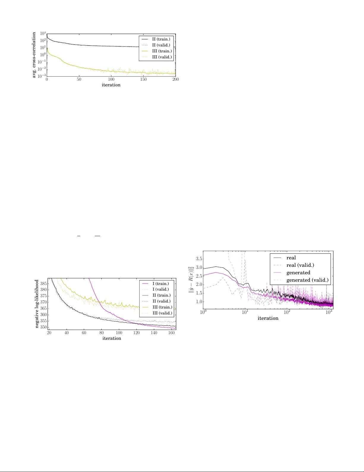
1 Enabling Dark Ener gy Science with Deep Generati v e Models of Galaxy Images Siamak Rav anbakhsh 1 , Franc ¸ ois Lanusse 2 , Rachel Mandelbaum 2 , Jef f Schneider 1 , and Barnab ´ as P ´ oczos 1 1 School of Computer Science, Carne gie Mellon University 2 McW illiams Center for Cosmology , Carne gie Mellon University Abstract —Understanding the nature of dark energy , the mys- terious for ce driving the accelerated expansion of the Universe, is a major challenge of modern cosmology . The next generation of cosmological surveys, specifically designed to address this issue, rely on accurate measurements of the apparent shapes of distant galaxies. Howev er , shape measurement methods suffer fr om various unavoidable biases and theref ore will rely on a precise calibration to meet the accuracy requir ements of the science analysis. This calibration process remains an open challenge as it requir es large sets of high quality galaxy images. T o this end, we study the application of deep conditional generative models in generating realistic galaxy images. In particular we consider variations on conditional variational autoencoder and introduce a new adversarial objective f or training of conditional generative networks. Our results suggest a reliable alternative to the acquisition of expensive high quality observations for generating the calibration data needed by the next generation of cosmological surveys. The last two decades hav e greatly clarified the contents of the Uni verse, while leaving se veral lar ge mysteries in our cos- mological model. W e now have compelling evidence that the expansion rate of the Univ erse is accelerating, suggesting that the vast majority of the total energy content of the Univ erse is the so-called dark ener gy . Y et we lack an understanding of what dark energy actually is, which provides one of the main motiv ations behind the next generation of cosmological surve ys such as LSST LSST Science Collaboration et al. ( 2009 ), Euclid Laureijs et al. ( 2011 ) and WFIRST Green et al. ( 2012 ). These billion dollar projects are specifically designed to shed light on the nature of dark energy by probing the Univ erse through the weak gravitational lensing effect – i.e . , the minute deflection of the light from distant objects by the intervening massi ve large scale structures of the Univ erse. On cosmological scales, this lensing ef fect causes very small but coherent deformations of background galaxy images, which appear slightly shear ed , pro viding a w ay to statistically map the matter distribution in the Universe. T o measure the lensing signal, future surveys will image and measure the shapes of billions of galaxies, significantly dri ving down statistical errors compared to the current generation of surve ys, to the lev el where dark energy models may become distinguishable. Howe ver , the quality of this analysis hinges on the accuracy of the shape measurement algorithms tasked with estimating the ellipticities of the galaxies in the survey . This point is particularly crucial to the success of these missions, as any unaccounted for measurement biases in their ensemble av erages would impact the final cosmological analysis and potentially lead to false conclusions. In order to detect and/or calibrate any such biases, future surveys will heavily rely on image simulations, closely mimicking real observations but with a known ground truth lensing signal. Galaxies Propagation through the Universe Stars Propagation through the Earth’s atmosphere and telescope optics Realisation on detector (sheared) (pixellated) (blurred) (pixellated) (blurred) Fig. 1: Illustration of the processes in volved in the measurement of weak gra vitational lensing. The light from distant galaxies is deflected by the matter in the Universe, causing a shearing of the galaxy images, which are then further blurred by the atmosphere and the telescope optics and finally pixelated into a noisy image by the imaging sensor . Image credit: Mandelbaum et al. ( 2014 ), adapted from Kitching et al. ( 2010 ). Producing these image simulations, ho wever , is challenging in itself as the y require high quality galaxy images as the input of the simulation pipeline. Such observations can only be obtained by e xtremely expensi ve space-based imaging surve ys, which will remain a scarce resource for the foreseeable future. The largest current surve y being used for image simulation purposes is the C O S M O S surve y Scoville et al. ( 2007 ), carried out using the Hubble Space T elescope (HST). Despite being the largest available dataset, C O S M O S is relatively small, and there is great interest in increasing the size of our galaxy image samples to impro ve the quality of this crucial calibration process. In this work, we propose an alternativ e to the expensiv e acquisition of more high quality calibration data using deep conditional generative models. In recent years, these models hav e achie ved remarkable success in modeling complex high- dimensional distributions, producing natural images that can pass the visual T uring test. T wo prominent approaches for training these models are variational autoencoder (V AE) Kingma and W elling ( 2013 ); Rezende et al. ( 2014 ) and generative adversarial network (GAN) Goodfellow et al. ( 2014 ). Our aim is to train a coditional variation of these models using existing HST data and generate new galaxy 2 Fig. 2: Samples from the G A L A X Y - Z O O dataset versus generated samples using conditional generativ e adversarial network of Section III . Each synthetic image is a 128 × 128 colored image (here inv erted) produced by conditioning on a set of features y ∈ [0 , 1] 37 . The pair of observed and generated images in each column correspond to the same y value. For details on these crowd-sourced y features see W illett et al. ( 2013 ). These instances are selected from the test-set and were unav ailable to the model during the training. images “conditioned” on statistics of interest such as the brightness or size of the galaxy . This will allo w us to syn- thesize calibration datasets for specific galaxy populations, with objects exhibiting realistic morphologies. In related works in machine learning literature Regier et al. ( 2015b ) use a con ve x combination of smooth and spiral templates in an (unconditioned) generativ e model of galaxy images and Regier et al. ( 2015a ) propose using V AE for this task. 1 In the following, Section I giv es a brief background on the image generation for calibration and its significance for mod- ern cosmology . W e then re view the current approaches to deep conditional generativ e models and introduce ne w techniques for our problem setting in Sections II and III . In Section IV we assess the quality of the generated images by comparing the conditional distributions of shape and morphology parameters between simulated and real galaxies, and find good agreement. I . W E A K G R A V I TA T I O N A L L E N S I N G In the weak re gime of gra vitational lensing, the distortion of background galaxy images can be modeled by an anisotropic shear , noted γ , whose amplitude and orientation depend on the matter distribution between the observer and these distant galaxies. This shear affects in particular the apparent ellipticity of galaxies, denoted e . Measuring this weak lensing effect is made possible under the assumption that background galaxies are randomly oriented, so that the ensemble a verage of the shapes would average to zero in the absence of lensing. Their apparent ellipticity e can then be used as a noisy but unbiased estimator of the shear field γ : E [ e ] = γ . The cosmological 1 The current approach to address this problem in cosmology literature is to fit analytic parametric light profiles (defined by size, intensity , ellipticity and steepness parameters) to the observed galaxies, followed by a simple modelling of the distribution of the fitted parameters as a function of a quantity of interest, such as the galaxy brightness. This modelling usually simply in volves fitting a linear dependence of mean and standard deviation of a Gaussian distribution – e.g. , see Hoekstra et al. ( 2016 ); Appendix A. Howe ver , simple parametric models of galaxy light profiles do not have the complex morphologies needed for calibration task. The only currently av ailable alternati ve, if realistic galaxy morphologies are needed, is to use the training set images themselves as the input of the simulation pipeline. This in volves subsampling the training set to match the distribution of size, redshift and brightness of the target galaxy simulations, lea ving only a relati vely small number of objects, reused several hundred times to simulate a large surve y – e.g. , see Jarvis et al. ( 2016 ); Section 6.1. analysis then in volv es computing auto- and cross-correlations of the measured ellipticities for galaxies at different distances. These correlation functions are compared to theoretical pre- dictions in order to constrain cosmological models and shed light on the nature of dark energy . Howe ver , measuring galaxy ellipticities such that their ensemble av erage (used for the cosmological analysis) is unbiased is an extremely challenging task. Fig. 1 illustrates the main steps in volved in the acquisition of the science images. The weakly sheared galaxy images under go additional distortions (essentially blurring) as they go through the at- mosphere and telescope optics, before being acquired by the imaging sensor which pixelates the noisy image. As this figure illustrates, the cosmological shear is clearly a subdominant effect in the final image and needs to be disentangled from subsequent blurring by the atmosphere and telescope options. This blurring, or Point Spread Function (PSF), can be directly measured by using stars as point sources, as shown at the top of Fig. 1 . Once the image is acquired, shape measurement algorithms are used to estimate the ellipticity of the galaxy while correct- ing for the PSF . Howe ver , despite the best efforts of the weak lensing community for nearly two decades, all current state- of-the-art shape measurement algorithms are still susceptible to biases in the inferred shears. These measurement biases are commonly modeled in terms of additi ve and multiplicativ e bias parameters c and m defined as: E [ e ] = (1 + m ) γ + c (1) where γ is the true shear . Depending on the shape measure- ment method being used, m and c can depend on factors such as the PSF size/shape, the lev el of noise in the images or , more generally , intrinsic properties of the galaxy population (like their size and ellipticity distrib utions, etc. ). Calibration of these biases can be achieved using image simulations, closely mimicking real observations for a given survey but using galaxy images distorted with a kno wn shear , thus allo wing the measurement of the bias parameters in Eq. ( 1 ). Image simulation pipelines , such as the GalSim package Rowe et al. ( 2015 ), use a forward modeling of the observa- tions, reproducing all the steps of the image acquisition pro- 3 Fig. 3: Samples from the C O S M O S dataset and generated samples using the conditional variational autoencoder (C-V AE, scheme I) and our variation on conditional generati ve adv ersarial network (C-GAN). Each column image sho ws three 64 × 64 images (here inv erted) produced by conditioning on the same set of features y ∈ < 3 in the test-set. Due to its high dynamic range, most figures are v ery faint. In the bottom three rows, each image is individually normalized. cess in Fig. 1 , and therefore require as a starting point galaxy images with high resolution and S/N. The main difficulty in these image simulations is therefore the need for a calibration sample of high quality galaxy images representati ve of the galaxy population of the survey being simulated. Our aim in this work is to train a deep generati ve model which can be used to cheaply synthesize such data sets for specific galaxy populations, by conditioning the samples on measurable quan- tities. A. Data set As our main dataset, we use the C O S M O S survey to build a training and validation set of galaxy images and extract from the corresponding catalog a condition vector y with three features: half-light radius (measure of size), magnitude (measure of brightness) and redshift (cosmological measure of distance). T o facilitate the training, we align all galaxies along their major axis and produce 85,000 instances of 64x64 image stamps using the GalSim package. W e also use the G A L A X Y - Z O O dataset W illett et al. ( 2013 ) to demonstrate the abilities of our alternative conditional adversarial objective. Each of the 61,000 galaxy images in this dataset is accompanied by y ∈ [0 , 1] 37 features produced using a crowd-sourced set of questions that form a decision tree. W e cropped the central 50% of these images and resized them to 128 × 128 pix els. W e augmented both datasets by flipping the images along the vertical and horizontal axes. I I . C O N D I T I O N A L V A R I A T I O N A L A U T O E N C O D E R Applications in semi-supervised learning and structured pre- diction have motiv ated different versions of the “conditional” variational autoencoder (C-V AE) in the past Kingma et al. ( 2014 ); Sohn et al. ( 2015 ). Although the architecture that we discuss here resembles to those of Kingma et al. ( 2014 ); Sohn et al. ( 2015 ), there are some differences due to different objectiv es. W e are interested in learning the conditional density p ∗ ( x | y ) for x ∈ X and y ∈ Y , gi ven a set of observ ations D = ( ˆ x 1 , ˆ y 1 ) , . . . , ( ˆ x N , ˆ y N ) , by learning model parameters θ that maximizes the conditional likelihood Q ( ˆ x, ˆ y ) ∈D p θ ( ˆ x | ˆ y ) – e .g. , for the C O S M O S dataset X = < 64 × 64 and Y = < 3 . In a latent-variable model , an auxiliary variable z ∈ Z is introduced to increase the expressi ve power of p θ ( x, z | y ) , such that R Z p θ ( x, z | y )d z is the marginal of interest. Here, different assignments to z can explain variations and complex statistical dependencies in p ( x | y ) . T o enable efficient (ancestral) sampling from this model, p θ can be a directed model p θ ( x, z | y ) = p θ 1 ( z | y ) p θ 2 ( x | z , y ) , where we first sample z ∼ p θ 1 ( · | y ) follo wed by x ∼ p θ 2 ( · | z , y ) . An expressiv e form for the conditional distributions p θ 1 and p θ 2 is a deep neural network, that can represent complex directed graphical models. Here, for example, we model p θ 2 ( x | z , y ) using multi-layered con volutional or densely connected neural networks that encode the mean and variance of a multi-variate Gaussian for the C O S M O S dataset and the e xpectation of Bernoulli variables for the G A L A X Y - Z O O dataset. T o learn the parameters θ one needs to estimate the posterior p θ ( z | x, y ) , which is often intractable in directed models. An elegant solution to this problem is to introduce a second directed model q ( z | x, y ) , called inference or r ecognition model . This conditional distribution is also encoded as a deep neural network and it is tasked with estimating the intractable posterior p θ ( z | x, y ) . This is achieved through a variational bound on the conditional log-likelihood: log( p θ ( ˆ x | ˆ y )) ≥ − D KL ( q φ ( z | ˆ x, ˆ y ) k p θ 1 ( z | ˆ y )) (2) + E z ∼ q φ ( ·| ˆ x, ˆ y ) [log p θ 2 ( ˆ x | z , ˆ y )] where the first term is the KL-di vergence between the posterior q φ and the conditional prior p θ 1 and the second term is the reconstruction error – that is we want the model to achieve lo w reconstruction error while encoding the dataset. At the same time the KL-di ver gence term encourages the code to follo w a distribution, dictated by the the condition y . Fortunately , the reparametrization-trick by Kingma and W elling ( 2013 ); Rezende et al. ( 2014 ); W illiams ( 1992 ) enables the maxi- mization of this lower-bound ( i.e. , learn θ 1 , θ 2 and φ ) using stochastic back-propagation through the layers of these three neural networks. This enables maximizing the log-likelihood of an e xpressiv e model with lar ge number of parameters through variations of stochastic gradient descent. 4 0 50 100 150 200 iteration 10 − 3 10 − 2 10 − 1 10 0 10 1 10 2 10 3 a vg . cross-correlation II (train.) II (valid.) III (train.) III (valid.) Fig. 4: Cross-correlation between y and z in C-V AE when p ( z | y ) = p ( z ) , with and without cross-correlation penalty . A. Cr oss-Corr elation Inspired by the application of cross-correlation in disentan- gling the factors in an autoencoder by Cheung et al. ( 2014 ), we also consider an alternativ e method of conditioning in V AE. Let us proceed with a simple question: what happens here if we simplify the prior p θ 1 ( z | y ) ⇒ p θ 1 ( z ) ? In princi- ple, the simplified C-V AE w ould try to make the posterior q φ ( z | x, y ) independent of y . 2 In this case, for generating samples x ∼ p θ ( · | y ) , we could still sample z ∼ p θ 1 ( · ) and then generate x ∼ p θ 2 ( · | y , z ) . In practice, we observe z and y become more and more decorrelated during the training, but this happens at a slow pace. W e can further enforce this decorrelation using a mini- batch cross-correlation penalty C ( { ˆ y } , { z } ) def = 1 2 X i,j  1 N N X n =1 ( ˆ y ( n ) i − ¯ y i )( z ( n ) i − ¯ z i )  2 where { ˆ y } / { z } are conditions/codes in a mini-batc h of size N , where z ∼ q ψ ( · | ˆ x ) and i, j index dimensions of ˆ y , z respectiv ely . Here ¯ y i and ¯ z i are mini-batch average values. 20 40 60 80 100 120 140 160 iteration 350 355 360 365 370 375 380 385 negative log-likelihood I (train.) I (valid.) II (train.) II (valid.) III (train.) III (valid.) Fig. 5: Negati ve log-likelihood of different C-V AE schemes. Note that scheme II can only serve as a baseline and due to correlation between ˆ y and z cannot be used for conditional sampling. Lack of cross-correlation only entails independence, if both y i and z i hav e Gaussian distribution. Although p θ 1 ( z ) is by design a standard Gaussian, the condition y may have an arbitrary distribution. T o resolve this, we transform ˆ y i → F − 1 N ( F y i ( ˆ y i )) , where F y i is the empirical cumulativ e distri- bution function (CDF) for ˆ y ∈ D and F − 1 N is the (numerically 2 This is because the information content of y is already available to the generativ e model p θ ( x | y , z ) for reconstruction and reducing the information exchange through z should reduce the KL-div ergence penalty D KL ( q φ ( z | ˆ x, ˆ y ) k p ( z )) . approximated) inv erse CDF of Gaussian. The transformed variable has a Gaussian distribution. B. Experiments Figure 4 compares the reduction in the a verage cross- correlation between ˆ y and z for the same network, with and without the cross-correlation penalty . For numerical stability we linearly increase the penalty coef ficient from 0 to 1000 ov er iterations. These results are for the C O S M O S dataset. All C-V AE results are using the log-pixel-intensity , also for numerical stability . Figure 5 compares − log( p θ ( ˆ x | ˆ y )) for three models: I using a neural network to encode p θ 1 ( z | y ) II using p θ 1 ( z | y ) = p θ 1 ( z ) III p θ 1 ( z | y ) = p θ 1 ( z ) plus cross-correlation penalty The figure suggests that the first scheme ev entually produces better models. It also shows that enforcing the independence of z and y only slightly decreases the likelihood, compared to the baseline II where z and y remain highly dependent. I I I . A N E W O B J E C T I V E F O R A DV E R S A R I A L T R A I N I N G A major problem with V AE-generated images is their blur- riness. A few recent works address this issue Kingma et al. ( 2016 ); Larsen et al. ( 2015 ); Doso vitskiy and Brox ( 2016 ) – e.g. , by defining a more expressiv e reconstruction loss. Fortunately , the noise model is av ailable for C O S M O S images, and the added noise to some extent reduces this problem in our application (see Section IV ). 10 0 10 1 10 2 10 3 iteration 1 . 0 1 . 5 2 . 0 2 . 5 3 . 0 3 . 5 k ˆ y − R ( x ) k 2 2 real real (valid.) generated generated (valid.) Fig. 6: The prediction error for real and generated images in C-GAN for C O S M O S dataset. An alternative to generativ e modeling that does not suffer from this problem is offered by adversarial training of genera- tiv e networks Goodfellow et al. ( 2014 ). In the adversarial setting , a generator G ω : Z → X attempts to fool the discriminator D ψ : X → [0 , 1] into classifying its fak e instances x = G ( z ) as real, while the discriminator’ s objecti ve is to correctly classify the two sources of real versus gener- ated instances. Deep networks representing these adversaries are trained alternativ ely , and under some conditions p G (the implicit distribution of the generator G ω for z ∼ U (0 , 1) ) con ver ges to p ∗ – i.e. , at this fixed-point, the generator produces realistic images that are indistinguishable by the discriminator . The conditional variation of this method was first intro- duced by Mirza and Osindero ( 2014 ) and used in a cascade 5 CVAE sample CVAE sample + noise COSMOS image Fig. 7: Comparison of a C-V AE sample before and after adding noise and a real C O S M O S image with corresponding size, magnitude and redshift. of conditional models with increasing resolution in Denton et al. ( 2015 ). In these conditional models, the generator G ω : Z × Y → X and the discriminator D ψ : X × Y → [0 , 1] , are both deep neural networks that are no w conditioned on the same observed variable ˆ y ∈ D . The min-max formulation of this adversarial setting seeks a saddle-point for min ω max ψ E ˆ x, ˆ y ∈D ,z ∈U  log( D ψ ( ˆ x, ˆ y )) + log(1 − D ψ ( G ω ( z , ˆ y ) , ˆ y ))  In practice it is much more efficient to use a different loss function for the generator as it produces stronger gradients for the generator at the beginning Goodfellow et al. ( 2014 ): max ψ E ˆ x, ˆ y ∈D ,z ∈U  log( D ψ ( ˆ x, ˆ y ))+ log(1 − D ψ ( G ω ( z , ˆ y ) , ˆ y ))  max ω E z ∈U  log( D ψ ( G ω ( z , ˆ y ) , ˆ y ))  Here, one must carefully adjust the expressi ve power of G and D to av oid oscillations, and domination of either adversary . The choice of hyper-parameters is known to be a major hurdle in training of adversarial networks and using this scheme, despite much effort, we could not train a generator for our problem that uses continuous conditional variables. W e introduce an alternative adversarial objective for conditional generative modeling that in our experience is more stable and did not require any hyper-parameter tuning in our application. The basic idea is simple: A predictor R : X → Y replaces the discriminator D : X × Y → [0 , 1] . The predictor attempts to produce predictions of the condition ˆ y ∈ D for the real data, that are at least as good as its predictions for generated instances. The generator’ s objectiv e is to produce instances with low prediction error Predictor: min ψ min { 0 , (3) E ˆ x, ˆ y ∈D ,z ∈U  ` ( R ψ ( G ω ( z , ˆ y )) , ˆ y ) − ` ( R ψ ( x ) , ˆ y )  } Generator: min ω E ˆ y ∈D ,z ∈U  ` ( R ψ ( G ω ( z , ˆ y )) , ˆ y )  (4) where in our application ` ( y , ˆ y ) = k y − ˆ y k 2 2 . Why should the generator produces realistic images at all as long as the predictor makes equally bad predictions for both real and generated images? Both errors Eqs. ( 3 ) and ( 4 ) will be low in this case. The ke y here is that the generator always seeks to impro ve its samples to increase their prediction (a) Galaxy sizes (b) Galaxy brightness Fig. 8: Comparison of galaxy sizes and brightness between real C O S M O S images and C-V AE samples. Colors indicate the value of the relev ant variable used to condition the generated images (half-light radius for size and magnitude for brightness) accuracy and therefore the dynamics of this adv ersarial setting does not allow this mode of failure. This scheme, also relaxes the constraint on the expressiv e power of the adversaries . This is because the predictor has no incentive to lower the error for the real data, as long as its prediction errors are not worse that those of the generated data. Therefore, it is only the generator that fuels the competition and training is practically finished when the generator is unable to improve. A mode of failure that our scheme does not resolve is the collapse of generator , where generator G ( y, z ) repeats few output patterns by solely relying on y and basically ignoring the random feed z . The predictor e ventually realizes this repeating pattern in generated data but gradient descent can no longer rescue the generator from this local optima. A solution to this problem called mini-batch discrimination was recently proposed by Salimans et al. ( 2016 ), where each instance in the mini-batch is augmented with information about its dif ferences with other instances in the same mini-batch. The Predictor can therefore detect this tendency of the generator early on, and the generator incurs a loss for its beha vior before its complete collapse. For better mini-batch statistics, we use relativ ely larger mini-batches with 128/256 instances. A. Experiments Follo wing Radford et al. ( 2015 ) we use (de)con volutional layers with (fractional) stride, batch normalization Ioffe and Szegedy ( 2015 ) and leak y-ReLU activ ation functions in our deep networks. For optimization, we use Adam Kingma and Ba ( 2014 ) with reduced exponential decay rate of .5 for the first moment estimates. Figure 6 reports the prediction loss ` ( R ψ ( G ω ( z , ˆ y ) , ˆ y )) and ` ( R ψ ( x ) , ˆ y ) for the C O S M O S dataset, were we use 4 (de)con volution layers. The figure suggests that the predictor tends to keep the prediction error of the real images slightly higher than that of generated images. Both of these quantities reduce over time, and their agreement with validation errors could monitor con vergence. The fact that the error is decreas- ing over time and prediction error for both real and generated data remains close to each other is due to having a “laid back” predictor – i.e . , by removing the min(0 , . ) operation in predictor’ s loss, we would lose both of these properties. For illustration purposes, we applied the same method to the G A L A X Y - Z O O dataset. Figure 2 sho ws some instances 6 in the test-set accompanied by C-GAN generated image conditioned on the same ˆ y . For this dataset we used 5- layer fully (de)conv olutional generator and predictor , mini- batch discrimination, batch-normalization and tanh acti vation function for the final layer of the generator . I V . V A L I D A T I O N In this section, we assess the quality of the model generated galaxy images by comparing common image statistics used in weak lensing analyses. Our aim is to consistently measure the same statistics on real C O S M O S images and images generated by our model for the same set of input v ariables y . These statistics are affected by the presence of noise in the image, but as was noted in the previous section, our C-V AE generates essentially noiseless images, which pre vents direct comparison with real images. W e limit this analysis to C-V AE generated images (as we found it to produce more consistent results compared to C-GAN) and add a noise field to our generated images. This noise model, calibrated for C O S M O S observa- tions, is provided by the GalSim package; see Fig. 7 . The most commonly used image statistics in weak lensing analyses rely on the second moments of the galaxy’ s intensity profile I ( u 1 , u 2 ) , where ( u 1 , u 2 ) are pixel coordinates. The second moment tensor Q is defined as: Q αβ = R d u 1 d u 2 W ( u 1 , u 2 ) I ( u 1 , u 2 ) u α u β R d u 1 d u 2 W ( u 1 , u 2 ) I ( u 1 , u 2 ) , with ( α, β ) ∈ { 1 , 2 } and where W is a weighting func- tion. This tensor can be used to define a size measurement σ = | det( Q ) | 1 / 4 which reduces to the standard deviation if the light profile is a Gaussian. More importantly , the second moments are commonly used to measure galaxy ellipticities which can be defined as: e = e 1 + ie 2 = Q 11 − Q 22 − 2 iQ 12 Q 11 + Q 22 + 2( Q 11 Q 22 − Q 2 12 ) 1 / 2 T o measure Q in practice, we use the adaptive moments method Hirata and Seljak ( 2003 ); Mandelbaum et al. ( 2005 ) which estimates the second order moments by fitting an elliptical Gaussian profile to the galaxy light profile. As a side product of this method, we can also use the amplitude of the best fit Gaussian model as a proxy for the brightness of the galaxy . W e compare real C O S M O S images to C-V AE samples by processing the images in pairs, where e very C O S M O S galaxy in our validation set is associated to a C-V AE sample conditioned on the half-light radius, magnitude and redshift of the real galaxy . Fig. 8a shows for each pair of images the galaxy size σ , as measured using second order moments; see also Fig. 3 . The color of the points indicates the half-light radius of the C O S M O S galaxy in the pair , also used to condition the C-V AE sample. As can be seen, the sizes of generated galaxies are generally unbiased. Fig. 8b shows the similar results for brightness; C-V AE is generating samples of the correct brightness without any significant bias. The most relev ant image statistics for weak lensing science are the ellipticity and size distributions of a giv en galaxy sample. Fig. 9 compares these overall distributions measured 0.0 0.1 0.2 0.3 0.4 0.5 0.6 0.7 0.8 E l l i p t i c i t y | e | 0.0 0.5 1.0 1.5 2.0 2.5 3.0 COSMOS galaxies CVAE samples 0 2 4 6 8 10 12 14 16 S i z e σ [ p i x ] 0.00 0.05 0.10 0.15 0.20 COSMOS galaxies CVAE samples Fig. 9: Comparison of galaxy ellipticity (left) and size (right) distributions measured from second moments between real C O S - M O S images and CV AE samples. on real and generated galaxies. Note that contrary to the pre vi- ous test where the quantities considered (size and brightness) were part of the condition v ariable y , the ellipticity is not. Therefore, this test allows us to check how well the model is able to blindly learn correct galaxy shapes. This figure shows that despite being slightly more elliptical than real galaxies, the ellipticity distribution of the C-V AE samples is broadly consistent with the C O S M O S distribution. Fig. 9 also compares size distributions which are in good agreement. This comes as no surprise howe ver as C-V AE samples are explicitly conditioned on galaxy sizes and the previous test has shown these samples to be largely unbiased. C O N C L U S I O N In this paper, we proposed novel techniques and studied the application of two most promising methods for deep conditional generative modeling in producing galaxy images. In the future, we plan to measure more subtle morphological statistics in generated images and find ways for simultaneous learning of the noise model. W e are also in vestigating the application of our variation on adversarial training in other settings and assessing the effecti veness of the predictor as a stand-alone classification/regression model. R E F E R E N C E S Brian Cheung, Jesse A Liveze y , Arjun K Bansal, and Bruno A Olshausen. Discov ering hidden factors of variation in deep networks. arXiv preprint , 2014. Emily L Denton, Soumith Chintala, Rob Fergus, et al. Deep generativ e image models using a laplacian pyramid of adversarial networks. In Advances in Neur al Information Pr ocessing Systems , pages 1486–1494, 2015. Alex ey Doso vitskiy and Thomas Brox. Generating images with perceptual similarity metrics based on deep networks. arXiv preprint arXiv:1602.02644 , 2016. Ian Goodfello w , Jean Pouget-Abadie, Mehdi Mirza, Bing Xu, David W arde-F arley , Sherjil Ozair , Aaron Courville, and Y oshua Bengio. Generativ e adv ersarial nets. In Advances in Neural Information Pr ocessing Systems , pages 2672–2680, 2014. 7 J. Green, P . Schechter, C. Baltay , R. Bean, D. Bennett, R. Brown, C. Conselice, M. Donahue, et al. W ide-Field InfraRed Survey T elescope (WFIRST) Final Report. ArXiv e-prints , August 2012. C. Hirata and U. Seljak. Shear calibration biases in weak- lensing surveys. Monthly Notices of the Royal Astr onom- ical Society , 343:459–480, August 2003. doi: 10.1046/j. 1365- 8711.2003.06683.x. Henk Hoekstra, Massimo V iola, and Ricardo Herbonnet. A study of the sensitivity of shape measurements to the input parameters of weak lensing image simulations. arXiv pr eprint arXiv:1609.03281 , 2016. Serge y Ioffe and Christian Szegedy . Batch normalization: Accelerating deep network training by reducing internal cov ariate shift. arXiv pr eprint arXiv:1502.03167 , 2015. M Jarvis, E Sheldon, J Zuntz, T Kacprzak, SL Bridle, A Amara, R Armstrong, MR Becker , GM Bernstein, C Bon- nett, et al. The des science verification weak lensing shear catalogues. Monthly Notices of the Royal Astr onomical Society , 460(2):2245–2281, 2016. Diederik Kingma and Jimmy Ba. Adam: A method for stochastic optimization. arXiv pr eprint arXiv:1412.6980 , 2014. Diederik P Kingma and Max W elling. Auto-encoding varia- tional bayes. arXiv pr eprint arXiv:1312.6114 , 2013. Diederik P Kingma, Shakir Mohamed, Danilo Jimenez Rezende, and Max W elling. Semi-supervised learning with deep generati ve models. In Advances in Neural Information Pr ocessing Systems , pages 3581–3589, 2014. Diederik P . Kingma, T im Salimans, and Max W elling. Improv- ing v ariational inference with in verse autoregressi ve flow . arXiv:1606.04934 , 2016. T . Kitching, S. Balan, G. Bernstein, M. Bethge, S. Bridle, F . Courbin, M. Gentile, A. Hea vens, et al. Gra vitational Lensing Accuracy T esting 2010 (GREA T10) Challenge Handbook. ArXiv e-prints , September 2010. Anders Boesen Lindbo Larsen, Søren Kaae Sønderby , and Ole Winther . Autoencoding beyond pixels using a learned similarity metric. arXiv pr eprint arXiv:1512.09300 , 2015. R. Laureijs, J. Amiaux, S. Arduini, J. . Augu ` eres, J. Brinch- mann, R. Cole, M. Cropper , C. Dabin, L. Duvet, A. Ealet, and et al. Euclid Definition Study Report. ArXiv e-prints , October 2011. LSST Science Collaboration, P . A. Abell, J. Allison, S. F . Anderson, J. R. Andre w , J. R. P . Angel, L. Armus, D. Arnett, S. J. Asztalos, T . S. Axelrod, and et al. LSST Science Book, V ersion 2.0. ArXiv e-prints , December 2009. R. Mandelbaum, C. M. Hirata, U. Seljak, J. Guzik, N. Pad- manabhan, C. Blake, M. R. Blanton, R. Lupton, and J. Brinkmann. Systematic errors in weak lensing: applica- tion to SDSS galaxy-galaxy weak lensing. Monthly Notices of the Royal Astr onomical Society , 361:1287–1322, August 2005. doi: 10.1111/j.1365- 2966.2005.09282.x. R. Mandelbaum, B. Rowe, J. Bosch, C. Chang, F . Courbin, M. Gill, M. Jarvis, A. Kannawadi, et al. The Third Grav- itational Lensing Accuracy T esting (GREA T3) Challenge Handbook. The Astrophysical Journal Supplement , 212:5, May 2014. doi: 10.1088/0067- 0049/212/1/5. Mehdi Mirza and Simon Osindero. Conditional generati ve adversarial nets. arXiv preprint , 2014. Alec Radford, Luke Metz, and Soumith Chintala. Un- supervised representation learning with deep con volu- tional generative adversarial networks. arXiv pr eprint arXiv:1511.06434 , 2015. J Regier , J McAuliffe, and Prabhat. A deep generativ e model for astronomical images of galaxies. NIPS W orkshop: Advances in Approximate Bayesian Inference, 2015a. Jeffre y Regier , Andrew Miller , Jon McAuliffe, Ryan Adams, Matt Hoffman, Dustin Lang, David Schlegel, and Mr Prab- hat. Celeste: V ariational inference for a generati ve model of astronomical images. In Proceedings of the 32nd Inter- national Conference on Machine Learning , 2015b. Danilo Jimenez Rezende, Shakir Mohamed, and Daan Wier - stra. Stochastic backpropagation and approximate inference in deep generativ e models. arXiv pr eprint arXiv:1401.4082 , 2014. B. T . P . Rowe, M. Jarvis, R. Mandelbaum, G. M. Bernstein, J. Bosch, M. Simet, J. E. Meyers, T . Kacprzak, et al. GALSIM: The modular galaxy image simulation toolkit. Astr onomy and Computing , 10:121–150, April 2015. doi: 10.1016/j.ascom.2015.02.002. T im Salimans, Ian Goodfellow , W ojciech Zaremba, V icki Cheung, Alec Radford, and Xi Chen. Improv ed techniques for training gans. arXiv preprint , 2016. N. Scoville, H. Aussel, M. Brusa, P . Capak, C. M. Carollo, M. Elvis, M. Giavalisco, L. Guzzo, et al. The Cosmic Evolution Surv ey (COSMOS): Overvie w. The Astr ophysical Journal Supplement Series , 172:1–8, September 2007. doi: 10.1086/516585. Kihyuk Sohn, Honglak Lee, and Xinchen Y an. Learning struc- tured output representation using deep conditional genera- tiv e models. In Advances in Neural Information Pr ocessing Systems , pages 3483–3491, 2015. Kyle W W illett, Chris J Lintott, Steven P Bamford, Karen L Masters, Brooke D Simmons, Ke vin R V Casteels, Ed- ward M Edmondson, Lucy F Fortson, et al. Galaxy zoo 2: detailed morphological classifications for 304 122 galaxies from the sloan digital sky survey . Monthly Notices of the Royal Astronomical Society , page stt1458, 2013. Ronald J W illiams. Simple statistical gradient-follo wing al- gorithms for connectionist reinforcement learning. Machine learning , 8(3-4):229–256, 1992. 8 A P P E N D I X C - G A N R E S U LT S This appendix complements Section IV by providing the results of the C-GAN on the C O S M O S data. Follo wing the same approach as for the v alidation of the C-V AE results, we first compare size and brightness statistics measured on pairs of real C O S M O S images and C-GAN samples, with same conditional v alues. As can be seen in Fig. 10 , the size and brightness of the g alaxies generated by the C-GAN are largely unbiased and similar to the C-V AE results. (a) Galaxy sizes (b) Galaxy brightness Fig. 10: Comparison of galaxy sizes and brightness between real C O S M O S images and C-GAN samples. Colors indicate the value of the relev ant variable used to condition the generated images (half- light radius for size and magnitude for brightness) 0.0 0.1 0.2 0.3 0.4 0.5 0.6 0.7 0.8 E l l i p t i c i t y | e | 0.0 0.5 1.0 1.5 2.0 2.5 3.0 COSMOS galaxies C-GAN samples 0 2 4 6 8 10 12 14 16 S i z e σ [ p i x ] 0.00 0.05 0.10 0.15 0.20 COSMOS galaxies C-GAN samples Fig. 11: Comparison of galaxy ellipticity (left) and size (right) distributions measured from second moments between real C O S - M O S images and C-GAN samples.