BayesVarSel: Bayesian Testing, Variable Selection and model averaging in Linear Models using R

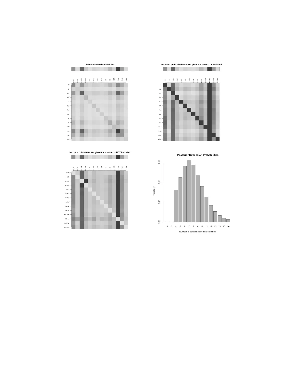
Ba y esV arSel: Ba y esian T esting, V ariable Selection and mo del a v eraging in Linear Mo dels using R Gonzalo Garcia-Donato 1 and Anab el F orte 2 1 Univ ersidad de Castilla La Manc ha; 2 Univ ersidad de V alencia Ma y 2, 2018 Abstract This pap er introduces the R pack age Bay esV arSel whic h imple- men ts ob jectiv e Ba y esian metho dology for h yp othesis testing and v ari- able selection in linear mo dels. The pac k age computes p osterior prob- abilities of the comp eting h yp otheses/models and provides a suite of to ols, sp ecifically proposed in the literature, to properly summarize the results. Additionally , Bay esV arSel is armed with functions to compute several t yp es of mo del av eraging estimations and predictions with weigh ts given by the p osterior probabilities. Ba yesV arSel con- tains exact algorithms to p erform fast computations in problems of small to mo derate size and heuristic sampling methods to solve large problems. The soft ware is in tended to app eal to a broad sp ectrum of users, so the in terface has b een carefully designed to b e highly intuiti- tiv e and is inspired by the well-kno wn lm function. The issue of prior inputs is carefully addressed. In the default usage (fully automatic for the user) Bay esV arSel implemen ts the criteria-based priors prop osed b y Bay arri et al. (2012), but the adv anced user has the p ossibility of using sev eral other p opular priors in the literature. The pac k age is a v ailable through the Comprehensive R Arc hive Netw ork, CRAN. W e illustrate the use of Bay esV arSel with sev eral data examples. 1 1 An illustrated o v erview of Ba y esV arSel T esting and v ariable selection problems are taugh t in almost any introductory statistical course. In this first section we assume such background to present the essence of the Ba yesian approach and the basic usage of Bay esV arSel with hardly any mathematical formulas. Our motiv ating idea in this first section is mainly to present the app eal of the Bay esian answ ers to a v ery broad sp ectrum of applied researc hers. The remaining sections are organized as follo ws. In Section 2 the problem is presen ted and the notation needed is introduced join tly with the basics of the Ba yesian metho dology . Section 3 and Section 4 explain the details concerning the obtention of p osterior probabilities in h yp othesis testing and v ariable selection problems, resp ectiv ely , in Ba yesV arSel . In Section 5 sev- eral to ols to describ e the p osterior distribution are explained and Section 6 is devoted to mo del av eraging techniques. Finally , Section 7 concludes with directions that w e plan to follo w for the future of the Bay esV arSel pro ject. In the Appendix, form ulas for the most delicate ingredien t in the underly- ing problem in Bay esV arSel , namely the prior distributions for parameters within eac h mo del, are collected. 1.1 T esting In testing problems, several comp eting hypotheses, H i , ab out a phenomenon of in terest are p ostulated. The role of statistics is to pro vide summaries ab out the evidence in fav or (or against) the h yp otheses once the data, y , ha ve b een observed. There are many imp ortant statistical problems with ro ots in testing lik e mo del selection (or mo del choice) and mo del av eraging. The formal Bay esian resp onse to testing problems is based on the p oste- rior probabilities of the h yp otheses that summarize, in a fully understandable w ay , all the av ailable information. In Ba yesV arSel an ob jective p oin t of view (in the sense explained in Berger, 2006) is adopted and the rep orted p oste- rior probabilities only depend on y and the statistical mo del assumed. These ha ve hence the great app eal of b eing fully automatic for users. F or illustrativ e purp oses consider the n utrition problem in Lee (1997), p143. There it is tested, based on the following sample of 19 weigh t gains (expressed in grams) of rats, R> weight.gains<- c(134, 146, 104, 119, 124, 161, 107, 83, 113, 129, 97, 123, + 70, 118, 101, 85, 107, 132, 94) 2 whether there is a difference betw een the population means of the group with a high proteinic diet (the first 12) or the control group (the rest): R> diet<- as.factor(c(rep(1,12),rep(0,7))) R> rats<- data.frame(weight.gains=weight.gains, diet=diet) This problem (usually known as the t w o-samples t -test) is normally written as H 0 : µ 1 = µ 2 v ersus H 1 : µ 1 6 = µ 2 , where it is assumed that the w eight gains are normal with an unkno wn (but common) standard deviation. The form ulas that define each of the mo dels under the p ostulated hypotheses are in R language R> M0<- as.formula("weight.gains~1") R> M1<- as.formula("weight.gains~diet") The function to p erform Bay esian tests in Ba y esV arSel is Btest which has an intuitiv e and simple syntax (see Section 3 for a detailed description). In this example R> Btest(models=c(H0=M0, H1=M1), data=rats) Bayes factors (expressed in relation to H0) H0.to.H0 H1.to.H0 1.0000000 0.8040127 --------- Posterior probabilities: H0 H1 0.554 0.446 W e can conclude that b oth h yp otheses are similarly supp orted by the data (p osterior probabilities close to 0.5) so there is no evidence that the diet has an y impact on the av erage w eight. Another illustrative example concerns the classic dataset savings (Bels- ley , Kuh, and W elsc h, 1980) considered b y F ara w a y (2002), page 29 and dis- tributed under the pack age fara w a y . This dataset contains macro economic data on 50 different countries during 1960-1970 and the question p osed is to elucidate if dpi (p er-capita disp osable income in U.S), ddpi (p ercen t rate of c hange in p er capita disp osable income), p opulation under (o ver) 15 (75) pop15 ( pop75 ) are all explanatory v ariables for sr , the aggregate p ersonal sa ving divided b y disp osable income whic h is assumed to follo w a normal distribution. This can b e written as a testing problem ab out the regression co efficien ts asso ciated with the v ariables with hypotheses H 0 : β dpi = β ddpi = β pop 15 = β pop 75 = 0 3 v ersus the alternative, sa y H 1 , that all predictors are needed. The comp eting mo dels can b e defined as R> fullmodel<- as.formula("sr~pop15+pop75+dpi+ddpi") R> nullmodel<- as.formula("sr~1") and the testing problem can b e solv ed with R> Btest(models=c(H0=nullmodel, H1=fullmodel), data=savings) --------- Bayes factors (expressed in relation to H0) H0.to.H0 H1.to.H0 1.0000 20.9413 --------- Posterior probabilities: H0 H1 0.046 0.954 The conclusion is that there is substan tial evidence fa voring H 1 , the hypoth- esis that all considered predictors explain the resp onse sr . Of course, more hypotheses can b e tested at the same time. F or instance, a simplified v ersion of H 1 that do es not include p op15 is H 2 : β dpi = β ddpi = β pop 75 = 0 that can b e included in the analysis as R> reducedmodel<- as.formula("sr~pop75+dpi+ddpi") R> Btest(models=c(H0=nullmodel, H1=fullmodel, H2=reducedmodel), data=savings) Bayes factors (expressed in relation to H0) H0.to.H0 H1.to.H0 H2.to.H0 1.0000000 20.9412996 0.6954594 --------- Posterior probabilities: H0 H1 H2 0.044 0.925 0.031 The result clearly evidences H 1 as the b est explanation for the experiment among those considered. This scenario can be extended to c hec k whic h subset of the four co v ariates is the most suitable one to explain sr . In general, the problem of selecting the b est subset of cov ariates from a group of p oten tial ones is b etter known as v ariable selection. 4 1.2 V ariable selection V ariable selection is a multiple testing problem where eac h hypothesis pro- p oses a p ossible subset of p potential explanatory v ariables initially consid- ered. Notice that there are 2 p h yp otheses, including the simplest one stating that none of the v ariables should b e used. A v ariable selection approach to the economic example ab ov e with p = 4 has 16 hypotheses and can b e solv ed using the Btest function. Nev erthe- less, Ba yesV arSel has sp ecific facilities to handle the sp ecificities of v ariable selection problems. A main function for v ariable selection is Bvs , fully de- scrib ed in Section 4. It has a simple syntax inspired b y the well-kno wn lm function. The v ariable selection problem in this economic example can b e solv ed executing R> Bvs(formula="sr~pop15+pop75+dpi+ddpi", data=savings) The 10 most probable models and their probabilities are: pop15 pop75 dpi ddpi prob 1 * * * * 0.297315642 2 * * * 0.243433493 3 * * 0.133832367 4 * 0.090960327 5 * * * 0.077913429 6 * * 0.057674755 7 * * 0.032516780 8 * * * 0.031337639 9 0.013854369 10 * * 0.006219812 With a first lo ok at these results, we can see that the most probable mo del is the mo del with all co v ariates (probability 0.30), whic h is closely follow ed b y the one without dpi with a p osterior probabilit y of 0.24. As we will see later, a v ariable selection exercise generates a lot of v aluable information of whic h the ab ov e prin ted information is only a v ery reduced summary . This can b e accessed with sp ecific metho ds that explore the char- acteristics of ob jects of the t yp e created b y Bvs . 2 Basic form ulae The problems considered in Bay esV arSel concern Gaussian linear models. Consider a response v ariable y , size n , assumed to follo w the linear mo del 5 (the subindex F refers to full mo del) M F : y = X 0 α + X β + ε , ε ∼ N n ( 0 , σ 2 I n ) , (1) where the matrices X 0 : n × p 0 , X : n × p and the regression vector co efficien ts are of conformable dimensions. Supp ose you wan t to test H 0 : β = 0 v ersus H F : β 6 = 0 , that is, to decide whether the regressors in X actually explain the resp onse. This problem is equiv alen t to the mo del c hoice (or mo del selection) problem with competing mo dels M F and M 0 : y = X 0 α + ε , ε ∼ N n ( 0 , σ 2 I n ) , (2) and w e will refer to mo dels or hypotheses indistinctly . P osterior probabilities are based on the Bay es factors (see (Kass and Raftery, 1995)), a measure of evidence provided by Bay esV arSel when solv- ing testing problems. The Ba y es factor of H F to H 0 is B F 0 = m F ( y ) m 0 ( y ) where m F is the in tegrated likelihoo d or prior predictive marginal: m 0 ( y ) = Z M 0 ( y | α , σ ) π 0 ( α , σ ) d α dσ, and m F ( y ) = Z M F ( y | α , β , σ ) π F ( α , β , σ ) d β d α dσ. Ab o v e, π 0 and π F are the prior distributions for the parameters within eac h mo del. F rom an ob jectiv e p oin t of view (the one adopted here), these distri- butions should b e fully automatic. The assignmen t of such priors (which w e call mo del selection priors) is quite a delicate issue (see Berger and P ericchi, 2001) and has inspired man y imp ortan t con tributions in the literature. The pac k age Ba yesV arSel allo ws using man y of the most imp ortant prop osals, whic h are fully detailed in the App endix. The prior implemen ted by default is the robust prior b y Ba yarri et al. (2012) as it can be considered optimal in man y senses and is based on a foundational basis. P osterior probabilities can b e obtained as P r ( H F | y ) = B F 0 P r ( H F ) ( P r ( H 0 ) + B F 0 P r ( H F )) , P r ( H 0 | y ) = 1 − P r ( H F | y ) , 6 where P r ( H F ) is the probabilit y , a priori, that hypothesis H F is true. Similar formulas can b e obtained when more than t w o hypotheses, sa y H 1 , . . . , H N , are tested. In this case P r ( H i | y ) = B i 0 ( y ) P r ( H i ) P N j =1 B j 0 ( y ) P r ( H j ) , i = 1 , . . . , N (3) whic h is the p osterior distribution ov er the mo del space (which is the set that contains all comp eting mo dels). F or simplicitly , the formula in (3) has b een expressed, without an y loss of generalit y , using Ba yes factors to the n ull mo del but the same results would b e obtained b y fixing an y other mo del. The default definition for P r ( H i ) in testing problems is to use a constan t prior, whic h assigns the same probability to all mo dels, that is, P r ( H i ) = 1 / N . F or instance, within the mo del M 3 : y = α 1 n + β 1 x 1 + β 2 x 2 + ε w e cannot test the hypotheses H 1 : β 1 = 0 , β 2 6 = 0, H 2 : β 1 6 = 0 , β 2 = 0, H 3 : β 1 6 = 0 , β 2 6 = 0 since neither M 1 (the mo del defined by H 1 ) nor M 2 are nested in the rest. Nev ertheless, it is perfectly p ossible to test the problem with the four hypotheses H 1 , H 2 , H 3 (as just defined) plus H 0 : β 1 = 0 , β 2 = 0, but of course H 0 must b e, a priori, a plausible h yp othesis. In this last case H 0 w ould take the role of null mo del. Hyp otheses do not ha ve to b e necessarily of the type β = 0 and, if testable (see Ravishank er and Dey (2002) for a prop er definition) any linear com bination of the type C t β = 0 can b e considered a hypothesis. F or instance one can b e in terested in testing β 1 + β 2 = 0. In Bay arri and Garc ´ ıa- Donato (2007) it w as formally shown that these hypotheses can b e, through reparameterizations, reduced to hypotheses like β = 0 . In Section 3 we sho w examples of ho w to solve these testing problems in Ba yesV arSel . V ariable selection is a multiple testing problem but is traditionally pre- sen ted with conv enient specific notation that uses a p dimensional binary v ector γ = ( γ 1 , . . . , γ p ) to iden tify the models. Consider the full mo del in (1), and supp ose that X 0 con tains fix cov ariates that are b elieved to b e sure in the true mo del (b y default X 0 = 1 n that w ould mak e the intercept presen t in all the models). Then each γ ∈ { 0 , 1 } p defines a hypothesis H γ stating whic h β ’s (those with γ i = 0) corresp onding to each of the columns in X are zero. Then, the mo del asso ciated with H γ is M γ : y = X 0 α + X γ β γ + ε , ε ∼ N n ( 0 , σ 2 I n ) , (4) 7 where X γ is the matrix with the columns in X corresp onding to the ones in γ . Notice that X γ is a n × p γ matrix where p γ is the n umber of 1’s in γ . Clearly , in this v ariable selection problem there are 2 p h yp otheses or mo d- els and the n ull mo del is 2 corresp onding to γ = 0 . A particularit y of v ariable selection is that it is affected b y multiplicit y issues. This is b ecause, and sp ecially for mo derate to large p , the p ossibility of a mo del showing spurious evidence is high (just b ecause man y hypotheses are considered simultaneously). As concluded in Scott and Berger (2006) m ultiplicity must b e controlled with the prior probabilities P r ( H γ ) and the constan t prior does not control for multiplicit y . Instead, these authors pro- p ose using P r ( H γ ) =  ( p + 1)  p p γ   − 1 . (5) The assignmen t ab o v e states that mo dels of the same dimension (the di- mension of M γ is p γ + p 0 ) should hav e the same probability which must b e in versely prop ortional to the n um b er of mo dels of that dimension. In the sequel w e refer to this prior as the ScottBerger prior. Both the ScottBerger prior and the Constan t prior for P r ( H γ ) are par- ticular cases of the very flexible prior P r ( M γ | θ ) = θ p γ (1 − θ ) p − p γ , (6) where the hyperparameter θ ∈ (0 , 1) has the in terpretation of the common probabilit y that a given v ariable is included (indep enden tly of all others). The Constant prior corresp onds to θ = 1 / 2 while the ScottBerger to θ ∼ Unif(0 , 1). Ley and Steel (2009) study priors for θ of the t yp e θ ∼ B eta ( θ | 1 , b ) . (7) They argue that, on man y o ccasions the user has, a priori, some information regarding the n umber of cov ariates (among the p initially considered) that are exp ected to explain the resp onse, sa y w ? . As they explain, this information can b e translated into the analysis assigning in (7) b = ( p − w ? ) /w ? . The resulting prior sp ecification has the property that the exp ected n umber of co v ariates is precisely w ? . Straigh tforward algebra shows that assuming (7) into (6) is equiv alent to (in tegrating out θ ) P r ( M γ | b ) ∝ Γ( p γ + 1)Γ( p − p γ + b ) . (8) 8 3 Hyp othesis testing with Ba y esV arSel T ests are solv ed in Bay esV arSel with Btest whic h, in its default usage, only dep ends on t wo argumen ts: models a named list of formula -t yp e ob jects defining the mo dels compared and data the data.frame with the data. The prior probabilities assigned to hypotheses is constan t, that is, P r ( H i ) = 1 / N . This default b eha vior can b e mo dified sp ecifying prior.models = "User" join tly with the argumen t priorprobs that m ust contain a named list (with names as sp ecified in main argument models ) with the prior prob- abilities to b e used for eac h hypotheses. In the last example of Section 1.1, w e can state that the simpler mo del is t wice as likely as the other t w o as: R> Btest(models=c(H0=nullmodel, H1=fullmodel, H2=reducedmodel), data=savings, prior.models="User", priorprobs=c(H0=1/2, H1=1/4, H2=1/4)) --------- Bayes factors (expressed in relation to H0) H0.to.H0 H1.to.H0 H2.to.H0 1.0000000 21.4600656 0.7017864 --------- Posterior probabilities: H0 H1 H2 0.083 0.888 0.029 Notice that the Ba y es factor remains the same, and the c hange is in posterior probabilities. Btest tries to iden tify the simplest mo del (nested in all the others) using the names of the v ariables. If suc h mo del do es not exist, the execution of the function stops with an error message. Nevertheless, there are imp ortant situations where the simplest h yp othesis is defined through linear restrictions (sometimes known as ‘testing a subspace‘) making it very difficult to deter- mine its existence just using the names. W e illustrate this situation with an example. Consider for instance the extension of the savings example in F ara w ay (2002), page 32 where H eq p : β pop 15 = β pop 75 is tested against the full alter- nativ e. This n ull hypothesis states that the effect on personal savings, sr , of b oth segmen ts of p opulations is similar. The mo del under H eq p can b e sp ecified as R> equalpopmodel<- as.formula("sr~I(pop15+pop75)+dpi+ddpi") 9 but the command R> Btest(models=c(Heqp=equalpopmodel, H1=fullmodel), data=savings) pro duces an error, although it is clear that H eq p is nested in H 1 . T o o ver- come this error, the user m ust ask the Btest to relax the names-based chec k defining as TRUE the argument relax.nest . In our example R> Btest(models=c(Heqp=equalpopmodel, H1=fullmodel), data=savings, + relax.nest=TRUE) Bayes factors (expressed in relation to Heqp) Heqp.to.Heqp H1.to.Heqp 1.0000000 0.3336251 --------- Posterior probabilities: Heqp H1 0.75 0.25 No w Btest identifies the simpler mo del as the one with the largest sum of squared errors and trusts the user on the existence of a simpler mo del (yet the co de pro duces an error if it detects that the mo del with the largest sum of squared errors is not of a smaller dimension than all the others in which case it is clear that a null mo del do es not exist). 4 V ariable selection with Bay esV arSel The num b er of entertained h yp otheses in a v ariable selection problem, 2 p , can range from a few to an extremely large num b er. This mak es necessary to program sp ecific to ols to solv e the m ultiple testing problem in v ariable selec- tion problems. Bay esV arSel provides three differen t functions for v ariable selection • Bvs p erforms exhaustive en umeration of h yp otheses and hence the size of problems m ust b e small or mo derate (say p ≤ 25), • PBvs is a parallelized v ersion of Bvs making it p ossible to solv e mod- erate problems (roughly the same size as ab o ve) in less time with the help of sev eral cpu’s. • GibbsBvs simulations from the the p osterior distribution ov er the mo del space using a Gibbs sampling sc heme (intended to b e used for large problems, with p > 25). 10 Except for a few arguments that are sp ecific to the algorithm implemented (eg. the num b er of cores in PBvs or the num b er of sim ulations in GibbsBvs ) the usage of the three functions is very similar. W e describ e the common use in the first of the following sub-sections and the function-sp ecific argumen ts in the second. These three functions return ob jects of class Bvs which are a list with relev ant information ab out the p osterior distribution. F or these ob jects Ba yesV arSel provides a num b er of functions, based on the tradition of mo del selection metho ds, to summarize the corresp onding p osterior distribution (eg. what is the h yp othesis most probable a p osteriori) and for its p osterior usage (eg. to obtain predictions or mo del av eraged estimates). These capabilities are describ ed in Section 5 and Section 6. F or illustrative purp oses we use the following datasets: USCrime data. The US Crime data set was first studied by Ehrlich (1973) and is av ailable from R-pac k age MASS (V enables and Ripley, 2002). This data set has a total of n = 47 observ ations (corresp onding to states in the US) of p = 15 p otential cov ariates aimed at explaining the rate of crimes in a particular category p er head of p opulation (lab elled y in the data). SDM data. This dataset has a total of p = 67 potential driv ers for the annual GDP gro wth p er capita b et ween 1960 and 1996 for n = 88 countries (resp onse v ariable lab elled y in the data). This data set w as initially considered by Sala-I-Martin et al. (2004) and revisited by Ley and Steel (2007). 4.1 Common argumen ts The customary arguments in Bvs , PBvs and GibbsBvs are data (a data.frame with the data) and formula , with a definition of the most complex mo del con- sidered (the full mo del in (1)). The default execution setting corresp onds to a problem where the null mo del (2) contains just the intercept (ie X 0 = 1 n ) and prior probabilities for mo dels are defined as in (5). A differen t simpler mo del can b e specified with the optional argumen t fixed.cov , a character v ector with the names of the co v ariates included in the n ull mo del. Notice that, by definition, the v ariables in the n ull mo del are part of any of the entertained mo dels including of course the full mo del. A case sensitiv e con v ention here is to use the w ord “Inter- 11 cept” to stand for the name of the in tercept so the default corresp onds to fixed.cov=c("Intercept") . A n ull mo del that just con tains the error (that is, X 0 is the n ull matrix) is sp ecified as fixed.cov=NULL . Supp ose for example that in the UScrime dataset and apart from the constan t, theory suggests that the cov ariate Ed must b e used to explain the dep enden t v ariable. T o consider these conditions w e execute the command R> crime.Edfix<- Bvs(formula="y~.", data=UScrime, fixed.cov=c("Intercept", "Ed")) Info. . . . Most complex model has 16 covariates From those 2 are fixed and we should select from the remaining 14 M, So, Po1, Po2, LF, M.F, Pop, NW, U1, U2, GDP, Ineq, Prob, Time The problem has a total of 16384 competing models Of these, the 10 most probable (a posteriori) are kept Working on the problem...please wait. During the execution (which tak es ab out 0.22 seconds in a standard laptop) the function informs which v ariables take part of the selection pro cess. The n umber of these defines p whic h in this problem is p = 14 (and the mo del space has 2 14 mo dels). In what follows, and unless otherwise stated w e do not repro duce this informativ e output to sav e space. The assignment of priors probabilities, P r ( H i ), is regulated with the ar- gumen t prior.models whic h by default takes the v alue “ScottBerger” that corresp onds to the prop osal in (5). Other options for this argument are “Constan t”, which stands for P r ( H i ) = 1 / 2 p , and the more flexible v alue, “User”, under which the user must specify the prior probabilities with the extra argumen t priorprobs . The argument priorprobs is a p + 1 n umeric v ector, whic h in its i -th p osition defines the probabilit y of a mo del of dimension p 0 + i − 1 (these probabilities can b e sp ecified except for the normalizing constant). Supp ose that in the UScrime with null mo del just the intercept, w e wan t to specify the prior in eq 6 with θ = 1 / 4, this can be done as (notice that here p = 15) R> theta<- 1/4; pgamma<- 0:15 R> crime.thQ<- Bvs(formula="y~.", data=UScrime, prior.models="User", + priorprobs=theta^pgamma*(1-theta)^(15-pgamma)) In v ariable selection problems it is quite standard to ha ve the situation where the num b er of cov ariates is large (sa y larger than 30) prev en ting the exhaustiv e en umeration of all the competing models. The SDM dataset is 12 an example of this situation with p = 67. In these con texts, the p osterior distribution can b e explored using the function GibbsBvs . T o illustrate the elicitation of prior probabilities as well, suppose that the num b er of exp ected co v ariates to b e present in the true mo del is w ? = 10. This situation is considered in Ley and Steel (2009) and can b e implemented as (see eq.8) R> set.seed(1234) R> wstar<- 7; b<- (67-wstar)/wstar; pgamma<- 0:67 R> growth.wstar7<- GibbsBvs(formula="y~.", data=SDM, prior.models="User", + priorprobs=gamma(pgamma+1)*gamma(67-pgamma+b)) The ab o ve co de to ok 18 seconds to run. One last common argument to Bvs , PBvs and GibbsBvs is time.test . If it is set to TRUE and the problem is of moderate size ( p ≥ 18 in Bvs , PBvs and p ≥ 21 in GibbsBvs ), an estimation of computational time is calculated and the user is asked ab out the p ossibilit y of not executing the command. 4.2 Sp ecific arguments In Bvs The algorithm implemented in Bvs is exact in the sense that the information collected ab out the p osterior distribution tak es in to accoun t al l comp eting mo dels as these are all computed. Nevertheless, to sa ve compu- tational time and memory it is quite appropriate to keep only a mo derate n umber of the best (most probable a p osteriori) mo dels. This n um b er can b e sp ecified with the argument n.keep whic h must be an in teger n umber b et w een 1 (only the most probable mo del is kept) and 2 p (a full ordering of mo dels is k ept). The default v alue for n.keep is 10. The argument n.keep is not of great imp ortance to analyze the p osterior distribution ov er the mo del space. Nev ertheless, it has a more relev ant effect if mo del a v eraging estimates or predictions are to b e obtained (see Section 6) since, as Bay esV arSel is designed, only the n.keep retained mo dels are used for these tasks. In PBvs This function conv eniently distributes sev eral Bvs among the n um- b er of a v ailable cores sp ecified in the argumen t n.nodes . Another argument in PBvs is n.keep explained ab o ve. In GibbsBvs The algorithm in GibbsBvs samples models from the posterior o ver the mo del space and this is done using a simple (y et v ery efficien t) Gibbs 13 sampling scheme introduced in George and McCullo ch (1997), later studied in Garcia-Donato and Martinez-Beneito (2013) in the con text of large mo del spaces. The type of default arguments that can b e sp ecified in GibbsBvs are the t ypical in any Monte Carlo Marko v Chain sc heme (as usual the default v alues are given in the assignmen t) • init.model="Full" The mo del at whic h the sim ulation pro cess starts. Options include ”Null” (the mo del only with the co v ariates specified in fixed.cov ), ”F ull” (the mo del defined by formula ), ”Random” (a randomly selected mo del) and a v ector with p zeros and ones defining a mo del. • n.burnin=50 Length of burn in, i.e. the n um b er of iterations to discard at the start of the simulation pro cess. • n.iter=10000 The total n umber of iterations p erformed after the burn in pro cess. • n.thin=1 Thinning rate that m ust b e a p ositiv e integer. Set ’n.thin’ ¿ 1 to sa ve memory and computation time if ’n.iter’ is large. • seed=runif(1, 0, 16091956) A seed to initialize the random n um b er generator. (Do esn’t it seem like the upp er b ound is a date?) Notice that the n um b er of total iterations is n.burnin+n.iter but the n umber of mo dels that are used to collect information from the p osterior is, appro ximately , n.iter/n.thin . 5 Summaries of the p osterior distribution In this section w e describ e the to ols implemen ted in Ba yesV arSel conceived to summarize, in the tradition of the relev ant mo del selection literature, the p osterior distribution ov er the mo del space. In R this corresp onds to describing metho ds to explore the con tent of ob jects of class Bvs . Prin ting a Bvs ob ject created with Bvs or PBvs shows the b est 10 mo dels with their asso ciated probability (see examples in Section 1.2). If the ob ject w as built with GibbsBvs then what is prin ted is the most probable mo del among the sampled ones. F or instance, if w e prin t the ob ject growth.wstar7 in Section 4.1 w e obtain the follo wing message: 14 R> growth.wstar7 Among the visited models, the model with the largest probability contains: [1] "DENS65C" "EAST" "GDPCH60L" "IPRICE1" "P60" "TROPICAR" The mo del that contains the v ariables ab ov e plus the intercept is a p oin t estimate of the Highest Posterior Probability mo del (HPM). The rest of the summaries are very similar indep endently of the routine used to create it, but recall that if the ob ject w as obtained with either Bvs and PBvs (lik ely b ecause p is small or mo derate) the giv en measures here explained are exact . If instead GibbsBvs was used, the rep orted measures are appro ximations of the exact ones (that lik ely cannot b e computed due to the huge size of the mo del space). In Ba yesV arSel these appro ximations are based on the frequency of visits as an estimator of the real P r ( M γ | y ) since, as studied in Garcia-Donato and Martinez-Beneito (2013), these pro vide quite accurate results. The HPM is returned when an ob ject of class Bvs is summarized (via summary ) join tly with the inclusion probabilities for eac h comp eting v ariable, P r ( x i | y ). These are the sum of the posterior probabilities of mo dels con- taining that cov ariate and provide evidence ab out the individual imp ortance of each explanatory v ariable. The mo del defined by those v ariables with an inclusion probability greater than 0.5 is called a Median Probabilit y Mo del (MPM), whic h is also included in the summary . Barbieri and Berger (2004) sho w that, under general conditions, if a single mo del has to b e utilized with predictiv e purp oses, the MPM is optimal. F or instance, if w e summarize the ob ject crime.Edfix 1 of Section 4.1, we obtain R> summary(crime.Edfix) Inclusion Probabilities: Incl.prob. HPM MPM M 0.6806 * So 0.2386 Po1 0.8489 * * Po2 0.3663 LF 0.2209 M.F 0.3184 Pop 0.2652 1 Notice that v ariable Ed is not on the list as it w as assumed to b e fixed. 15 NW 0.2268 U1 0.2935 U2 0.4765 GDP 0.3204 Ineq 0.9924 * * Prob 0.6174 * Time 0.2434 W e clearly see that, marginally , Ineq is v ery relev an t follow ed by Po1 . Less influen tial but of certain imp ortance are M and Prob . Graphical summaries and jointness The main graphical supp ort in Ba yesV arSel is con tained in the function plotBvs whic h dep ends on x (an ob ject of class Bvs ) and the argument option whic h sp ecified the t yp e of plot to b e pro duced: • option="joint" A matrix plot with the join t inclusion probabilities, P r ( x i , x j | y ) (marginal inclusion probabilities in the diagonal). • option="conditional" A matrix plot with the conditional inclusion probabilities P r ( x i | x j , y ) (ones in the diagonal). • option="not" A matrix plot with the conditional inclusion probabili- ties P r ( x i | Not x j , y ) (zero es in the diagonal). • option="dimension" A bar plot representation of the p osterior distri- bution of the dimension of the true mo del (n um b er of v ariables, ranging from p 0 to p 0 + p ). The first three options ab o ve are basic measures describing asp ects of the join t effect of tw o given v ariables, x i , x j and can b e understo o d as natural extensions of the marginal inclusion probabilities. In Figure 1, w e ha v e re- pro duced the first three plots (from left to righ t) obtained with the following lines of co de: R> mj<- plotBvs(crime.Edfix, option="joint") R> mc<- plotBvs(crime.Edfix, option="conditional") R> mn<- plotBvs(crime.Edfix, option="not") Apart from the plot, these functions return the matrix represen ted for futher study . F or the conditionals probabilities ( conditional and not ) the v ari- ables in the ro w are the conditioning v ariables (eg. in mc ab ov e, the p osition 16 ( i, j ) is the inclusion probabilit y of v ariable in j -th column conditional on the v ariable in i -th ro w). Within these matrices, the most in teresting results corresp ond to v ari- ations from the marginal inclusion probabilities (represented in the top of the plots as a separate row for reference). Our exp erience suggests that the most v aluable of these is option="not" as it can rev eal k ey details ab out the relations betw een v ariables in relation with the resp onse. F or instance, tak e that plot in Figure 1 (plot on the left of the second ro w) and observe that, while v ariable Po2 barely has any effect on savings, it b ecomes relev ant if Po1 is remov ed. This is the probability P r ( P o 2 | Not P o 1 , y ) with v alue R> mn["Not.Po1","Po2"] [1] 0.9996444 whic h, as we observed in the graph, is substantially large compared with P r ( P o 2 | y ) = 0 . 3558 (a num b er prin ted in the summary ab o ve). Similarly , w e observ e that Po1 is of even more imp ortance if Po2 is not considered as a p ossible explanatory v ariable. All this implies that, in relation with the dep enden t v ariable, b oth v ariables contain similar information and one can act as proxy for the other. W e can further in v estigate this idea of a relationship b et w een tw o co v ari- ates with resp ect to the resp onse using the jointness measures prop osed by Ley and Steel (2007). These are av ailable using function Jointness that de- p ends on tw o argumen ts: x , an ob ject of class Bvs and covariates a c harac- ter v ector indicating which pair of co v ariates w e are interested in. By default covariates="All" printing the matrices with the join tness measuremen t for ev ery pair of cov ariates. In particular, three jointness measures relativ e to t wo co v ariates are rep orted b y this function: i) the joint inclusion probabil- it y , ii) the ratio b et ween the joint inclusion probability and the probabilit y of including at least one of them and finally , iii) the ratio b et ween the joint inclusion probabilit y and the probability of including one of them alone. F or instance: R> Jointness(crime.Edfix, covariates=c("Po1","Po2")) --------- The joint inclusion probability for Po1 and Po2 is: 0.22 --------- The ratio between the probability of including both covariates and the probability of including at least one of then is: 0.22 --------- 17 Figure 1: Plots corresp onding to the four p ossible v alues of the argument option in plotBvs o ver the ob ject crime.Edfix of Section 4.1. F rom left to right: joint , conditional , not and dimension . The probability of including both covariates together is 0.27 times the probability of including one of them alone With these results we m ust conclude that it is unlik ely that b oth v ariables, Po1 and Po2 , are to b e included together in the true mo del. Finally , within plotBvs , the assignment option="dimension" pro duces a plot that speaks ab out the complexity of the true mo del in terms of the n umber of cov ariates that it contains. The last plot in Figure 1 is the output 18 of R> plotBvs(crime.Edfix, option="dimension") F rom this plot w e conclude that the n umber of cov ariates is ab out 7 but with a high v ariabilit y . The exact v alues of this p osterior distribution are in the comp onen t postprobdim of the Bvs ob ject. 6 Mo del a v eraged estimations and predictions In a v ariable selection problem it is explicitly recognized that there is un- certain ty regarding which v ariables make up the true mo del. Ob viously , this uncertain ty should be propagated in the inferential process (as opp osed to inferences using just one mo del) to produce more reliable and accurate es- timations and predictions. These type of pro cedures are normally called mo del av eraging and are p erformed once the mo del selection exercise is p er- formed (that is, the p osterior probabilities hav e b een already obtained). In Ba yesV arSel these inferences can b e obtained acting o ver ob jects of class Bvs . Supp ose that Λ is a quan tity of in terest and that under model M γ it has a p osterior distribution π N (Λ | y , M γ ) with resp ect to certain non-informative prior π N γ . Then, we can av erage ov er all en tertained mo dels using the p oste- rior probabilities in (3) as weigh ts to obtain f (Λ | y ) = X γ π N (Λ | y , M γ ) P r ( M γ | y ) . (9) In Ba yesV arSel for π N γ w e use the reference prior dev elop ed in Berger and Bernardo (1992) and further studied in Berger et al. (2009). This is an ob jective prior with v ery goo d theoretical properties and the form ulas for the p osterior distribution with a fixed mo del are kno wn (Bernardo and Smith, 1994). These priors are different from the mo del sele ction priors used to compute the Ba yes factors (see Section 2), but as sho wn in Consonni and Deldossi (2016), the p osterior distributions appro ximately coincide and then f (Λ | y ) basically can b e in terpreted as the p osterior distribution of Λ. There are t wo different quantities Λ that are of main interest in v ariable selection problems. First is a regression parameter β i and second is a future observ ation y ? asso ciated with kno wn v alues of the co v ariates x ? . In what follo ws we refer to each of these problems as (mo del a veraged) estimation and prediction to whic h we devote the next subsections. 19 6.1 Estimation Inclusion probabilities P r ( x i | y ) can be roughly in terpreted as the proba- bilit y that β i is differen t from zero. Nev ertheless, it do es not sa y an ything ab out the magnitude of the co efficien t β i nor an ything ab out its sign. Suc h t yp e of information can b e obtained from the distribution in (9) whic h in the case of Λ ≡ ( α , β ) is f ( α , β | y ) = X γ S t p γ + p 0 (( α , β γ ) | ( ˆ α , ˆ β γ ) , ( Z t γ Z γ ) − 1 S S E γ n − p γ − p 0 , n − p γ − p 0 ) P r ( M γ | y ) , (10) where ˆ α , ˆ β γ is the maximum lik eliho o d estimator under M γ (see eq.4), Z γ = ( X 0 , X γ ) and S S E γ is the sum of squared errors in M γ . Ab ov e S t mak es reference to the m ultiv ariate studen t distribution: S t k ( x | µ , Σ , d f ) ∝  1 + 1 d f ( x − µ ) t Σ − 1 ( x − µ )  − ( d f + k ) / 2 . In Ba yesV arSel the whole model av eraged distribution in (10) is pro- vided in the form of a random sample through the function BMAcoeff whic h dep ends on t w o arguments: x whic h is a Bvs ob ject and n.sim the num b er of observ ations to b e simulated (taking the default v alue of 10000). The returned ob ject is an ob ject of class bma.coeffs whic h is a column-named matrix with n.sim rows (one p er each simulation) and p + p 0 columns (one p er each regression parameter). The wa y that BMAcoeff w orks dep ends on whether the ob ject was created with Bvs (or PBvs ) or with GibbsBvs . This is further explained below. If the Bvs ob ject was generated with Bvs or PBvs In this case the mo dels ov er which the a v erage is p erformed are the n.keep (previously sp ec- ified) best mo dels. Hence, if n.keep equals 2 p then all comp eting mo dels are used while if n.keep ¡2 p only a prop ortion of them are used and p osterior probabilities are re-normalized to sum one. On many o ccasions where estimations are required, the default v alue of n.keep (whic h w e recall is 10) is small and should b e increased. Ideally 2 p should be used but, as noticed by Raftery et al. (1997) this is normally unfeasible and commonly it is sufficient to a v erage ov er a reduced set of go o d mo dels that accum ulates a reasonable p osterior mass. This set is what Raftery et al. (1997) call the “Occam’s windo w”. The function BMAcoeff informs ab out the total probability accum ulated in the mo dels that are used. 20 F or illustrative purp oses let us retake the UScrime dataset and, in particu- lar, the example in Section 1.2 in whic h, apart from the constant, the v ariable Ed was assumed as fixed. The total n um b er of mo dels is 2 14 = 16384 and w e execute again Bvs but now with n.keep =2000 R> crime.Edfix<- Bvs(formula="y~.", data=UScrime, + fixed.cov=c("Intercept", "Ed"), n.keep=2000) (taking 1.9 seconds). The ob ject crime.Edfix contains identical information as the one previously created with the same name, except for the mo dels retained, whic h in this case are the b est 2000. These models accum ulate a probabilit y of 0.90, which seems quite reasonable to deriv e the estimates. W e do so executing the second command of the following script (the seed is fixed for the sak e of repro ducibility). R> set.seed(1234) R> bma.crime.Edfix<- BMAcoeff(crime.Edfix) Simulations obtained using the best 2000 models that accumulate 0.9 of the total posterior probability The distribution in (10) and hence the sim ulations obtained can b e highly m ultimo dal and pro viding default summaries of it (lik e the mean or standard deviation) is p oten tially misleading. F or a first exploration of the mo del a veraged distribution, Ba y esV arSel comes armed with a plotting function, histBMA , that pro duces a histogram-lik e represen tation b orrowing ideas from Scott and Berger (2006) and placing a bar at zero with height prop ortional to the n umber of zeros obtained in the sim ulation. The function histBMA dep ends on sev eral arguments: • x An ob ject of class bma.coeffs . • covariate A text sp ecifying the name of an explanatory v ariable whose accompan ying co efficien t is to b e represented. This must b e the name of one of the columns in x . • n.breaks The n umber of equal lentgh bars for the histogram. Default v alue is 100. • text If set to TRUE (default v alue) the frequency of zero es is added at the top of the bar at zero. 21 • gray.0 A numeric v alue betw een 0 and 1 that sp ecifies the darkness, in a gra y scale (0 is white and 1 is black) of the bar at zero. Default v alue is 0.6. • gray.no0 A numeric v alue b etw een 0 and 1 that sp ecifies the darkness, in a gray scale (0 is white and 1 is blac k) of the bars differen t from zero. Default v alue is 0.8. F or illustrativ e purp oses let us examine the distributions of β I neq (inclu- sion probabilit y 0.99); β T ime (0.24) and β P r ob (0.62) using histBMA R> histBMA(bma.crime.Edfix, covariate = "Ineq", n.breaks=50) R> histBMA(bma.crime.Edfix, covariate = "Time", n.breaks=50) R> histBMA(bma.crime.Edfix, covariate = "Prob", n.breaks=50) The plots obtained are repro duced in Figure 2 where we can see that Ineq has a p ositiv e effect. This distribution is unimo dal so there is no dra wbac k to summarizing the effect of the resp onse Ineq ov er sa vings using, for example, the mean and quan tiles, that is: R> quantile(bma.crime.Edfix[,"Ineq"], probs=c(0.05, 0.5, 0.95)) 5% 50% 95% 4.075685 7.150184 10.326606 This implies an estimated effect of 7.2 with a 90% credible interv al [4.1,10.3]. The situation of Time is clear and its estimated effect is basically n ull (in agreemen t with a low inclusion probability). Muc h more problematic is rep orting estimates of the effect of Prob with a highly polarized estimated effect being either v ery negativ e (around -4100) or zero (again in agreement with its inconclusiv e inclusion probabilty of 0.62). Notice that, in this case, the mean (approximately -2500) should not b e used as a sensible estimation of the parameter β P r ob . If the Bvs ob ject was generated with GibbsBvs In this case, the a ver- age in (10) is performed o ver the n.iter (an argumen t previously defined) mo dels sampled in the MCMC sc heme. Theoretically this corresp onds to sampling o ver the whole distribution (all models are considered) and leads to the approximate metho d p oin ted out in Raftery et al. (1997). All previous considerations regarding the difficult nature of the underlying distribution apply here. 22 Figure 2: Representation pro vided b y the function histBMA of the Mo del av er- aged p osterior distributions of β I neq , β T ime and β P r ob for the UScrime dataset with constan t and Ed considered as fixed in the v ariable selection exercise. Let us consider again the SDM dataset in which analysis we created the ob ject growth.wstar7 in Section 4. Supp ose w e are interested in the effect of the v ariable P60 on the response GDP . The summary method informs that this v ariable has an inclusion probabilit y of 0.77. R> set.seed(1234) R> bma.growth.wstar7<- BMAcoeff(growth.wstar7) Simulations obtained using the 10000 sampled models. Their frequencies are taken as the true posterior probabilities R> histBMA(bma.growth.wstar7, covariate = "P60",n.breaks=50) The distribution is bimo dal (graph not shown here to sav e space) with mo des at zero and 2.8 appro ximately . Again, it is difficult to pro vide simple sum- maries to describ e the mo del a v eraged b ehaviour of P60. Nevertheless, it is alw ays p ossible to answer relev ant questions such as: what is the probability that the effect of P60 ov er sa vings is greater than one? R> mean(bma.growth.wstar7[,"P60"]>1) [1] 0.7511 6.2 Prediction Supp ose we w ant to predict a new observ ation y ? with asso ciated v alues of co v ariates ( x ? ) t ∈ R p 0 + p (in what follo ws the pro duct of t wo vectors corre- sp onds to the usual scalar pro duct). In this case, the distribution (9) adopts the form f ( y ? | y , x ? ) = X γ S t ( y ? | x ? γ ( ˆ α , ˆ β γ ) , S S E γ h γ , n − p γ − p 0 ) P r ( M γ | y ) , (11) 23 where h γ = 1 − x ? γ  ( x ? γ ) t x ? γ + Z t γ Z γ  − 1 ( x ? γ ) t . As with estimations, Ba yesV arSel has implemented the function predictBvs designed to sim ulate a desired num b er of observ ations from (11). A main difference with mo del a v eraged estimations is that, normally , the ab ov e pre- dictiv e distribution is unimo dal. The function predictBvs dep ends on x , an ob ject of class Bvs , newdata , a data.frame with the v alues of the cov ariates (the in tercept, if needed, is automatically added) and n.sim the n umber of observ ations to b e sim ulated. The considerations described in the previous section for the Bvs ob ject ab out the t yp e of function originally used apply here. The function predictBvs returns a matrix with n.sim ro ws (one p er eac h sim ulated observ ation) and with the num b er of columns the num b er of cases (ro ws) in the newdata . F or illustrative purp oses, consider the Bvs ob ject named growth.wstar7 for the analysis of the SDM dataset. Sim ulations from the predictiv e dis- tribution (11) asso ciated with v alues of the cov ariates fixed at their means can b e obtained with the following co de. Here, a histogram is pro duced (see Figure 3) as a graphical approximation of the underlying distribution. R> set.seed(1234) R> pred.growth.wstar7<- predictBvs(x=growth.wstar7, + newdata=data.frame(t(colMeans(SDM)))) R> hist(pred.growth.wstar7[,1], main="SDM", + border=gray(0.6), col=gray(0.8), xlab="y") 7 F uture w ork The first v ersion of Ba y esV arSel was released on December 2012 with the main idea of making a v ailable the C co de programmed for the work Garcia- Donato and Martinez-Beneito (2013) to solve exactly mo derate to large v ari- able selection problems. Since then, six versions ha ve follo wed with new abilities that mak e up the complete to olb ox that w e ha v e describ ed in this pap er. Nev ertheless, Bay esV arSel is an ongoing pro ject that we plan as solid and contrasted metho ds b ecome a v ailable. The emphasis is placed on the prior distribution that should b e used, since this is a particularly relev an t asp ect of mo del selection/testing problems. 24 Figure 3: F or SDM data and related Bvs ob ject growth.wstar7 , mo del av eraged prediction of the “mean” case (predicting the output asso ciated with the mean of observ ed co v ariates) New functionalities that w e exp ect to incorp orate in the future are: • The case where n < p + p 0 and p ossibly n << p + p 0 , • sp ecific metho ds for handling factors, • heteroscedastic errors, • other types of error distributions. Ac kno wledgmen ts This pap er w as supp orted in part by the Spanish Ministry of Economy and Comp etitivit y under grant MTM2016-77501-P (BAiCORRE). The authors w ould like to thank Jim Berger for his suggestions during the pro cess of building the pac k age and would lik e to thank Dimitris F ousk akis for a careful reading and suggestions on this manuscript. 25 References Maria M. Barbieri and James O. Berger. Optimal predictiv e mo del selection. The A nnals of Statistics , 32(3):870–897, 2004. M. J. Ba yarri and G. Garc ´ ıa-Donato. Extending conv en tional priors for test- ing general h yp otheses in linear mo dels. Biometrika , 94(1):135–152, 2007. Maria J. Bay arri, James O. Berger, Anab el F orte, and Gonzalo Garc ´ ıa- Donato. Criteria for Ba yesian model c hoice with application to v ariable selection. Annals of Statistics , 40:1550–1577, 2012. James O. Berger. The case for ob jectiv e bay esian analysis. Bayesian Analysis , 1(3):385–402, 2006. James O. Berger and Jose M. Bernardo. On the dev elopment of the reference prior metho d. In J. M. Bernardo, editor, Bayesian Statistics 4 , pages 35– 60. London: Oxford Univ ersit y Press, 1992. James O. Berger and Luis R. Pericc hi. Obje ctive Bayesian Metho ds for Mo del Sele ction: Intr o duction and Comp arison , volume 38 of L e ctur e Notes–Mono gr aph Series , pages 135–207. Institute of Mathematical Statis- tics, Beac h woo d, OH, 2001. doi: 10.1214/lnms/1215540968. URL http: //dx.doi.org/10.1214/lnms/1215540968 . James O. Berger, J. M. Bernardo, and Dongc hu Sun. The formal definition of reference priors. The A nnals of Statistics , 37(2):905–938, 2009. J. M. Bernardo and Adrian F. M. Smith. Bayesian The ory . John Wiley and Sons, ltd., 1994. G. Consonni and L. Deldossi. Ob jective bay esian mo del discrimination in follo w- up exp erimental designs. T est , 25:397–412, 2016. I. Ehrlic h. P articipation in illegitimate activities: a theoretical and empirical in vestigation. Journal of Politic al Ec onomy , 81(3):521–567, 1973. Carmen F ern´ andez, Eduardo Ley , and Mark F. Steel. Benchmark priors for Ba yesian mo del a veraging. Journal of Ec onometrics , 100:381–427, 2001. 26 Gonzalo Garcia-Donato and Miguel A. Martinez-Beneito. On Sampling strategies in Bay esian v ariable selection problems with large mo del spaces. Journal of the Americ an Statistic al Asso ciation , 108(501):340–352, 2013. Edw ard I. George and Rob ert E. McCullo ch. Approac hes for Ba yesian v ari- able selection. Statistic a Sinic a , 7:339–373, 1997. Harold Jeffreys. The ory of Pr ob ability . Oxford Universit y Press, 3rd edition, 1961. Rob ert E. Kass and Adrian E. Raftery . Ba yes factors. Journal of the Amer- ic an Statistic al Asso ciation , 90(430):773–795, 1995. Rob ert E. Kass and Larry W asserman. A reference Ba yesian test for nested h yp otheses and its relationship to the sc hw arz criterion. Journal of the A meric an Statistic al Asso ciation , 90(431):928–934, 1995. P eter M. Lee. Bayesian Statistics. A n intr o duction. Se c ond e dition. John Wiley and Sons, ltd., 1997. Eduardo Ley and Mark F. Steel. On the effect of prior assumptions in Ba yesian mo del a v eraging with applications to gro wth regression. Journal of Applie d Ec onometrics , 24(4):651–674, 2009. Eduardo Ley and Mark F.J. Steel. Jointness in Ba y esian v ariable selection with applications to gro wth regression. Journal of Macr o e c onomics , 29(3): 476 – 493, 2007. ISSN 0164-0704. doi: h ttp://dx.doi.org/10.1016/j.jmacro. 2006.12.002. URL http://www.sciencedirect.com/science/article/ pii/S0164070407000560 . Sp ecial Issue on the Empirics of Gro wth Non- linearities. F eng Liang, Rui P aulo, German Molina, Merlise A. Clyde, and James O. Berger. Mixtures of g-priors for Bay esian v ariable selection. Journal of the A meric an Statistic al Asso ciation , 103(481):410–423, 2008. Adrian E. Raftery , Da vid Madigan, and Jennifer Ho eting. Bay esian mo del a veraging for linear regression mo dels. Journal of the A meric an Statistic al Asso ciation , 92:179–191, 1997. N. Ravishank er and D. K. Dey . A first c ourse in line ar mo del the ory . Chap- man and Hall/CR C, 2002. 27 Xa vier Sala-I-Martin, Gernot Dopp elhofer, and Ronald I. Miller. Deter- minan ts of long-term gro wth: A Ba y esian av eraging of classical estimates (BA CE) approac h. Americ an Ec onomic R eview , 94(4):813–835, 2004. URL https://ideas.repec.org/a/aea/aecrev/v94y2004i4p813- 835.html . James G. Scott and James O. Berger. An exploration of asp ects of ba yesian m ultiple testing. Journal of Statistic al Planning and Infer enc e , 136(7): 2144–2162, 2006. W. N. V enables and B. D. Ripley . Mo dern Applie d Statistics with S . Springer, New Y ork, fourth edition, 2002. URL http://www.stats.ox.ac.uk/pub/ MASS4 . ISBN 0-387-95457-0. Arnold Zellner. On assessing prior distributions and Ba y esian regression analysis with g-prior distributions. In A. Zellner, editor, Bayesian Infer- enc e and De cision te chniques: Essays in Honor of Bruno de Finetti , pages 389–399. Edw ard Elgar Publishing Limited, 1986. Arnold Zellner and A. Siow. P osterior o dds ratio for selected regression hy- p otheses. In J. M. Bernardo, M.H. DeGroot, D.V. Lindley , and Adrian F. M. Smith, editors, Bayesian Statistics 1 , pages 585–603. V alencia: Uni- v ersity Press, 1980. Arnold Zellner and A. Sio w. Basic Issues in Ec onometrics . Chicago: Uni- v ersity of Chicago Press, 1984. App endix: Mo del selection priors for parame- ters within mo dels A k ey tec hnical comp onen t of Ba yes factors and hence of p osterior probabil- ities is the prior distribution for the parameters within each mo del. That is, the prior π γ ( α , β γ , σ ) for the sp ecific parameters of the mo del M γ : y = X 0 α + X γ β γ + ε , ε ∼ N n ( 0 , σ 2 I n ) . (12) In Ba y esV arSel the prior used is sp ecified in main functions Btest , Bvs , PBvs and GibbsBvs with the argumen t prior.betas with default v alue ”Robust” that corresp onds to the prop osal the same name in (Bay arri et al. (2012)). 28 In this pap er it is argued, based on foundational argumen ts, that the robust prior is an optimal choice for testing in linear mo dels. The robust prior for M γ can b e sp ecified hierarc hically as π R γ ( α , β γ , σ ) = σ − 1 N p γ ( β γ | 0 , g Σ γ ) (13) where Σ γ = σ 2 ( V t γ V γ ) − 1 , with V γ = ( I n − X 0 ( X t 0 X 0 ) − 1 X t 0 ) X γ (14) and g ∼ p R γ ( g ) = 1 2 s 1 + n p γ + p 0 ( g + 1) − 3 / 2 , g > 1 + n p γ + p 0 − 1 . (15) F or the null mo del the prior assumed is π 0 ( α , σ ) = σ − 1 . The idea of using the matrix Σ γ to scale v ariable selection priors dates bac k to Zellner and Siow (1980) and is presen t in other very p opular prop osals in the literature. As we next describ e, these prop osals differ ab out whic h distribution should b e used for the hyperparameter g . Many of these can b e implemen ted in Bay esV arSel through the argument prior.betas . • prior.betas="ZellnerSiow" (Jeffreys (1961); Zellner and Siow (1980, 1984)) corresp onds to g ∼ I Ga (1 / 2 , n/ 2) (leading to the v ery famous prop osal of using a Cauc hy). • prior.betas="gZellner" (Zellner (1986); Kass and W asserman (1995)) corresp onds to fixing g = n (leading to the so called Unit Information Prior). • prior.betas="FLS" (F ern´ andez et al. (2001)) corresp onds to fixing g = max { n, p 2 } . • prior.betas="Liangetal" (Liang et al. (2008)) corresp onds to g ∼ π ( g ) ∝ (1 + g /n ) − 3 / 2 . 29