Survey of Expressivity in Deep Neural Networks

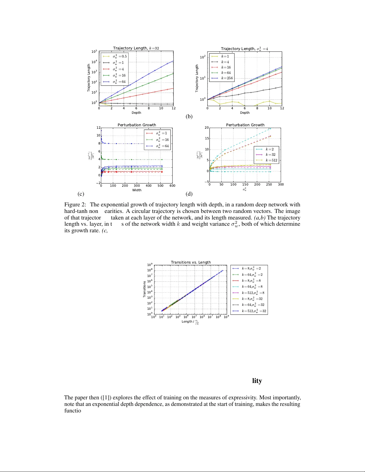
Surv ey of Expr essivity in Deep Neural Netw orks Maithra Raghu Google Brain and Cornell Univ ersity Ben Poole Stanford Univ ersity and Google Brain Jon Kleinberg Cornell Univ ersity Surya Ganguli Stanford Univ ersity Jascha Sohl-Dickstein Google Brain Abstract W e surve y results on neural network expressi vity described in [ 1 ]. The paper moti vates and de velops three natural measures of expressi veness, which all display an exponential dependence on the depth of the network. In fact, all of these measures are related to a fourth quantity , trajectory length . This quantity grows exponentially in the depth of the network, and is responsible for the depth sensitivity observed. These results translate to consequences for networks during and after training. They suggest that parameters earlier in a network ha ve greater influence on its expressi v e power – i n particular , gi ven a layer , its influence on expressi vity is determined by the r emaining depth of the network after that layer . This is verified with experiments on MNIST and CIF AR-10. W e also explore the effect of training on the input-output map, and find that it trades off between the stability and expressi vity . 1 Motivation and Setting In this survey , we summarize results on the expr essivity of deep neural networks from [ 1 ]. Neural network expressi vity looks at ho w the architecture of the network (width, depth, connecti vity) affects the properties of the resulting function. Being a fundamental step to better understanding neural networks, there is much prior work in this area. Many of the existing results rely on comparing achievable functions of a particular network architecture, ([ 2 , 3 ], [ 4 , 5 , 6 , 7 ]). While compelling, these results also highlight limitations of much of the existing w ork on expressi vity – unrealistic assumptions are sometimes made about the architectural shape e.g. exponentially lar ge width, and networks are often compared via their ability to approximate one specific function, which, in isolation, cannot result in a more general conclusion. T o ov ercome this, we start by analyzing expressi veness in a setting which is both more general than one of hardcoded functions, and immediately related to practice – networks after r andom initialization. Not only does this mean conclusions are independent of specific weight settings, b ut understanding behavior at random initialization pro vides a natural baseline to compare to the ef fects of training and trained networks, which we summarize in Sections 3, 4. Companion Paper In a companion paper , [ 8 ], the propagation of Riemannian curvatur e through random networks is studied by dev eloping a mean field theory approach, which quantitativ ely supports the conjecture that deep networks can disentangle curved manifolds in input space. 2 Random networks The results on networks after random initialization examine the effect of depth and width of a network architecture on its e xpressi ve po wer after random initialization via three natural measures of functional richness, number of transitions, acti v ation patterns, and dichotomies. More precisely , fully connected networks of input dimension m , depth n and width k are studied, with weights, bias randomly initialized as ∼ N (0 , σ 2 w /k ) , N (0 , σ 2 b ) . -1 0 1 x 0 -1 0 1 x 1 Layer 0 -1 0 1 x 0 -1 0 1 Layer 1 -1 0 1 x 0 -1 0 1 Layer 2 Figure 1: Deep networks with piecewise linear activ ations subdivide input space into con ve x polytopes. Here we plot the boundaries in input space separating unit activ ation and inacti vation for all units in a three layer ReLU network, with four units in each layer . The left pane shows activ ation boundaries (corresponding to a hyperplane arrangement) in gray for the first layer only , partitioning the plane into regions. The center pane sho ws acti vation boundaries for the first two layers. Inside every first layer region, the second layer activ ation boundaries form a differ ent hyperplane arrangement. The right pane shows activ ation boundaries for the first three layers, with different hyperplane arrangements inside all first and second layer re gions. This final set of con vex regions correspond to different acti v ation patterns of the network – i.e. different linear functions. 2.1 Measures of Expressivity In more detail, the measures of expressi vity are: T ransitions: Counting neuron transitions is introduced indirectly via linear regions in [ 9 ], and provides a tractable method to estimate the non-linearity of the computed function. Activation Patterns: T ransitions of a single neuron can be extended to the outputs of all neurons in all layers, leading to the (global) definition of a network activation pattern , also a measure of non-linearity . Network activ ation patterns directly show ho w the network partitions input space (into con ve x polytopes ), through connections to the theory of hyperplane arrangements , Figure 1. Dichotomies: The heter og eneity of a generic class of functions from a particular architecture is also measured, by counting the number of dichotomies seen for a fixed set of inputs. This measure is ‘statistically dual’ to sweeping input in some cases. The paper sho ws that all three measures grow exponentially with the depth of the netw ork, but not with the width. Connection to T rajectory Length In fact, this is due to an underlying connection of all three measures to another quantity , trajectory length – ho w a 1-D curv e in input space changes in length as it propagates through the network. It is prov ed [ 1 ] that the trajectory length of an input gro ws exponentially in the depth of a network b ut not the width: Theorem 1. Bound on Growth of T rajectory Length Let F W be a har d tanh random neural network and x ( t ) a one dimensional trajectory in input space. Define z ( d ) ( x ( t )) = z ( d ) ( t ) to be the image of the trajectory in layer d of F W , and let l ( z ( d ) ( t )) = R t       dz ( d ) ( t ) dt       dt be the ar c length of z ( d ) ( t ) . Then E h l ( z ( d ) ( t )) i ≥ O      σ w ( σ 2 w + σ 2 b ) 1 / 4 · √ k q p σ 2 w + σ 2 b + k   d    l ( x ( t )) This is also verified empirically (Figure 2). Theoretical intuition is the pro vided for the dir ect pr oportionality of transitions, activ ation patterns and dichotomies to trajectory length, and is further confirmed through experiments ([1]). 2 (a) 0 2 4 6 8 10 12 Depth 1 0 0 1 0 1 1 0 2 1 0 3 1 0 4 1 0 5 Trajectory Length T r a j e c t o r y L e n g t h , k = 3 2 σ 2 w = 0 . 5 σ 2 w = 1 σ 2 w = 4 σ 2 w = 1 6 σ 2 w = 6 4 (b) 0 2 4 6 8 10 12 Depth 1 0 0 1 0 1 1 0 2 Trajectory Length T r a j e c t o r y L e n g t h , σ 2 w = 4 k = 1 k = 4 k = 1 6 k = 6 4 k = 2 5 6 (c) 0 100 200 300 400 500 600 Width 2 0 2 4 6 8 10 12 | | δ x d + 1 | | | | δ x d | | Perturbation Growth σ 2 w = 1 σ 2 w = 1 6 σ 2 w = 6 4 (d) 0 50 100 150 200 250 300 σ 2 w 5 0 5 10 15 20 | | δ x d + 1 | | | | δ x d | | Perturbation Growth k = 2 k = 3 2 k = 5 1 2 Figure 2: The exponential gro wth of trajectory length with depth, in a random deep network with hard-tanh nonlinearities. A circular trajectory is chosen between two random vectors. The image of that trajectory is taken at each layer of the network, and its length measured. (a,b) The trajectory length vs. layer, in terms of the network width k and weight v ariance σ 2 w , both of which determine its growth rate. (c,d) The av erage ratio of a trajectory’ s length in layer d + 1 relativ e to its length in layer d . The solid line shows simulated data, while the dashed lines sho w upper and lo wer bounds (Theorem 1). Growth rate is a function of layer width k , and weight variance σ 2 w . 1 0 0 1 0 1 1 0 2 1 0 3 1 0 4 1 0 5 1 0 6 1 0 7 1 0 8 1 0 9 L e n g t h / σ w p k 1 0 0 1 0 1 1 0 2 1 0 3 1 0 4 1 0 5 1 0 6 1 0 7 1 0 8 1 0 9 Transitions Transitions vs. Length k = 8 , σ 2 w = 2 k = 6 4 , σ 2 w = 2 k = 8 , σ 2 w = 8 k = 6 4 , σ 2 w = 8 k = 5 1 2 , σ 2 w = 8 k = 8 , σ 2 w = 3 2 k = 6 4 , σ 2 w = 3 2 k = 5 1 2 , σ 2 w = 3 2 Figure 3: The number of transitions is linear in trajectory length. Here we compare the empirical number of sign changes to the length of the trajectory , for images of the same trajectory at different layers of a hard-tanh network. W e repeat this comparison for a variety of network architectures, with different netw ork width k and weight v ariance σ 2 w . 3 The effect of T raining: T rading Off Expressivity and Stability The paper then ([ 1 ]) explores the effect of training on the measures of expressi vity . Most importantly , note that an exponential depth dependence, as demonstrated at the start of training, makes the resulting function very sensiti ve to perturbations, not a desired feature in a trained netw ork. When weights are initialized with large σ 2 w , training increases stability by reducing trajectory length and transitions during the training process (Figure 4). 3 0 2 4 6 8 10 12 Layer number 1 0 1 1 0 2 Trajectory Length MNIST inputs 0 2 4 6 8 10 12 Layer number Random inputs Trajectory Length during training Figure 4: T raining acts to stabilize the input-output map by decreasing trajectory length for σ w large. The left pane plots the growth of trajectory length as a circular interpolation between two MNIST datapoints is propagated through the network, at different train steps. Red indicates the start of training, with purple the end of training. Interestingly , and supporting the observ ation on remaining depth, the first layer appears to increase trajectory length, in contrast with all later layers, suggesting it is being primarily used to fit the data. The right pane sho ws an identical plot but for an interpolation between random points , which also display decreasing trajectory length, b ut at a slo wer rate. Note the output layer is not plotted, due to artificial scaling of length through normalization. The network is initialized with σ 2 w = 16 . A similar plot is observed for the number of transitions (see Appendix.) 0 2 4 6 8 10 12 Layer number 1 0 1 1 0 2 Trajectory Length MNIST inputs 0 2 4 6 8 10 12 Layer number Random inputs Trajectory Length during training Figure 5: Training increases e xpressivity of input-output map for σ w small. The left pane plots the growth of trajectory length as a circular interpolation between two MNIST datapoints is propag ated through the network, at different train steps. Red indicates the start of training, with purple the end of training. W e see that the training process increases trajectory length, likely to increase the expressi vity of the input-output map to enable greater accurac y . The right pane sho ws an identical plot but for an interpolation between random points , which also displays increasing trajectory length, but at a slo wer rate. Note the output layer is not plotted, due to artificial scaling of length through normalization. The network is initialized with σ 2 w = 3 . When the network is initialized with too small a σ 2 w howe v er , this also has the potential to adversely affect performance as the function at initialization might not of fer enough e xpressiv eness to fit the target. In this case, we see that the training process monotonically incr eases the trajectory length and number of transitions (Figure 5.) In summary , the paper [ 1 ] concludes that training trades off between achie ving enough e xpressiv eness and simultaneously trying to maintain stability . 4 T rained Networks: Po wer of Remaining Depth The expanding trajectory length suggests that the ef fect of parameter choices earlier in earlier layers is amplified by later layers. Combining this with the exponential increase in dichotomies with depth, this suggests that the expressi ve po wer of the parameters, and thus layers, is related to the r emaining depth of the network after that layer . The paper demonstrates this in practice, with e xperiments on MNIST and CIF AR-10 (Figure 6). 4 0 100 200 300 400 500 Epoch Number 0.3 0.4 0.5 0.6 0.7 0.8 0.9 1.0 Accuracy Train Accuracy Against Epoch 0 100 200 300 400 500 Epoch Number Test Accuracy Against Epoch lay 2 lay 3 lay 4 lay 5 lay 6 lay 7 lay 8 lay 9 Figure 6: Demonstration of expressi ve po wer of remaining depth on MNIST . Here we plot train and test accuracy achie ved by training exactly one layer of a fully connected neural net on MNIST . The different lines are generated by varying the hidden layer chosen to train. All other layers are kept frozen after random initialization. References [1] Maithra Raghu, Ben Poole, Jon Kleinber g, Surya Ganguli, and Jascha Sohl-Dickstein. On the expressiv e power of deep neural netw orks. ArXiv e-prints , June 2016. URL . [2] Kurt Hornik, Maxwell Stinchcombe, and Halbert White. Multilayer feedforward networks are univ ersal approximators. Neural networks , 2(5):359–366, 1989. [3] George Cybenko. Approximation by superpositions of a sigmoidal function. Mathematics of contr ol, signals and systems , 2(4):303–314, 1989. [4] Ronen Eldan and Ohad Shamir . The power of depth for feedforward neural networks. arXiv pr eprint arXiv:1512.03965 , 2015. [5] Matus T elgarsky . Representation benefits of deep feedforward networks. arXiv pr eprint arXiv:1509.08101 , 2015. [6] James Martens, Arkadev Chattopadhya, T oni Pitassi, and Richard Zemel. On the representational efficienc y of restricted boltzmann machines. In Advances in Neur al Information Pr ocessing Systems , pages 2877–2885, 2013. [7] Monica Bianchini and Franco Scarselli. On the complexity of neural network classifiers: A comparison between shallow and deep architectures. Neural Networks and Learning Systems, IEEE T r ansactions on , 25 (8):1553–1565, 2014. [8] Ben Poole, Subhaneil Lahiri, Maithra Raghu, Jascha Sohl-Dickstein, and Surya Ganguli. Exponential expressi vity in deep neural networks through transient chaos. In Advances In Neural Information Pr ocessing Systems , pages 3360–3368, 2016. [9] Razvan P ascanu, Guido Montufar , and Y oshua Bengio. On the number of response regions of deep feed forward networks with piece-wise linear acti v ations. arXiv preprint , 2013. 5