Learning From Graph Neighborhoods Using LSTMs

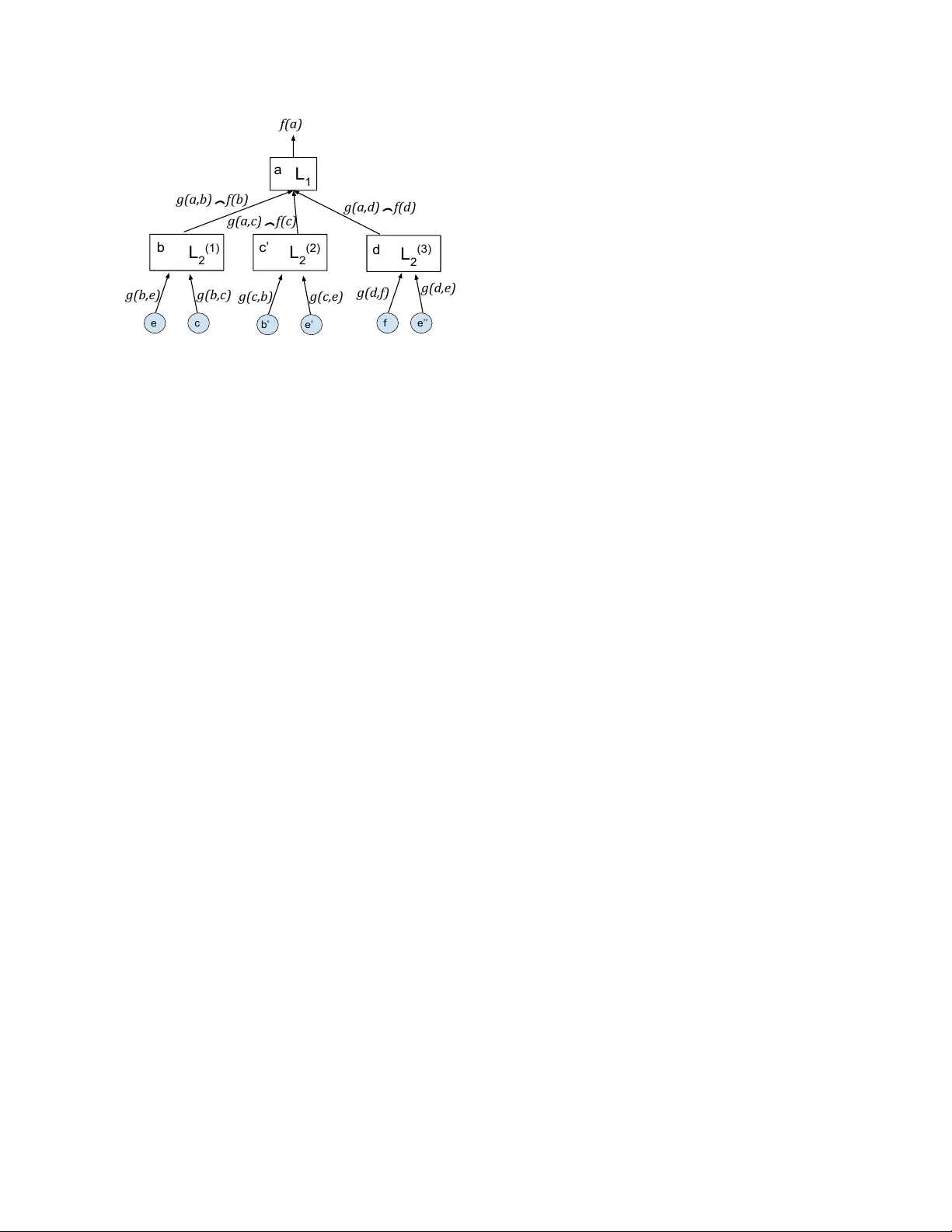
Learning From Graph Neighborhoods Using LSTMs Rakshit Agraw al ∗ Luca de Alfaro V assilis Polychronopoulos ragraw a1@ucsc.edu, luca@ucsc.edu, v assilis@cs.ucsc.edu Computer Science Department, Uni versity of California, Santa Cruz T echnical Report UCSC-SOE-16-17 School of Engineering, UC Santa Cruz Nov ember 18, 2016 Abstract Many prediction problems can be phrased as inferences ov er local neighborhoods of graphs. The graph repre- sents the interaction between entities, and the neighbor- hood of each entity contains information that allows the inferences or predictions. W e present an approach for ap- plying machine learning directly to such graph neighbor- hoods, yielding predicitons for graph nodes on the basis of the structure of their local neighborhood and the fea- tures of the nodes in it. Our approach allows predictions to be learned directly from examples, bypassing the step of creating and tuning an inference model or summarizing the neighborhoods via a fix ed set of hand-crafted features. The approach is based on a multi-lev el architecture built from Long Short-T erm Memory neural nets (LSTMs); the LSTMs learn how to summarize the neighborhood from data. W e demonstrate the effecti veness of the proposed technique on a synthetic example and on real-world data related to crowdsourced grading, Bitcoin transactions, and W ikipedia edit re versions. 1 Intr oduction Many prediction problems can be naturally phrased as inference problems ov er the local neighborhood of a graph. Consider , for instance, crowdsourced grading. W e can construct a (bipartite) graph consisting of items and graders, where edges connect items to users who graded them, and are labeled with the grade assigned. T o in- fer the grade for an item, we can look at the graph in- volving the adjacent nodes: this graph, known as the 1- neighborhood, consists of the people who graded the item ∗ The authors prefer to be listed in alphabetical order . and of the grades they assigned. If we wish to be more so- phisticated, and try to determine which of these people are good graders, we could look also at the work performed by these people, expanding our analysis outwards to the 2- or 3-neighborhood of each item. For another example, consider the problem of predict- ing which bitcoin addresses will spend their deposited funds in the near future. Bitcoins are held in “addresses”; these addresses can participate in transactions where they send or receive bitcoins. T o predict which addresses are likely to spend their bitcoin in the near future, it is natural to build a graph of addresses and transactions, and con- sider neighborhoods of each address. The neighborhood contains information on where the bitcoins came from, and on what happened to bitcoins at the interacting ad- dresses, which (as we will show) can help predict whether the coins will be transacted soon. For a third example, consider the problem of predicting user behavior on W ikipedia. Users interact by collabora- tiv ely editing articles, and we are interested in predicting which users will hav e their work reverted. W e can build a graph with users as nodes, and interactions as edges: an interaction occurs when two users edit the same article in short succession, and one either keeps, or undoes, the work of the other . The 1-neighborhood of a user will tell us how often that user’ s work has been kept or re verted. Again, we can consider lar ger neighborhoods to gather information not only on the user , b ut on the people she in- teracted with, trying to determine whether they are good contributors, how experienced they are, whether they are in v olved in an y disputes, and so forth. In this paper , we show how to solve these problems by applying machine learning, using an architecture based on multi-lev el Long Short-T erm Memory (LSTM) neural nets [14, 9, 10], with each LSTM le vel processing one “degree 1 of separation” in the neighborhood. The challenge of applying machine learning to graph neighborhoods lies in the fact that many common machine learning methods, from neural nets [15] to support vector machines (SVMs) [6], are set up to handle fixed-length vectors of features as input. As a graph neighborhood is variable in size and topology , it is necessary to summarize the neighborhood into a fixed number of features to use in learning. Some machine learning methods, such as lo- gistic regression [5], can accept a potentially unbounded number of inputs, but ev ery input has its o wn index or name, and it is not ob vious ho w to map the local topology of a graph into such fixed naming scheme in a way that preserves the structure, or the useful information. Machine-learning methods that can learn from se- quences, such as LSTMs or recurrent neural nets [26, 13], offer more power . It is possible to trav erse the local neigh- borhood of a node in a graph in some order (pre-, post-, or in-order), and encode the neighborhood in a sequence of features complete with markers to denote edge traver - sals, and then feed this sequence to an LSTM. W e ex- perimented with this approach, but we did not obtain any useful results: the LSTMs were unable to learn anything useful from a flattened presentation of the graph neigh- borhood. W e propose a learning architecture based on the use of multiple le vels of LSTMs. Our architecture performs predictions for one “target” graph node at a time. First, the graph is unfolded from the tar get node, yielding a tree with the target node as its root at lev el 0, its neighbors as lev el-1 children, its neighbors’ neighbors as le vel-2 chil- dren, and so forth, up to a desired depth D . At each tree node v of le vel 0 ≤ d < D , a lev el- d + 1 LSTM is fed sequentially the information from the children of v at level d + 1 , and produces as output information for v itself. Thus, we exploit LSTMs’ ability to process se- quences of any length to process trees of any branching factor . The top-level LSTM produces the desired predic- tion for the target node. The architecture requires training D LSTMs, one per tree lev el. The LSTMs learn how to summarize the neighborhood up to radius D on the basis of data, av oiding the manual task of synthesizing a fixed set of features. By dedicating one LSTM to each lev el, we can tailor the learning (and the LSTM size) to the distance from the target node. For instance, in the bipartite graph arising from cro wdsourced grading, it is desirable to use different LSTMs for aggregating the edges con verging to an item (representing grades receiv ed), and for aggregat- ing the edges con verting to a user (representing the grades assigned). W e demonstrate the effecti veness of the proposed ap- proach over four problems. The first problem is a syn- thetic example concerning the crowdsourcing of yes/no labels for items. The other three are based on real data, and they are the previously mentioned problems of ag- gregating cro wdsourced grades, predicting bitcoin spend- ing, and predicting future reversions of user’ s edits in W ikipedia. In all four problems, we show that the ability of MLSL to exploit any feature in the data leads to high performance with minimal feature engineering effort and no apriori model assumptions. W e are making available the open-source code implementing LSTMs and MLSL, along with the datasets, at https://sites.google. com/view/ml- on- structures . 2 Related W ork Predicting properties of nodes in graph structures is a common problem that has been widely studied. Sev eral existing approaches view this as a model-based inference problem. A model is created, and its parameters are tuned on the basis of the information av ailable; the model is then used to perform inference. As the exact probabilistic in- ference is generally intractable [18], most techniques rely on iterati ve approximation approaches. Iterative approxi- mations are also at the root of expectation maximization (EM) [7]. Iterativ e parameter estimation has been used, together with Gibbs sampling, to reliably aggregate peer grades in massive on-line courses [22]. Iterativ e, model- based approaches hav e also been used for reliably crowd- sourcing boolean or multi-class labels [16, 17]. In these works, a bipartite graph of items and workers is created, and then the work er reliabilities, and item labels or grades, are iterativ ely estimated until conv ergence. Compared to these models, the benefit of our proposed approach is that it does not require a model, and thus, it can av ail itself of all the features that happen to be avail- able. For instance, in crowdsourced grading, we can use not only the agreement among the graders to judge their reliability , but also any other information that might be av ailable, such as the time taken to grade, or the time of day , or the number of items previously graded by the user , without need to hav e a model of ho w these features might influence grade reliability . W e will show that this abil- ity can lead to superior performance compared to EM and [16] when additional features are available. On the other hand, machine-learning based approaches such as ours are dependent on the av ailability of training data, while model-based approaches can be employed even in its ab- sence. Sev eral approaches have been proposed for summariz- ing graph structures in feature vectors. The algorithm 2 node2vec [12] enables the construction of feature vec- tors for graph nodes in such a way that the feature vec- tor optimally represents the node’ s location in the graph. Specifically , the feature v ector maximizes the a-posteriori probability of graph neighborhoods gi ven the feature vec- tor . The resulting feature v ector thus summarizes a node’ s location in a graph, but it does not summarize the origi- nal features of the node, or of its neighbors. In contrast, the techniques we introduce allo w us to feed to machine learning the node features of an entire graph neighbor - hood. In DeepW alk [21], feature vectors for graph nodes are constructed by performing random walks from the nodes, and applying them various summarization techniques to the list of feature vectors of the visited nodes. This approach enables the consideration of variable-diameter neighborhoods, in contrast to our exploration, which pro- ceeds strictly breath-first. In DeepW alk, the construction of the summarizing feature vector proceeds according to a chosen algorithm, and is not guided by backpropagation from the learning goal. In other words, the summariza- tion is not learned from the ov erall ML task. In contrast, in our approach the summarization itself, carried out by the LSTMs, is learned via backpropagation from the goal. LSTMs were proposed to overcome the problem of vanishing gradient o ver long sequences problems with re- current neural nets [14, 9]; they have been widely useful in a wide variety of learning problems; see, e.g., [11, 23]. Recurrent neural nets and LSTMs hav e been generalized to multi-dimensional settings [4, 10]. The multi-level ar- chitecture proposed here can handle arbitrary topologies and non-uniform nodes and edges (as in bipartite graphs), rather than regular n-dimensional lattices, at the cost of exploring smaller neighborhoods around nodes. Learning over graphs can be reduced to a standard machine-learning problem by summarizing the informa- tion av ailable at each node in a fixed set of features. This has been done, for instance, with the goal of link predic- tion, consisting in predicting which users in a social net- work will collaborate or connect next [3]. Graph summa- rization typically requires deep insight into the problem, in order to design the summary features. The multi-lev el LSTMs we propose here constitute a way of learning such graph summarization. Some recent work has looked at the problem of sum- marizing very large graphs into feature vectors [24]. The goals (and methods) are thus different from those in the present paper , where the emphasis consists in considering nodes together with their immediate neighborhoods as in- put to machine learning. There is much work on learning with graphs, where the graph edges encode the similarity between the nodes (rather than features, as in our case); see, e.g., [28, 8]. This represents an interesting, b ut orthogonal application to ours. 3 Learning fr om Graph Neighbor - hoods W e consider a graph G = ( V , E ) with set of vertices V and edges E ⊆ V × V . W e assume that each edge e ∈ E is labeled with a vector of features g ( e ) of size M . Each verte x v ∈ V is associated with a vector of labels. The goal is to learn to predict the verte x labels on the basis of the structure of the graph and the edge labels. This setting can model a wide v ariety of problems. Considering only edge features, rather than also vertex features, in volves no loss of generality: if there are inter- esting features associated with the vertices, they can be in- cluded in the edges leading to them. If the goal consists in predicting edge outputs, rather than vertex, one can con- struct the dual graph G 0 = ( E , V 0 ) of G , where edges of G are vertices of G 0 , and where V 0 = { (( u, v ) , ( v , w )) | ( u, v ) , ( v , w ) ∈ E } . Learning method overview . Our learning strategy can be summarized as follo ws. In order to predict the label of a node v , we consider the tree T v rooted at v and with depth D , for some fixed D > 0 , obtained by unfolding the graph G starting from v . W e then traverse T v bottom- up, using sequence learners, defined below , to compute a label for each node from the labels of its children edges and nodes in T v . This trav ersal yields an output label y v for the root v of the tree. In training, the output y v can be compared with the desired output, a loss be computed, and backpropagated through the tree. W e now present in detail these steps. Graph unfolding. Giv en the graph G = ( V , E ) and a node v ∈ V , along with a depth D > 0 , we define the full unfolding of G of depth D at v as the tree T v with root v , constructed as follows. The root v has depth 0 in T v . Each node u of depth k < D in T v has as children in T v all nodes z with ( u, z ) ∈ E ; the depth of each such z is one plus the depth of u . A single graph node may correspond to more than one node in the unfolding. W e will rename the nodes of the unfolding so that they are all distinct; nodes and edges in the unfolding inherit their labels from their correspondents in the graph. It is possible to perform learning using asymmetric un- folding, in which if a node u has parent u 0 , we let the 3 a b c d b e’ b’ c’ d a e c e e’’ f f Figure 1: An example of a graph and its asymmetric un- folding at node a for depth 2 . W e rename the nodes that appear in man y locations so that the y ha ve distinct names, for instance, we use e , e 0 and e 00 to denote the copies of e . descendants of u be { z | ( u, z ) ∈ E , z 6 = u 0 } . Figure 1 il- lustrates a graph and its asymmetric tree unfolding at node a and depth 2. Which of the two unfolding is more useful depends on the specifics of the learning problem, and we will discuss this choice in our applications. Sequence learners. Our proposed method for learn- ing on graphs lev erages sequence learners. A sequence learner is a machine-learning algorithm that can accept as input an arbitrary-length sequences of feature vectors, producing a single vector as output. Long Short-T erm Memory neural nets (LSTMs) [14] are an example of such sequence learners. W e denote a sequence learner parame- terized by a vector w of parameters by L [ w ] . In LSTMs, the parameter vector w consists of the LSTM weights. W e say that a sequence l earner is of shape ( N , K ) if it accepts a sequence of vectors of size N , and produces a vector of size K as output. W e assume that a sequence learner L [ w ] of shape ( N , K ) can perform three operations: • F orward pr opagation. Gi ven a input sequence x (1) , x (2) , . . . , x ( n ) , where each x ( i ) is a vector of size N , compute an output y , where y is a vector of size K . • Loss backpr opagation. For a loss function L , gi ven ∂ L /∂ y for the output, it can compute ∂ L /∂ x ( j ) for each x (1) , x (2) , . . . , x ( N ) . Here, ∂ L /∂ y is a vector having ∂ L /∂ y i as component for each component y i of y , and like wise, ∂ L /∂ x ( j ) is a vector with com- ponents ∂ L /∂ x ( j ) k , for each component x ( j ) k of x ( j ) . • P arameter update. For a loss function L , giv en ∂ L /∂ y for the output, it can compute a vector ∆ w of parameter updates. The parameter updates can be for instance computed via a gradient-descent method, taking ∆ w = − α∂ L /∂ w for some α > 0 , but the precise method varies according to the structure of the sequence learner; see, e.g., [9]. In an LSTM, backpropagation and parameter update are performed via bac kpropa gation thr ough time; see [25, 26] for details. 3.1 Multi-Lev el Sequence Learners Giv en a graph G with labeled edges as above, we now describe the learning architecture, and how to perform the forward step of node label prediction, and the backward step of backpropagation and parameter updates. W e term our proposed architecture multi-level sequence learners, or MLSL, for short. 1 W e start by choosing a fixed depth D > 0 for the un- folding. The prediction and learning is performed via D sequence learners L 1 , L 2 , . . . , L D . Each sequence learner L i will be responsible for aggregating information from children at depth i in the unfolding trees, and computing some information for their parent, at depth i − 1 . The se- quence learner L D has shape ( M , K D ) , where M is the size of the edge labels: from the edge labels, it computes a set of features of size K D . For each 0 < d < D , the se- quence learner at depth d has shape ( M + K d +1 , K d ) for some K d > 0 , so that it will be able to aggregate t he edge labels and the output of the learners belo w , into a single vector of size K d . Note that learners L d for depth 1 < d ≤ D can appear multiple times in the tree, once for each node at depth d − 1 in the tree. All of these instances of L d share the same parameters, but are treated separately in forward and backward propagation. The behavior of these sequence learners is defined by the parameter vectors w (1) , . . . , w ( D ) ; the goal of the learning is to learn the values for these parameter vectors that minimizes the loss function. W e stress that the se- quence learners L 1 , L 2 , . . . , L D and their parameter vec- tors w (1) , . . . , w ( D ) can depend on the depth in the tree (there are D of them, indeed), but they do not depend on the root node v whose label we are trying to predict. In order to learn, we repeatedly select root nodes v ∗ ∈ V , for instance looping o ver them, or via some probability distribution ov er nodes, and we construct the unfoldings T v ∗ . W e then perform over T v ∗ the forward and backprop- agation steps, and the parameter update, as follo ws. Forward propagation. The forward propagation step proceeds bottom-up along T v . Figure 2 illustrates how the sequence learners are applied to an unfolding of the root node a of the graph of Figure 1 with depth 2 to yield a prediction for node a . • Depth D . Consider a node v of depth D − 1 with children u 1 , . . . , u k at depth D . W e use the sequence 1 Open-source code implementing MLSL will be made av ailable by the authors. 4 L 1 L 2 (1) f(a) g(a,b) ⁀ f(b) g(a,c) ⁀ f(c) g(a,d) ⁀ f(d) g(c,b) g(c,e) L 2 (2) L 2 (3) b’ e’ g(b,e) g(b,c) e c g(d,f) g(d,e) f e’’ b c’ d a Figure 2: Forward propagation corresponding to the tree unfolding of Figure 1. The elements of the sequence which is fed to learner L 1 consist of the features of the respectiv e edges concatenated with the output from learn- ers below . Note the use of three instances of the learner L 2 , one for each depth-2 node in the unfolding. These instances share the same parameters. In the figure, the symbol _ denotes the concatenation of feature vectors. learner L D to aggregate the sequence of edge labels g ( v , u 1 ) , . . . , g ( v , u k ) into a single label f ( v ) for v . • Depth 0 < d < D . Consider a node v at depth d − 1 with children u 1 , . . . , u k at depth d . W e forward to the learner L d the sequence of vec- tors g ( v , u 1 ) _ f ( u 1 ) , . . . , g ( v , u n ) _ f ( u n ) obtained by concatenating the feature vectors of the edges from v to the children, with the feature vectors com- puted by the learners at depth d + 1 . The learner L d will produce a feature vector f ( v ) for v . Backward propagation. Once we obtain a vector y = f ( v ∗ ) for the root of T v ∗ , we can compute the loss L ( y ) , and we can compute ∂ L /∂ y . This loss is then backprop- agated from the root down to the lea ves of T v ∗ , following the topology of the tree (refer again to Figure 2). Con- sider a node v at depth d − 1 , for 0 < d ≤ D , with computed feature vector f ( v ) . W e backpropagate through the instance of the learner L d that computed f ( v ) the loss, obtaining ∂ L /∂ x i for the input vectors x (0) , . . . , x ( k ) cor- responding to the children u 1 , . . . , u k of v . • If these children are at depth d < D , each vector x ( j ) consists of the concatenation g ( v , u j ) _ f ( u j ) of the features g ( v , u j ) from the graph edge, and of the features f ( u j ) computed for u j . As the former re- quire no further backpropagation, we retain the por- tion ∂ L /∂ f ( u j ) for further backpropagation. • At the bottom depth d = D of the tree, each vector x ( j ) corresponds to the graph edge labels g ( v , u j ) , and backpropagation terminates. Parameter update (learning). Consider a learner L d for depth 1 ≤ d ≤ D , defined by parameters w ( d ) . T o update the parameters w ( d ) , we consider all instances L (1) d , . . . , L ( m ) d of L d in the tree T v ∗ , corresponding to the nodes v 1 , . . . , v m at depth d (refer again to Figure 2). For each instance L ( i ) d , for i = 1 , . . . , m , from ∂ L /∂ f ( v i ) we can compute a parameter update ∆ i w ( d ) . W e can then compute the overall parameter update for L d as the av er- age ∆ w ( d ) =  ∆ 1 w ( d ) + · · · + ∆ m w ( d )  /m of the updates ov er the individual instances. Preser ving learner instance state. As mentioned abov e, a sequence learner for a given depth may occur in several instances in the tree obtained by unfolding the graph (see Figure 1). Commonly , to perform backprop- agation and parameter update though a learner , it is nec- essary to preserve (or recompute) the state of the learner after the forward propagation step; this is the case, for in- stance, both for neural nets and for LSTMs. Thus, ev en though all learner instances for depth d are defined by a single parameter vector w ( d ) , it is in general necessary to cache (or reconstruct) the state of every learner instance in the tree individually . 3.2 T raining During training, we repeatedly select a target node, unfold the graph, feed the unfolding to the multi-lev el LSTMs, obtain a prediction, and backpropagate the loss, updating the LSTMs. An important choice is the order in which, at each tree node, the edges to children nodes are fed to the LSTM. The edges can be fed in random order , shuffling the order for e very training sample, or they can be fed in some fix ed order . In our applications, we ha ve found each of the two approaches to ha ve uses. 4 A pplications W e have implemented multi-le vel sequence learners on the basis of an LSTM implementation performing backpropagation-though-time learning [10], which we combined with an AdaDelta choice of learning step [27]. W e report the results on one synthetic setting, and three case studies based on real data. The code and the datasets can be found at https://sites.google. com/view/ml- on- structures . 5 For imbalanced datasets, apart from the accuracy (per- centage of correct guesses), we report the av erage re- call, which is the unweighted av erage of the recall of all classes. This is suitable in the case of classes of differ - ent frequencies, since for highly imbalanced datasets it is easy to inflate the accuracy measure by predicting labels of the most frequent classes. 4.1 Cro wdsourcing boolean labels W e considered the common boolean crowdsourcing task where users provide yes/no labels for items. This is mod- eled as a bipartite graph, with items and users as the two kind of nodes; the edges are labeled with yes/no. The task consists in reconstructing the most likely labels for the items. W e generated synthetic data similar to the one used in [16]. In the data, items have a true yes/no la- bel (which is not visible to the inference algorithms), and users have a hidden boolean variable indicating whether they are truthful, or random. Truthful users report the item label, while random users report yes/no with prob- ability 0 . 5 each. This is also called the spammer-hammer user model. W e report results for a graph of 3000 users and 3000 items where item labels are balanced (50% yes/ 50% no) and the probability of a user being reliable is 60%. Each item gets 3 votes from dif ferent users. W e compare three algorithms: • The iterativ e algorithm of [16], abbreviated as KOS. The algorithm requires no prior . • Expectation Maximization (EM) [7], where user re- liability is modeled via a beta distribution. W e used an informativ e prior (shape parameters α = 1 . 2 and β = 1 . 0 ) for the initial beta distribution which re- flects the proportion of reliable users in the graph. • Our multi-lev el sequence learners with depths 1 and 3, denoted 1-MLSL and 3-MLSL, where the output (and memory) sizes of 3-MLSL are K 2 = K 3 = 3 . W e train on 1 , 000 items and test on the remaining 2 , 000 . For multi-level LSTM, we also consider the case where users hav e an additional observable feature that is corre- lated to their truthfulness. This represents a feature such as “the user created an account over a week ago”, which is observable, but not part of standard crowdsourcing mod- els. This feature is true for 90% of reliable users and for for 40% of unreliable users. W e denote the algorithms that hav e access to this extra feature as 1-LSL+ and 3-LSL+; K OS and EM cannot make use of this feature as it is not part of their model. Our intent is to sho w ho w machine- learning approaches such as MLSLs can increase their Method Accuracy K OS 0.8016 EM 0.9136 Method Accuracy 1-MLSL 0.8945 3-MLSL 0.9045 1-MLSL+ 0.9565 3-MLSL+ 0.9650 T able 1: Performance of K OS [16], EM (Expectation Maximization) and multi-lev el sequence learners (ML- SLs) of different depths. performance by considering additional features, indepen- dently of a model. W e report the results in T able 1. When no additional information is av ailable, EM is superior to 1-MLSL and slightly superior to 3-MLSL. When the additional feature is av ailable, both 1-MLSL+ and 3-MLSL+ learn its use- fulness, and perform best. 4.2 Peer Grading W e considered a dataset containing peer grading data from computer science classes. The data comes from an online tool that lets students submit homework and grade each other’ s submissions. Each sumission is typically re- viewed by 3 to 6 other students. The data is a bipartite graph of users and submissions, as in the previous cro wd- sourcing application. Users assign grades to items in a predefined range (in our case, all grades are normalized in the 0-10 range). Each edge is labeled with the grade, and with some additional features: the time when the student started grading the submission, and the time when they submitted the grade. W e treat this as a classification task, where the classes are the integer grades 0, 1, . . . , 10; the ground trut h is pro vided by instructor grades, a vailable on a subset of submissions. Our dataset contined 1,773 la- beled (instructor-graded) submissions; we used 1,500 for training and 273 for testing. W e compare three methods. One is simple av erage of provided grades, rounded to the closest integer . Another method is based on expectation maximization (EM), iter- ativ ely learning the accuracy of users and estimating the grades. Finally , we employed MLSL with the following features (derived from the graph): the time to complete a revie w , the amount of time between revie w completion and revie w deadline, and the median grade received by the student in the assignment. The output of the learner at lev el 2 is of size 3 where it reaches its peak for this experiment. T able 2 shows the results. The 1- and 2-depth MLSL methods are superior to both the EM-based approach and av erage. A verage recall appears low due to the very 6 Method Accuracy A verage Recall A verage 0.5432 0.3316 EM-based 0.5662 0.3591 1-MLSL 0.6044 0.3897 2-MLSL 0.6010 0.3913 T able 2: Performance of EM and 1,2-depth MLSL on peer grading data. high class imbalance of the dataset: some low homework grades are very rare, and mistakes in these rare grades hav e high impact. 4.3 Prediction of Wikipedia Reversions W ikipedia is a popular crowdsourced knowledge reposi- tory with contributions from people all around the world and in various languages. Users occasionally add con- tributions that are re verted by other users, either due to their low quality , or as part of a quarrel, or simply due to carelessness. Our interest is in predicting, for each user , whether the user’ s next edit will be rev erted. W e note that this is a dif ferent (and harder) question than the ques- tion of whether a specific edit, whose features are already known, will be re verted in the future [2]. W e model the user interactions in W ikipedia as a multi- graph with users as nodes. An edge e from u 2 to u 1 rep- resents a “implicit interaction” of users u 2 and u 1 , occur- ring when u 2 creates a revision r 2 immediately following a revision r 1 by u 1 . Such an edge e is labeled with a feature vector consisting of the edit distances d ( r 1 , r 2 ) , d ( r 0 , r 2 ) and d ( r 0 , r 1 ) , where r 0 is the revision immedi- ately preceding r 1 , and d ( · ) is edit distance. The feature vector contains also the elapsed times between the re vi- sions, and the quality of r 1 measured from r 2 , defined by d ( r 0 , r 1 ) /  d ( r 0 , r 2 ) − d ( r 1 , r 2 )  [1]. Since the English W ikipedia has a very large dataset, for this experiment we used the complete dumps of the Asturian W ikipedia (Asturian is a language in Spain). The graph consists of o ver 32 , 000 nodes (users) and o ver 45 , 000 edge (edits among users). T o obtain the labels for each user , we consider the state of this graph at a time 30 days before the last date of content a vailable in the dump; this leaves ample time for rev ersions to occur in the extra 30 days, ensuring that we label users correctly . T o train the model, we repeatedly pick an edit by a user, and we construct the graph neighborhood around the user consist- ing only of the edits preceding the selected edit (we want to predict the future on the basis of the past). W e label the user with yes/no, according to whether the selected edit was re verted, or not. This local neighborhood graph A verage F-1 F-1 Recall rev erted not reverted 1-MLSL 0.8468 0.8204 0.8798 2-MLSL 0.8485 0.8259 0.8817 3-MLSL 0.8508 0.8288 0.8836 T able 3: Prediction of re versions in the Asturian W ikipedia, using MLSL of depths 1, 2, 3. is then fed to the MLSL. W e performed training on 60% of the data and validated with the remaining 40%. W e trained ov er 30 models for each depth and validated them by measuring the average recall and F1-scores for both labels. T able 3 shows the av erage results for each depth lev el. W e observ e that F-1 scores for both “rev ersion” and “no re version” labels were high. Moreo ver , these results show impro vement in performance for increasing depth. 4.4 Prediction of Bitcoin Spending The blockchain is the public immutable distributed ledger where Bitcoin transactions are recorded [20]. In Bitcoin, coins are held by addresses, which are hash values; these address identifiers are used by their o wners to anon y- mously hold bitcoins, with ownership prov able with pub- lic key cryptography . A Bitcoin transaction inv olves a set of source addresses, and a set of destination addresses: all coins in the source addresses are gathered, and they are then sent in various amounts to the destination addresses. Mining data on the blockchain is challenging [19] due to the anonymity of addresses. W e use data from the blockchain to predict whether an address will spend the funds that were deposited to it. W e obtain a dataset of addresses by using a slice of the blockchain. In particular , we consider all the addresses where deposits happened in a short range of 101 blocks, from 200,000 to 200,100 (included) . They contain 15,709 unique addresses where deposits took place. Looking at the state of the blockchain after 50,000 blocks (which cor- responds to roughly one year later as each block is mined on average ev ery 10 minutes), 3,717 of those addresses still had funds sitting: we call these “hoarding addresses”. The goal is to predict which addresses are hoarding ad- dresses, and which spent the funds. W e randomly split the 15,709 addresses into a training set of 10,000 and a validation set of 5,709 addresses. W e built a graph with addresses as nodes, and transac- tions as edges. Each edge w as labeled with features of the transaction: its time, amount of funds transmitted, num- ber of recipients, and so forth, for a total of 9 features. W e compared two dif ferent algorithms: • Baseline: an informativ e guess; it guesses a label 7 Accuracy A vg. Recall F-1 ‘spent’ F-1 ‘hoard’ Baseline 0.6325 0.4944 0.7586 0.2303 1-MLSL 0.7533 0.7881 0.8172 0.6206 2-MLSL 0.7826 0.7901 0.8450 0.6361 3-MLSL 0.7731 0.7837 0.8367 0.6284 T able 4: The prediction results on blockchain addresses using baseline approach, and MLSL of depths 1, 2, 3. with a probability equal to its percentage in the train- ing set. • MLSL of depths 1, 2, 3. The outputs and mem- ory sizes of the learners for the reported results are K 2 = K 3 = 3 . Increasing these to 5 maintained vir- tually the same performance while increasing train- ing time. Using only 1 output and memory cell was not providing an y advances in performance. T able 4 sho ws the results. Using the baseline we get poor results; the F-1 score for the smaller class (the ‘hoarding’ addresses) is particularly low . T apping the transaction history and using only one le vel the learner al- ready provides a good prediction and an a verage recall ap- proaching 80%. Increasing the number of le vels from 1 to 2 enhances the quality of the prediction as it digests more information from the history of transactions. Increasing the lev els beyond 2 does not lead to better results, with this dataset. 4.5 Discussion The results from the above applications show that MLSL can provide good predictive performance over a wide va- riety of problems, without need for de vising application- tailored models. If sufficient training data is av ailable, MLSL can use the graph representation of the problem and any a vailable features to achie ve high performance. One of our conclusions is that the order of processing the nodes during training matters. In crowdsourced grad- ing, randomly shuffling the order of edges for a learning instance as it is used in different iterations during the train- ing process, was superior to using a fixed order . For Bit- coin, on the other hand, feeding edges in temporal order worked best. This seems intuiti ve, as the transactions hap- pened in some temporal order . One challenge was the choice of learning rates for the various lev els. As the gradient backpropagates across the multiple levels of LSTMs, it becomes progressiv ely smaller . T o successfully learn we needed to use dif ferent learning rates for the LSTMs at dif ferent lev els, as the top lev els will tend to learn faster . Refer ences [1] B. Thomas Adler and Luca De Alfaro. A content- driv en reputation system for the W ikipedia. In Pr o- ceedings of the 16th international confer ence on W orld W ide W eb , pages 261–270. A CM, 2007. [2] B. Thomas Adler, Luca De Alfaro, Santiago M. Mola-V elasco, Paolo Rosso, and Andrew G. W est. W ikipedia vandalism detection: Combining natu- ral language, metadata, and reputation features. In Computational linguistics and intelligent text pr o- cessing , pages 277–288. Springer , 2011. [3] Mohammad Al Hasan, V ineet Chaoji, Saeed Salem, and Mohammed Zaki. Link prediction using super- vised learning. In SDM06: workshop on link analy- sis, counter-terr orism and security , 2006. [4] Pierre Baldi and Gianluca Pollastri. The princi- pled design of large-scale recursiv e neural network architecturesdag-rnns and the protein structure pre- diction problem. Journal of Machine Learning Re- sear ch , 4(Sep):575–602, 2003. [5] Christopher M. Bishop. P attern r ecognition , volume 128. Springer, 2007. [6] Corinna Cortes and Vladimir V apnik. Support- vector networks. Machine learning , 20(3):273–297, 1995. [7] Arthur P . Dempster , Nan M. Laird, and Donald B. Rubin. Maximum likelihood from incomplete data via the EM algorithm. Journal of the r oyal statisti- cal society . Series B (methodological) , pages 1–38, 1977. [8] Eyal En Gad, Akshay Gadde, A. Salman A ves- timehr , and Antonio Ortega. Active learning on weighted graphs using adapti ve and non-adapti ve approaches. In 2016 IEEE International Confer - ence on Acoustics, Speech and Signal Processing (ICASSP) , pages 6175–6179. IEEE, 2016. [9] Felix A. Gers and Jrgen Schmidhuber . LSTM recur- rent networks learn simple conte xt-free and context- sensitiv e languages. Neur al Networks, IEEE T rans- actions on , 12(6):1333–1340, 2001. [10] Ale x Graves. Supervised Sequence Labelling with Recurr ent Neural Networks . PhD thesis, T echnishe Univ ersit ¨ at M ¨ unchen, 2012. 8 [11] Ale x Grav es and Jrgen Schmidhuber . Offline hand- writing recognition with multidimensional recurrent neural networks. In Advances in neural information pr ocessing systems , pages 545–552, 2009. [12] Aditya Grov er and Jure Leskov ec. Node2vec: Scal- able Feature Learning for Networks. In Pr oceed- ings of the 22Nd ACM SIGKDD International Con- fer ence on Knowledge Discovery and Data Mining , KDD ’16, pages 855–864, Ne w Y ork, NY , USA, 2016. A CM. [13] Sepp Hochreiter , Y oshua Bengio, Paolo Frasconi, and Jrgen Schmidhuber . Gradient flow in recurr ent nets: the difficulty of learning long-term dependen- cies . A field guide to dynamical recurrent neural net- works. IEEE Press, 2001. [14] Sepp Hochreiter and Jrgen Schmidhuber . Long short-term memory . Neural computation , 9(8):1735–1780, 1997. [15] John J. Hopfield. Neural networks and physical sys- tems with emergent collective computational abili- ties. Pr oceedings of the national academy of sci- ences , 79(8):2554–2558, 1982. [16] Da vid R. Karger , Sew oong Oh, and Dev avrat Shah. Iterativ e learning for reliable crowdsourcing sys- tems. In Advances in neural information pr ocessing systems , pages 1953–1961, 2011. [17] Da vid R. Karger , Sew oong Oh, and Dev avrat Shah. Efficient crowdsourcing for multi-class labeling. A CM SIGMETRICS P erformance Evaluation Re- view , 41(1):81–92, 2013. [18] Daphne Koller and Nir Friedman. Pr obabilistic graphical models: principles and techniques . MIT press, 2009. [19] Sarah Meiklejohn, Marjori Pomarole, Grant Jor- dan, Kirill Le vchenko, Damon McCoy , Geoffre y M. V oelker , and Stefan Sav age. A fistful of bitcoins: characterizing payments among men with no names. In Pr oceedings of the 2013 conference on Inter- net measur ement confer ence , pages 127–140. A CM, 2013. [20] Satoshi Nakamoto. Bitcoin: A peer-to-peer elec- tr onic cash system . 2008. [21] Bryan Perozzi, Rami Al-Rfou, and Stev en Skiena. Deepwalk: Online learning of social representa- tions. In Proceedings of the 20th ACM SIGKDD in- ternational confer ence on Knowledge disco very and data mining , pages 701–710. A CM, 2014. [22] Chris Piech, Jonathan Huang, Zhenghao Chen, Chuong Do, Andrew Ng, and Daphne K oller . T uned models of peer assessment in MOOCs. arXiv pr eprint arXiv:1307.2579 , 2013. [23] Martin Sundermeyer , Ralf Schlter , and Hermann Ney . LSTM Neural Networks for Language Mod- eling. In Interspeech , pages 194–197, 2012. [24] Jian T ang, Meng Qu, Mingzhe W ang, Ming Zhang, Jun Y an, and Qiaozhu Mei. Line: Large-scale infor- mation network embedding. In Pr oceedings of the 24th International Confer ence on W orld W ide W eb , pages 1067–1077. A CM, 2015. [25] P aul J. W erbos. Backpropagation through time: what it does and how to do it. Pr oceedings of the IEEE , 78(10):1550–1560, 1990. [26] Ronald J. W illiams and David Zipser . Gradient- based learning algorithms for recurrent networks and their computational complexity . Back- pr opagation: Theory , ar chitectur es and applica- tions , pages 433–486, 1995. [27] Matthe w D. Zeiler . AD ADEL T A: an adaptiv e learn- ing rate method. arXiv preprint , 2012. [28] Xiaojin Zhu, John Lafferty , and Ronald Rosenfeld. Semi-supervised learning with graphs . Carnegie Mellon Univ ersity , language technologies institute, school of computer science, 2005. 9