Faster variational inducing input Gaussian process classification

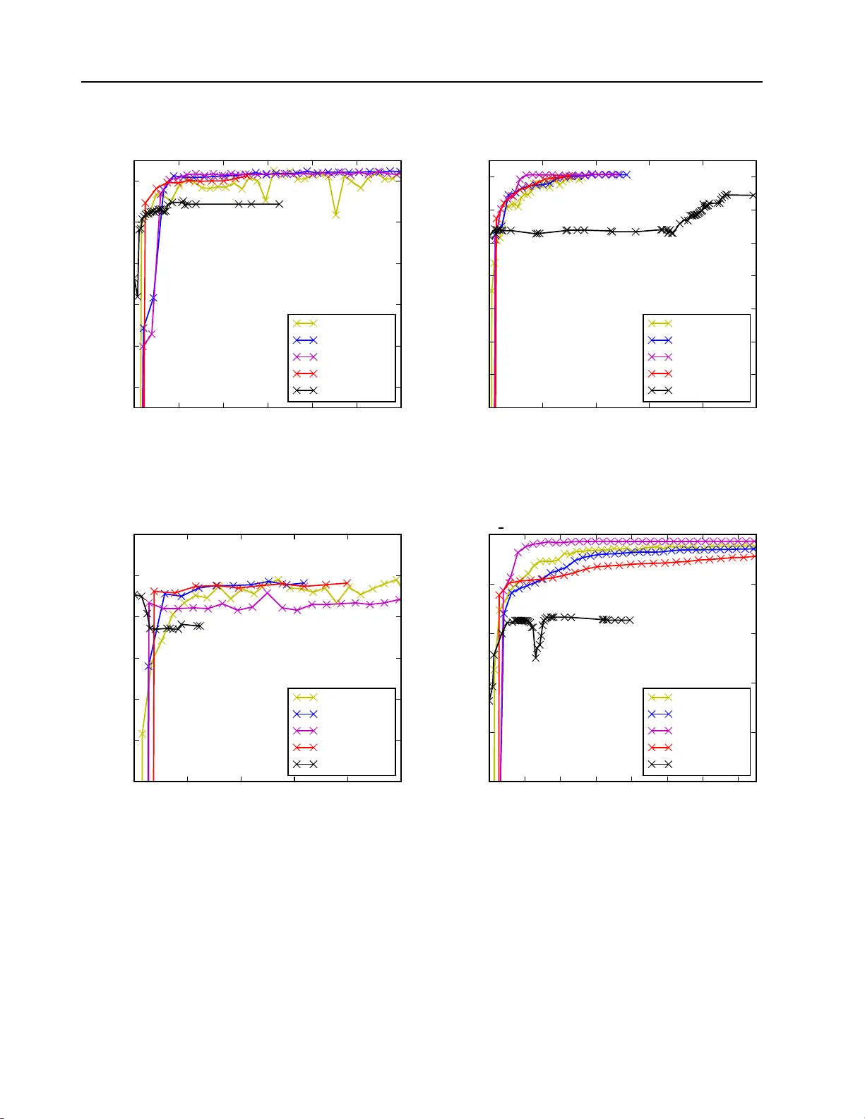
F aster v ariational GP-classification 1 F aster va riational indu cing input Gauss ian p ro cess classification P. Izmailov 1 , D. Kr op otov 1 , izmailovpav el@gmail.c om, dmitry.krop otov@gmail .com 1 Lomonoso v Mosco w State Univ ersity , 1 L eninskie G ory , Mosco w, Russia Bac kground : Gaussian pro cesses (GP) pro vide an elegan t a nd effectiv e app r oac h t o learning in k ernel mac hines. This approac h leads to a highly in terpretable mo del and allo ws using the ba yesian framew ork for model adaptation and incorp orating the prior kno wledge ab out the problem. GP framew ork is successfully applied t o regression, cla ssification a nd dimensionalit y reduction problems. Unfortunately , th e standard metho ds for b oth GP-regression and GP- classification scale a s O ( n 3 ), where n is the size of the d ataset, whic h mak es them inapplicable to big data problems. A v ariet y of metho ds hav e b een prop osed to ov ercome this limitation b oth for reg ression and cla ssification problems. The most successful rece n t metho d s are b ased on the concept of inducing in puts. Th ese metho d s reduce the computational complexit y to O ( nm 2 ), w here m is the num b er of inducing inputs with m typica lly m uch less, than n . In this w ork we fo cu s on classifica tion. The cur ren t state-of-the-art metho d for this p roblem is based on sto c hastic optimization of an evidence lo wer b ound , th at dep ends on O ( m 2 ) parameters. F or complex pr oblems, the required num b er of ind ucing p oints m is fairly b ig, making th e optimization in this metho d challe nging. Metho ds : W e analyze the structure of v ariational lo wer b ound that app ears in inducing input GP classification. First w e notice th at usin g quadratic appro ximation of sev eral terms in this b ound, it is p ossible to obtain analytical expr essions for optimal v alues of most of the optimizatio n parameters, th us sufficien tly redu cing the dimension of optimization space. Then w e pro vide t wo metho ds for constructing necessary quadr atic app ro ximations. One is based on Jaakko la-Jordan b ound for logistic function and the other one is derived using T a ylor expansion. Results : W e prop ose tw o new v ariational lo we r b ounds for inducing input GP classificatio n that dep end on a num b er of parameters. Then w e prop ose sev eral metho ds for optimizat ion of these b ounds and compare the r esulting algorithms with the stat e-of-the-art approac h based on sto c hastic optimization. Exp erimen ts on a bun c h of classification d atasets sho w that the new metho ds p erform as wel l or b etter than the existing one. How ev er, n ew metho ds don’t require an y tunable parameters and can w ork in settings within a big range of n and m v alues th u s sig nifican tly simplifying trainin g of GP classification mo d els. Keyw ords : Gaussian pr o c ess; classific ation; variational infer enc e; big dat a; inducing inputs; optimization ; variatio nal lower b ound 1 Intro duction Gaussian pro cesses (GP) provide a prior o v er functions and allo w finding complex regularities in data. G a ussian pro cesses are successfully used for classification/regression problems and dimensionalit y reduction [5]. In this work w e consider the classific ation problem only . Standard metho ds for GP-classification scale as O ( n 3 ), where n is the size of a training dataset. This complexit y mak es them inapplicable to big data problems. Therefore, a v ariety of metho ds w ere in tro duced to o v ercome this limitations [8 – 10]. In the pap er w e fo cus on metho ds based on so called inducing inputs. The pap er [6] in tro duces the inducing inputs approac h for training GP mo dels for regression. This approac h is based on v ariatio nal inference and propo ses a part icular low er b o und for mar g inal lik eliho o d (evidenc e). This b ound is then maximized w.r.t. parameters of kerne l function of the Gauss ian pro cess, th us fitting the model P . Izmailov 1 , D. Krop otov 1 , 2 to data. The computational complexit y of this metho d is O ( nm 2 ), where m is the n umber of inducing inputs used by the mo del and is assumed to b e substan tially smaller than n . The pap er [1] dev elops these ideas by show ing how to apply sto c hastic optimization to the e vidence lo w er b ound similar to the o ne used in [6]. Ho w ev er, a new lo wer b ound dep ends on O ( m 2 ) v ar iational parameters that mak es optimization in the case of big m c hallenging. The pap er [2] sho ws ho w to apply the a ppro ac h from [1] to the GP-classification problem. It pro vides a low er b ound that can b e optimized w.r.t. k ernel para meters and v ariationa l pa- rameters us ing stochastic optimization. Ho w ev er, the lo w er bound deriv ed in [2] is in tractable and has to b e approximated via Gauss-Hermite quadrat ures or other in tegral approximation tec hniques. This lo wer b ound is also fit for sto chastic optimization a nd dep ends o n O ( m 2 ) parameters. In this work w e dev elop a new approac h for training induc ing input GP mo dels fo r classifica- tion problem s. Here we ana lyze a structure o f v ar ia tional lo w er b ound from [2]. W e notice that using quadratic appro ximation of sev eral terms in this b ounds it is p ossible to obtain analytical expressions for optimal v alues of the most of optimization parameters th us sufficien tly reducing the dimension of optimizatio n space. So, we provide tw o metho ds fo r constructing necessary quadratic approx imations — one is based on Jaakk ola-Jordan b o und for logistic function, and the other one is de riv ed using T a ylor expansion. The pap er is org anized as follo ws. In section 2 w e describe the standard GP-classification framew ork and its main limitations. In sec tion 3 w e in t r o duce the concept of inducing inputs and deriv e the evidence low er b ound of [2]. Section 4 consists of our main contribution - t w o new tractable evidence lo we r b ounds and differen t metho ds for their optimizatio n. Section 5 pro vides exp erimen t al comparison of our new m etho ds w ith the existing approach from [2 ] and the last section concludes the paper. 2 GP-classification mo del In this section w e review classic Gaussian Pro cesses (GP) framew ork and its application for classification problems (see [5] for detailed discussion). 2.1 Gaussian pro cess definition A G aussian pro cess is a collection of rando m v ariables, an y finite num b er of which hav e a joint Gaussian distribution. W e will only consider pro cesses, that tak e place in a finite-dimensional real space R d . In this case, f is a Gaussian pro cess, if for any k , for an y t 1 , . . . , t k ∈ R d the join t distribution ( f ( t 1 ) , . . . , f ( t k )) T ∼ N ( m t , K t ) for some m t ∈ R k and K t ∈ R k × k . The mean m t of this distribution is defined by the mean function m : R d → R of the Gaussian pro cess: m t = ( m ( t 1 ) , . . . , m ( t k )) T . Similarly , the cov ariance matrix K t is defined b y the co v ariance function k : R d × R d → R : K t =     k ( t 1 , t 1 ) k ( t 1 , t 2 ) . . . k ( t 1 , t n ) k ( t 2 , t 1 ) k ( t 2 , t 2 ) . . . k ( t 2 , t n ) . . . . . . . . . . . . k ( t n , t 1 ) k ( t n , t 2 ) . . . k ( t n , t n )     . (1) F aster v ariational GP-classification 3 0 . 0 0 . 2 0 . 4 0 . 6 0 . 8 1 . 0 − 1 . 2 − 1 . 0 − 0 . 8 − 0 . 6 − 0 . 4 − 0 . 2 0 . 0 0 . 2 1-dimensional Gaussian pro cess Figure 1 On e-dimensional Gaussian pro cesses It’s straightforw ard then, that a Gaussian pro cess is completely defined b y its mean and co v ariance functions. W e will use t he follo wing notat io n: f ∼ G P ( m ( · ) , k ( · , · )) While the mean function m can b e an arbit r a ry real-v a lued function, the co v ariance f unction k has to b e a k ernel, so that the cov ariance matrices (1) it implies are symmetric and p ositiv e definite. Fig. 1 s ho ws an example of a one-dimensional Gaussian pro cess. The dark blue line is the mean function of the pro cess, the light blue region is the 3 σ -region, and differen t color curv es are samples from the pro cess. 2.2 Gaussian pro cess classification No w we apply Gaussian pro cesses to a binary classific ation problem. Suppose, w e hav e a dataset { ( x i , y i ) | i = 1 , . . . , n } , where x i ∈ R d , y i ∈ {− 1 , 1 } . Denote the matrix comprised of p oin ts x 1 , . . . , x n b y X ∈ R n × d and the vec tor o f corresp onding class labels y 1 , . . . , y n b y y ∈ {− 1 , 1 } n . The task is to predict the class lab el y ∗ ∈ {− 1 , 1 } at a new p oin t x ∗ ∈ R d . W e conside r the follo wing mo del. First w e in tro duce a la ten t function f : R d → R and put a zero-mean GP prior ov er it : f ∼ G P (0 , k ( · , · )) for some co v ariance function k ( · , · ). F or no w the co v ariance function is supp osed to b e fixed. Then we consider t he probability of the ob ject x ∗ b elonging to p ositive class to b e equal to σ ( f ( x ∗ )) for the c hosen sigmoid function σ : p ( y ∗ = +1 | x ∗ ) = σ ( f ( x ∗ )) . (2) In this w ork w e use the log istic function σ ( z ) = (1 + exp( − z ) ) − 1 , how eve r one could use other sigmoid functions a s w ell. The probabilistic mo del for this setting is giv en b y p ( y , f | X ) = p ( y | f ) p ( f | X ) = p ( f | X ) n Y i =1 p ( y i | f i ) , (3) P . Izmailov 1 , D. Krop otov 1 , 4 f 1 f 2 f n . . . y 1 y 2 y n . . . Figure 2 GP-classification graphical mo del where p ( y i | f i ) is sigmoid lik eliho o d (2) a nd p ( f | X ) = N ( f | 0 , K ( X , X )) is GP prio r. The corresp onding probabilistic graphical mo del is giv en in fig. 2 . No w inference in the model (3) can b e done in t w o steps. First, for new data point x ∗ w e should find the conditional distribution o f the corresponding v alue of the laten t pro cess f ∗ . This can b e done as f o llo ws p ( f ∗ | y , X , x ∗ ) = Z p ( f ∗ | f , X , x ∗ ) p ( f | y , X ) d f . (4) Second, the probability that x ∗ b elongs to the p ositiv e class is obtained by mar ginalizing ov er the laten t v ariable f ∗ . p ( y ∗ = +1 | y , X , x ∗ ) = Z σ ( f ∗ ) p ( f ∗ | y , X , x ∗ ) d f ∗ . (5) Unfortunately , b oth in tegrals (4) and (5) are intractable since they inv o lv e a pro duct of sigmoid functions and normal distributions. Th us, w e ha v e to use some in tegra l-approx imation tec hniques to estimate the pre dictiv e distribution. F o r example, one can use L a place approx imation metho d, whic h builds a Gaussian approx - imation q ( f | y , X ) to the true p osterior p ( f | y , X ). Substituting this Gaussian approximation bac k into (4) w e obtain a tractable in tegral. The predictiv e distribution (5) remains in tractable, but since this is a o ne- dimensional in tegra l it can b e easily estimated by quadratures or o ther tec hniques. The mo r e detailed deriv ation of this algorithm and another algorithm, based on Exp ectatio n Propag ation, can b e found in [5]. Computational complexit y of computing the predictiv e distribution b oth for the Laplace appro ximation metho d and Exp ectation propagation scales as O ( n 3 ) since they b oth require to in vert n × n matrix K ( X , X ). In section 3 w e describ e the concept of inducing p oints aimed to reduce this complexit y . 2.3 Mo del adaptation In the previous section w e described ho w to fit a G a ussian pro cess to the data in the clas sification problem. Ho we v er, we only considered G aussian pro cesses with fixed co v ariance functions. This mo del can b e rather limiting. Most of the p opular co v aria nce functions hav e a set of parameters, whic h w e refer t o as co v ariance (or k ernel) hyper-para meters. F or example, the squared exp onen tial co v ariance func- tion k S E ( x , x ′ ; θ ) = σ 2 exp  − k x − x ′ k 2 l 2  F aster v ariational GP-classification 5 has t w o par a meters θ – v ariance σ and length-scale l . An example o f a mor e complicated p opular co v a r ia nce function is the Matern function, g iv en b y k M atern ( x , x ′ ; θ ) = 2 1 − ν Γ( ν ) √ 2 ν k x − x ′ k l ! ν K ν √ 2 ν k x − x ′ k l ! , with t w o p ositiv e parameters θ = ( ν, l ). Here K ν is a mo dified Bessel function. In order to get a go o d mo del for the data, one should find a go o d set of k ernel h yp er- parameters θ . Bay esian paradigm prov ides a w a y o f tuning the k ernel hyper-para meters o f the GP-mo del thr o ugh ma ximization of the mo del evidence (marginal like liho o d), that is give n b y p ( y | X , θ ) = Z p ( y | f ) p ( f | X , θ ) d f → max θ . (6) Ho wev er, t his in tegral is intractable for the mo del (3) since it in volv es a pro duct of sig- moid f unctions and no rmal distribution. In subsequen t sections w e describ e sev eral meth- o ds to construct a v aria t io nal low er b ound to the marginal lik eliho o d. Maximizing t his lo w er b ound with resp ect to kernel h yp er- parameters θ , one could fit the mo del to the data. 3 V a riational inducing p oint GP-cl assification In the previous section w e sho w ed how Gaussian pro cesses can b e applied to solv e classification problems. The computational complexit y o f G P for classification scales as O ( n 3 ), that mak es this metho d inapplicable to big da t a problems. A num b er of appro ximate metho ds hav e b een prop osed in the literature for b oth GP- regression and GP-classification [8 – 10]. In this pa p er we consider metho ds based on the concept of inducing inputs. These metho ds construct an approx imation based on the v alues of the pro cess at some m < n p o ints. These p oin ts are referred to as inducing p oints . The idea is the following. The hidden G a ussian pro cess f corresp onds to some smo oth lo w-dimensional surface in R d . This surface can in fact b e w ell approximated b y another Ga ussian pro cess with prop erly c hosen m training p oin ts Z = ( z 1 , . . . , z m ) T ∈ R m × d and pro cess v alues at that p oints u = ( u 1 , . . . , u m ) T (inducing inputs). Then predictions o f this new pro cess at training p o ints are used for constructing appro ximate p osterior distribution for p ( f | y , X ). The p ositions Z of inducing inputs can b e learned within training pro cedure. How ev er, for simplicit y in the follo wing w e clusterize the dataset X in to m clusters using K- means and choose Z to b e cluster cen tr es. In practice w e observ e that this approac h w o rks w ell in a lmo st all the cases. 3.1 Evidence low er b ound In the follo wing w e use a v ariational approac h for solving maxim um evidence problem (6). In this approac h an evidence lo w er b ound is introduced, that is simpler to compute than the evidence itself. Then t his low er b ound is maximized w.r.t. k ernel h yp erpara meters θ and additional v ar iational parameters used fo r constructing the low er b ound. Let’s consider the following a ug men ted probabilistic mo del: p ( y , f , u | X , Z ) = p ( y | f ) p ( f , u | X , Z ) = n Y i =1 p ( y i | f i ) p ( f , u | X , Z ) . (7) The graphical mo del for the mo del (7) is sho wn in fig. 3. Note that margina lizing the mo del (7) w.r.t u giv es the initial mo del (3). P . Izmailov 1 , D. Krop otov 1 , 6 f 1 f 2 f n . . . y 1 y 2 y n . . . u Figure 3 GP-classification graphical mo del W e denote the cov ariance matrix comprised of pairwise v alues of the co v ar ia nce function k ( · , · ) o n the p o in ts Z by K ( Z , Z ) = K mm ∈ R m × m . Similarly , w e define K nn = K ( X , X ) ∈ R n × n and K nm = K ( X , Z ) = K T mn ∈ R n × m . As u and f are generated from the same Gaussian pro cess with zero-mean prior, p ( f , u | X , Z ) = N ([ f , u ] | [ 0 , 0 ] , K ([ X , Z ] , [ X , Z ])) , p ( u | Z ) = N ( u | 0 , K mm ) , p ( f | u , X , Z ) = N ( f | K nm K − 1 mm u , ˜ K ) , (8) where ˜ K = K nn − K nm K − 1 mm K mn . In the follo wing for simplicit y w e omit dep endence on X and Z in a ll fo rm ulas. Note that w e do not consider optimization w.r.t. the se v alues. Applying the standard v ariationa l low er b o und (see, for example [3]) to the augmen ted mo del (7), we obta in the follo wing inequalit y: log p ( y ) > E q ( u , f ) log p ( y , u , f ) q ( u , f ) = E q ( u , f ) log p ( y | f ) − KL ( q ( u , f ) k p ( u , f )) for an y distribution q ( u , f ). This inequalit y b ecomes equality for the true po sterior distribution q ( u , f ) = p ( u , f | y ). Next we restrict the v ariatio nal distribution q ( u , f ) to b e of the form q ( u , f ) = p ( f | u ) q ( u ) , (9) where q ( u ) = N ( u | µ , Σ ) for some µ ∈ R m , Σ ∈ R m × m and p ( f | u ) is determined b y (8). This is the k ey approximation step in inducing p oin ts approach fo r Gaussian pro cesses. The c hosen family (9) subsumes that with large enough m a ll information ab out t he hidden pro cess v alues f at training p oin ts can b e successfully r estored from the v alues u at inducing inputs, i.e. p ( f | u , y ) ≈ p ( f | u ). The form (9) of the v aria t ional distribution implies a Gaussian marginal distribution q ( f ) = Z p ( f | u ) q ( u ) d u = N ( f | K nm K − 1 mm µ , K nn + K nm K − 1 mm ( Σ − K mm ) K − 1 mm K mn ) . F aster v ariational GP-classification 7 As log p ( y | f ) dep ends on u only thro ugh f , the exp ectation E q ( u , f ) log p ( y | f ) = E q ( f ) log p ( y | f ) = n X i =1 E q ( f i ) log p ( y i | f i ) , where q ( f i ) is the marginal dis tribution of q ( f ): q ( f i ) = N ( f i | k T i K − 1 mm µ , K ii + k T i K − 1 mm ( Σ − K mm ) K − 1 mm k i ) = N ( f i | m i , S 2 i ) , (10) and k i is the i -th column o f matrix K mn . Finally , KL ( q ( u , f ) k p ( u , f )) = KL ( q ( u ) p ( f | u ) k p ( u ) p ( f | u )) = KL ( q ( u ) k p ( u )) . Com bining ev erything back to gether, w e obtain the e vidence low er b o und log p ( y ) > n X i =1 E q ( f i ) log p ( y i | f i ) − KL ( q ( u ) k p ( u )) . (11) Note that the KL- div ergence term in the low er b ound (1 1) can b e computed analytically since it is a KL-div ergence b etw een tw o normal distributions. In o rder to compute the exp ec- tations E q ( f i ) log p ( y i | f i ), we hav e t o use in tegral a pproximating tec hniques. The evidence lo w er b ound (ELBO) ( 1 1) can b e maximized with resp ect to v ariational param- eters µ , Σ and k ernel h yp er-parameters. Using the optimal distribution q ( u ), w e can p erform predictions for new data p oint x ∗ as follow s p ( f ∗ | y ) = Z p ( f ∗ | u , f ) p ( u , f | y ) d u d f ≈ Z p ( f ∗ | u , f ) q ( u , f ) d u d f = = Z p ( f ∗ | u , f ) p ( f | u ) q ( u ) d u d f = Z p ( f ∗ | u ) q ( u ) d u . The la st in tegral is tractable since both terms p ( f ∗ | u ) and q ( u ) are normal distributions. Note, that in case of regression with Ga ussian noise the distributions p ( y i | f i ) are G a ussians and th us the exp ectations E q ( f i ) log p ( y i | f i ) are tra ctable. Paper [1] suggests ma ximization of the low er b ound (11) with respect to µ , Σ and co v aria nce h yp er-pa r ameters with sto c hastic optimization tec hniques for GP-r egression. 3.2 SVI metho d In case of classification w e can’t analytically compute the exp ectations E q ( f i ) log p ( y i | f i ) in the low er b ound (11). Ho w ev er, the exp ectations are o ne- dimensional G a ussian integrals and can thus b e effectiv ely approximated with a range of tec hniques. In pap er [2] Gauss-Hermite quadratures are used f or this purp ose. Note that the lo w er b ound (11) has the form ” sum ov er training ob jects”. Hence this b o und can b e maximized using sto c hastic optimizatio n tec hniques. P ap er [2] suggests to maximize the low er b o und (11) with respect to the v ariatio na l parameters µ , Σ and k ernel h yp er-parameters θ using sto c hastic optimization. W e refer to t his me tho d as svi metho d (abbreviation for Sto c hastic V aria tional Inference). The low er b ound (11) and all it’s deriv ativ es can b e computed in O ( nm 2 + m 3 ). This complexit y ha s a linear dep endence on n , hence svi metho d can b e applied for the case of big training da ta. P . Izmailov 1 , D. Krop otov 1 , 8 4 T ractable evidence lo w er b ound fo r GP-classification In the previous section we describ ed the sv i metho d. It is based on sto chastic o ptimization of the lo w er b ound (11) for marginal lik eliho o d and the lo wer b ound itself is computed in O ( nm 2 ). But the bo und dep ends on O ( m 2 ) par ameters whic h make s the optimization problem hard to solv e whe n a big num b er of inducing p oin t s is needed. F o r GP-regression the situation is similar. Paper [1] describ es a metho d analogical t o the svi metho d for classification. The only difference is that the low er b ound b ecomes tractable in case of regression. Then the pap er [6] tries to solv e the problem o f big O ( m 2 ) nu m b er of par ameters in the algorithm from [1] in the follo wing w ay . In case of regression the lo wer b o und (11) can b e analytically optimise d with r esp ect to v ariatio na l par a meters µ , Σ . Doing so and substituting the optimal v alues bac k in to the low er b ound, one can obta in a new low er b ound to the margina l lik eliho o d that dep ends solely on kerne l hyper-parameters θ . This simplifies the optimization problem b y dra matically reducing the num b er of optimization parameters . Unfortunately , this new b ound doesn’t hav e a for m of ”sum o v er ob jects”, hen ce sto chastic optimization metho ds are no longer a pplicable here. How ev er, in our exp erimen ts we’v e found that ev en for fa irly big datasets the metho d f r om [6] outp erfo r ms [1] despite the lac k of sto c hastic optimization. In the follow ing subsection w e devise an approach similar to the metho d of [6] f or the case o f classification. W e pro vide a tractable ev idence lo we r bo und and analytically maximiz e it with resp ect to v ariational parameters µ and Σ . Substituting t he optimal v alues of these parameters bac k in to the lo w er b ound w e obta in a new low er b o und, that dep ends only on k ernel h yp er-parameters θ . 4.1 Global evidence lo wer b ound In order to deriv e a tractable lo w er b ound for ( 1 1), we seek a quadratic approximation to the lo g-logistic function log p ( y i | f i ) = log σ ( y i f i ), where log σ ( t ) = − log ( 1 + exp( − t )). The pap er [4] provides a global parametric quadratic lo w er b ound for this function: log σ ( t ) > t 2 − ξ t 2 + lo g σ ( ξ t ) − λ ( ξ t )( t 2 − ξ 2 t ) , ∀ t where λ ( ξ t ) = tanh( ξ t ) / (4 ξ t ) and ξ t ∈ R is a parameter of the b ound. This b ound is tight when t 2 = ξ 2 t . Substituting this b ound bac k to (11) with separate v alues ξ = { ξ i | i = 1 , . . . , n } for ev ery data p oint, w e obtain a tra cta ble lo w er b ound log p ( y ) > n X i =1 E q ( f i ) log p ( y i | f i ) − KL ( q ( u ) k p ( u )) = n X i =1 E q ( f i ) log σ ( y i f i ) − KL ( q ( u ) k p ( u )) > > n X i =1  E q ( f i )  log σ ( ξ i ) + y i f i − ξ i 2 − λ ( ξ i )( f 2 i − ξ 2 i )  − KL ( q ( u ) k p ( u )) = = n X i =1  log σ ( ξ i ) − ξ i 2 + λ ( ξ i ) ξ 2 i  + 1 2 µ T K − 1 mm K mn y − tr  Λ ( ξ )( K nn + K nm K − 1 mm ( Σ − K mm ) K − 1 mm K mn )  − − µ T K − 1 mm K mn Λ ( ξ ) K nm K − 1 mm µ − KL ( q ( u ) k p ( u )) = J ( µ , Σ , ξ , θ ) , where Λ ( ξ ) =     λ ( ξ 1 ) 0 . . . 0 0 λ ( ξ 2 ) . . . 0 . . . . . . . . . . . . 0 0 . . . λ ( ξ n )     . F aster v ariational GP-classification 9 Algorithm 1 vi-JJ metho d Input: n upd , n f un Output: θ , µ , Σ µ , Σ ← 0 , I rep eat ˜ µ , ˜ Σ ← µ , Σ for j ← 1 , . . . , n upd : // stage 1: up dating µ , Σ , ξ m t , S t ← k T t K − 1 mm ˜ µ , K tt + k T t K − 1 mm ( ˜ Σ − K mm ) K − 1 mm k t , t = 1 , . . . , n ˜ ξ t 2 ← m 2 t + S 2 t , t = 1 , . . . , n ˜ µ , ˜ Σ ← ˆ µ ( ˜ ξ ), ˆ Σ ( ˜ ξ ) // see (12), (13 ). µ , Σ , ξ ← ˜ µ , ˜ Σ , ˜ ξ θ = minimize( ˆ J ( · , ξ ), metho d=’L-BF GS-B’, maxfun= n f un ) // stage 2: up dating θ un til con v ergence Differen tia ting J with r esp ect to µ and Σ and setting the de riv at iv es to zero, we obtain ˆ Σ ( ξ ) = (2 K − 1 mm K mn Λ ( ξ ) K nm K − 1 mm + K − 1 mm ) − 1 , (12) ˆ µ ( ξ ) = 1 2 ˆ Σ ( ξ ) K − 1 mm K mn y . (13) Substituting the optimal v alues of v ariationa l parameters bac k to the low er b ound J and omitting the terms not dep ending on θ and ξ , w e obtain a c ompact low er b ound ˆ J ( θ , ξ ) = n X i =1  log σ ( ξ i ) − ξ i 2 + λ ( ξ i ) ξ 2 i  + 1 8 y T K nm B − 1 K mn y + 1 2 log | K mm | − 1 2 log | B | − tr( Λ ( ξ ) ˜ K ) , (14) where ˜ K = K nn − K nm K − 1 mm K mn , B = 2 K mn Λ ( ξ ) K nm + K mm . In the follow ing we consider three differen t metho ds fo r maximizing the low er b ound ˆ J ( θ , ξ ). Note, that give n t he v alues o f µ , Σ , θ , we can maximize J ( µ , Σ , ξ , θ ) with respect to ξ analytically . The optimal v alues for ξ are giv en b y ξ 2 i = E q ( f ) f 2 i = m 2 i + S 2 i . (15) The v alues m i and S i w ere defined in ( 1 0). In o ur first metho d w e us e analytical formulas (15) to recompute the v alues of ξ and use gradient-based o ptimizatio n to maximize the b o und with resp ect to θ . The pseudo co de is given in Alg. 1. W e will refer to t his method as vi-JJ , where JJ stands fo r Jaakk ola and Jordan, the a uthors o f [4]. Note that the computational complexit y of one iteration of this metho d is O ( nm 2 ), t he s ame as f or the svi metho d. Our second metho d uses gra dien t-ba sed optimization to maximize ˆ J with resp ect to b oth θ and ξ . Note that in this metho d w e don’t hav e to rec ompute µ and Σ at eac h iteration whic h mak es the metho ds itera t ions empirically faster for big v alues of m . W e refer to this metho d as vi-JJ-full . P . Izmailov 1 , D. Krop otov 1 , 10 Finally , vi-JJ-hybrid is a com bination of the t w o metho ds describ ed ab ov e. The general sc heme of this metho d is the same as vi-JJ . In the vi-JJ-hybri d metho d w e use analytical form ulas to recompute ξ as w e do in the vi-JJ metho d at stage 1, but at stage 2 w e use gradien t - based optimization with resp ect to b oth ξ and θ . The virtues of t his metho d will b e described in the ex p erimen ts section. 4.2 T ractable lo cal approxi mation to the evidence low er b ound Another w a y to obtain a tractable a pproximation to the lo wer b ound (1 1) is to use a lo cal quadratic appro ximation fo r the log- logistic function log p ( y i | f i ). In this w ay w e p erform a second-order T aylor expansion of this f unction at p oints ξ = { ξ i | i = 1 , . . . , n } : log p ( y i | f i ) ≈ − log(1 + exp( − y i ξ i )) + y i 1 + exp( y i ξ i ) ( f i − ξ i ) − y 2 i exp( y i ξ i ) 2(1 + exp( y i ξ i )) 2 ( f i − ξ i ) 2 . (16) The follo wing deriv ation is analogical to t he deriv ation in the previous section. Substituting the approx imation (16) into the low er bound (11), w e obtain log p ( y ) > n X i =1 E q ( f i ) log p ( y i | f i ) − KL ( q ( u ) k p ( u )) ≈ ≈ − n X i =1 log(1 + exp( − y i ξ i )) + ϕ ( ξ ) T ( K nm K − 1 mm µ − ξ ) − − tr  Ψ ( ξ )( K nn + K nm K − 1 mm ( Σ − K mm ) K − 1 mm K mn )  − ( K nm K − 1 mm µ − ξ ) T Ψ ( ξ )( K nm K − 1 mm µ − ξ ) − − 1 2  log | K mm | | Σ | − m + tr( K − 1 mm Σ ) + µ T K − 1 mm µ  . Here Ψ ( ξ ) is a diagonal matrix Ψ ( ξ ) =     ψ ( ξ 1 ) 0 . . . 0 0 ψ ( ξ 2 ) . . . 0 . . . . . . . . . . . . 0 0 . . . ψ ( ξ n )     , where ψ ( ξ i ) = y 2 i exp( y i ξ i ) 2(1 + exp( y i ξ i )) 2 . Differen tia ting the approx imate b ound with resp ect to µ , Σ , and ξ , and setting the deriv a- tiv es to zero, w e obtain the f ollo wing form ulas for optimal v alues of these parameters: ˆ Σ ( ξ ) =  2 K − 1 mm K mn Ψ ( ξ ) K nm K − 1 mm + K − 1 mm  − 1 , (17) ˆ µ ( ξ ) = ˆ Σ ( ξ ) K − 1 mm K mn v ( ξ ) , (18) ξ i = m i . Here v ( ξ ) = ϕ ( ξ ) + 2 Ψ ( ξ ) ξ , F aster v ariational GP-classification 11 0 . 0 0 . 2 0 . 4 0 . 6 0 . 8 1 . 0 1 . 2 1 . 4 Time (seco nds) 0 . 65 0 . 66 0 . 67 0 . 68 0 . 69 0 . 70 0 . 71 0 . 72 0 . 73 0 . 74 Validation Accuracy german dataset, n = 800, d = 24 , m = 2 0 svi-AdaDelta vi-JJ vi-T aylor vi-JJ-hybrid vi-JJ-full 0 . 0 0 . 2 0 . 4 0 . 6 0 . 8 1 . 0 Time (seco nds) 0 . 92 0 . 93 0 . 94 0 . 95 0 . 96 0 . 97 0 . 98 Validation Accuracy svmguide dataset, n = 3089, d = 4, m = 25 svi-AdaDelta vi-JJ vi-T aylor vi-JJ-hybrid vi-JJ-full Figure 4 Metho ds p erformance on small datasets and ϕ ( ξ ) is a vec tor, composed of ϕ ( ξ ) i = y i 1 + exp( y i ξ i ) . Substituting the optimal v alues for µ and Σ , giv en b y (17), (18), bac k in to the a pproximate b ound, and omiting the t erms, that do not dep end on θ , w e obtain the f o llo wing approximate lo w er bound: ˜ J ξ = 1 2 v ( ξ ) T K nm B − 1 K mn v ( ξ ) + 1 2 log | K mm | − 1 2 log | B | − tr( Ψ ( ξ ) ˜ K ) , (19) where B = 2 K mn Ψ ( ξ ) K nm + K mm . Note that the lo w er b o und (19 ) is not a global low er b o und for the log-evidence lo g p ( y ). Ho wev er, lo cally we get a go o d approximation of the ev idence low er b ound (11). F o r ma ximizing the approximate lo w er b ound ( 1 9) w e consider a metho d, analogical to vi-JJ . In order to sp ecify this metho d we simply substitute the b o und ˆ J ( · , ξ ) b y ˜ J ξ in the second stage in Alg. 1. W e will refer to this metho d as vi-Tay lor . The computational c omplexit y of one iteration of this me tho d is once again O ( nm 2 ). 5 Exp eriments In this section we empirically compare the deriv ed vi-JJ , vi-Taylor , vi-JJ-full and vi-JJ-hybri d metho ds with svi . Belo w w e describe the setting of the exp eriments and discu ss their results. 5.1 Exp erimen tal setting In our exp erimen ts w e compared 5 me tho ds for v ariationa l inducing po in t GP-classification: – svi-AdaDelta uses the AdaDelta o ptimizatio n metho d for maximization of the low er b o und (11) as it is done in the pap er [2]; P . Izmailov 1 , D. Krop otov 1 , 12 – vi-JJ w as describ ed in section 4 . 1; – vi-Taylor w as describ ed in section 4 . 2; – vi-JJ-full w as describ ed in section 4 . 1 ; – vi-JJ-hybrid w as describ ed in section 4 . 1. W e also tr ied using deterministic L-BFGS-B optimization metho d for maximizing the evidence lo w er b o und (1 1), but it w ork ed subs tan tia lly w orse than all the o ther metho ds. Note, tha t a ll the metho ds ha v e the same complexit y of ep o c hs O ( nm 2 ). T able 1 show s whic h v ariables are optimized nu merically and which are optimized ana lytically f or eac h method. In our exp erimen ts we didn’t optimize the lo w er b ound with resp ect to the p ositions Z of inducing p o in ts. Instead we used K -means clustering pro cedure with K equal to the num b er m o f inducing inputs and to ok clusters cen tres as Z . Also we used the squared exp onen tial co v ariance function (se e section 1) in all exp erimen ts with a Ga ussian no ise term. The sto c hastic metho d svi-AdaDelta requires the user to man ually sp ecify the learning rate and t he batc h size f or the optimization metho d. F or the fo rmer w e had to run the metho d with differen t learning rates a nd c ho ose the v alue that resulted in the f a stest conv ergence. W e used the learning r ates from a fixed grid with a step of 0 . 1. It alw a ys happ ened, tha t for the largest v alue from t he g rid the metho d div erged, and for the smallest the metho d con verged slo we r, than for s ome medium v alue, v erifying, that the optimal learning rate w as somewhe re in the range. T o c ho ose the batc h size w e used the following conv ention. F or small german and svmguide dat asets we’v e set the batc h size to 5 0 . F or other datasets w e used approximately n 100 as the batch size, where n is the s ize of the tra ining set. F o r the vi-JJ , vi-Taylor a nd vi-JJ-hy brid in all of the experiments on ev ery iteration w e recomputed the v alues of ξ , µ , and Σ 3 times ( n upd = 3 in algorithm 1). T o tune θ , on ev ery iterat io n w e’v e r un L-BFGS-B optimizatio n metho d constrained to do no more than 5 ev aluatio ns of the low er b ound and it’s gradien t. W e found that these v alues of parameters w ork w ell for all the datasets we exp erimen ted w ith. F o r the svi-AdaDelta metho d w e used optimization w.r.t. Cholesky factor of the matr ix Σ in or der to maintain it’s p ositive definiteness, as describ ed in [2]. W e used AdaDelta optimization metho d implemen ta tion f rom the clim in to olb ox [7] as is done in the origina l pap er. F o r ev ery dataset w e exp erimente d with a n um b er of inducing p oints to verify that the results of the metho ds are close t o o ptimal. W e ev aluate the metho ds plotting the accuracy of their predictions on the test data ag ainst time. All of the plots ha v e titles of the following format. [name of the dataset] , n = [n umber of ob jects in the tra ining set] , d = [n um b er of features] , m = [n um b er of inducing inputs] T able 1 Metho ds outline Metho d Numerically optimized v ar iables Analytically optimized v ar iables svi-AdaDelt a θ , µ ∈ R m , Σ ∈ R m × m vi-JJ , vi-Taylor θ µ ∈ R m , Σ ∈ R m × m , ξ ∈ R n vi-JJ-hybri d θ , ξ ∈ R n µ ∈ R m , Σ ∈ R m × m , ξ ∈ R n vi-JJ-full θ , ξ ∈ R n µ ∈ R m , Σ ∈ R m × m F aster v ariational GP-classification 13 0 5 10 15 20 25 30 Time (seco nds) 0 . 76 0 . 78 0 . 80 0 . 82 0 . 84 0 . 86 Validation Accuracy magic telescope dataset, n = 15215, d = 10, m = 50 svi-AdaDelta vi-JJ vi-T aylor vi-JJ-hybrid vi-JJ-full 0 50 100 150 20 0 250 Time (seco nds) 0 . 80 0 . 82 0 . 84 0 . 86 0 . 88 0 . 90 0 . 92 0 . 94 Validation Accuracy ijcnn dataset, n = 35 000, d = 22, m = 100 svi-AdaDelta vi-JJ vi-T aylor vi-JJ-hybrid vi-JJ-full Figure 5 Metho ds p erformance on medium datasets 0 200 40 0 600 800 1000 Time (seco nds) 0 . 940 0 . 945 0 . 950 0 . 955 0 . 960 0 . 965 0 . 970 Validation Accuracy co d-rna dataset, n = 59535, d = 8, m = 400 svi-AdaDelta vi-JJ vi-T aylor vi-JJ-hybrid vi-JJ-full 0 20 40 60 80 1 00 120 140 Time (seco nds) 0 . 95 0 . 96 0 . 97 0 . 98 0 . 99 1 . 00 Validation Accuracy skin no nskin dataset, n = 1 96045, d = 3, m = 20 svi-AdaDelta vi-JJ vi-T aylor vi-JJ-hybrid vi-JJ-full Figure 6 Metho ds p erformance on big datasets W e also prepro cessed all the datasets by normalizing the feat ur es setting the mean of all features to 0 and the v ariance to 1 . F or dat a sets without a v aila ble test data, we us ed 20% of the data as a test set and 80% as a train set. 5.2 Results and discussion W e compared the metho ds’ performance on sev en da t asets. Here w e discuss the results. Fig. 4 pro vides the results for german and svmguide da tasets. As w e can see, on the sm all german data set the sto c hastic svi-AdaDelta method struggles, and it tak es it longer to achiev e the optimal qualit y , than for all the ot her methods, whic h sho w similar r esults. On the svmguide P . Izmailov 1 , D. Krop otov 1 , 14 0 100 200 300 400 500 Time (seco nds) 0 . 76 0 . 78 0 . 80 0 . 82 0 . 84 0 . 86 Validation Accuracy a8a dataset, n = 18156, d = 123, m = 500 svi-AdaDelta vi-JJ vi-T aylor vi-JJ-hybrid vi-JJ-full Figure 7 Metho ds p erformance on the a8a d ataset dataset it tak es vi-JJ-full and svi-AdaDelta a little bit longer to con verge, while the other three metho ds show roughly t he s ame p erformance. The results on magic tele sc op e and ijcnn data sets are pro vided in fig. 5 . On the magic telesc op e dataset t he vi-JJ and vi-Ta ylor sho w p o or quality on the first iterations, but still manage to c on verge faster, than svi- AdaDelta . On b oth datasets the vi -JJ-hybrid metho d w orks similar to vi-JJ and vi-Taylor , but shows b etter qualit y on first iterations on the magic telesc op e data. vi-JJ-full can’t conv erge to a reasonable quality on both data sets. Fig. 6 pro vides the results on big c o d-rna a nd ski n nonskin datasets. On these dat asets the vi-JJ-full once ag ain fails to achiev e a reasonable qualit y , while the other metho ds work similarly . Finally , the results on a8a data are pro vided in fig. 7. Here we use a rather big amoun t of m = 500 inducing inputs. As w e can see, the vi-JJ-full and vi-JJ-hybrid are the fastest to ac hiev e the optimal quality . The svi-AdaDel ta metho d a lso con v erges reasonably f a st, while the vi-JJ and vi-Taylor strugg le a little bit. In general vi- JJ , vi-Taylo r and vi-JJ-hyb rid metho ds p erfo rm similar to svi-AdaDelta metho d. On the big dataset skin nonskin with only 3 features the vi-JJ-hybrid is a little bit slow er t han the sto c hastic svi-AdaDel ta , but on all the other da t a sets it is b etter. The vi-Taylor a nd vi-JJ struggle with a8a , but are otherwise comparable to vi-JJ-hybrid . The sto c hastic svi-AdaDelta metho d p erforms p o orly o n small datasets and ev en o n the big skin - nonskin data do esn’t manage to substan tially outp erform the o ther metho ds, even provided a go o d v alue of lear ning rate. Finally , vi-JJ-full w o rks w ell o n small data and on the a8a , but on a ll the other datasets it do esn’t mana ge to ac hiev e a reasonable quality . 6 Conclusion In this pa p er we presen ted a new approa c h to training v ariational inducing input Gaussian pro cess classification. W e derived tw o new tractable evidence low er b ounds and describ ed s ev- eral w ays to maximize them. The resulting metho ds vi-JJ , vi-JJ-full , vi-JJ-hybrid a nd vi-Taylor are similar to the metho d of [6] for GP-regression. F aster v ariational GP-classification 15 W e pro vided an exp erimen tal comparison of our metho ds with the curren t state-of-the-art metho d svi-AdaDelta of [2]. In our exp erimental setting, our appro a c h prov ed to b e more practical, as it con verges to the optimal qualit y as fast as the svi-AdaDe lta metho d without requiring the user to manually c ho ose the parameters of the optimization me tho d. The four describ ed vi metho ds show ed similar p erformance and it’s hard to distinguish them. Ho w ev er, note that the vi-Taylor approach is more general and can be applied to the lik eliho o d functions, that are not lo gistic. W e could also easily deriv e a metho d, similar to vi-JJ-hybri d and vi-JJ-full f or the non-logistic case, but it is out of scop e of this pap er. References [1] J. Hensman, N. F usi, and N. D. Lawrence. 2013. Gaussian p ro cesses for b ig data. Pr o ceedings of the T w en ty-N in th Con f erence on Uncertain ty in Artificial Intellig ence . P . 282–290. [2] J. Hensman, G. Matthews, Z. Ghahr amani. 2015. S calable V ariational Gaussian Pro cess Clas- sification. P r o ceedings of the Eig h teen th Internatio nal Conference on Artificial Intell igence and Statistics . [3] T. Jaakk ola. 2000. T utorial on V ariational Ap pro ximation Metho ds. Adv anced Mea n Field Meth- o ds: T h eory an d Practice . P . 129–159 . [4] T. Jaakk ola, M . Jordan. 1997. A V ariational Approac h to Ba ye sian Logistic R egression Mod els and Their Extens ions . Pro ceedings of the 1997 Conference on Ar tificial Intellig ence and Statistics . [5] C. E. Rasm ussen and C. K. I. W illiams. 2006. Gaussian Pro cesses for Mac hine Learnin g . MIT Press, Cam bridge, MA. [6] M. Titsias. 2009. V ariational learning of in ducing v ariables in sparse Gaussian p r o cesses. Pr o- ceedings of the Tw elfth In ternational W orkshop on Artificial In tellige nce and Statistics . vo l. 5, P . 567–574. [7] Climin. URL: http://g ithub.co m/BRML/c limin . [8] A. S m ola, P . Bartlett 2001. S p arse greedy Gaussian p ro cess regression. Neural In formation Pr o- cessing Systems . [9] J. Qu inonero-Candela, C. Rasm u ssen 2005. A unifyin g view of sparse appro ximate Gaussian pro cess r egression. Journal of Mac hine Learning Researc h . v ol. 6, P . 1939–195 9. [10] L. Csato, M. Opp er 2002. Sp ars e online Gaussian pr o cesses. Neural Computation . vo l. 14, P . 641– 668.