Robust and Scalable Column/Row Sampling from Corrupted Big Data
Conventional sampling techniques fall short of drawing descriptive sketches of the data when the data is grossly corrupted as such corruptions break the low rank structure required for them to perform satisfactorily. In this paper, we present new sam…
Authors: Mostafa Rahmani, George Atia
1 Rob ust and Scalable Column/Ro w Sampling from Corrupted Big Data Mostafa Rahmani, Student Member , IEEE and George K. Atia, Member , IEEE Abstract —Con ventional sampling techniques fall short of drawing descriptive sk etches of the data when the data is grossly corrupted as such corruptions break the low rank structur e requir ed for them to perf orm satisfactorily . In this paper , we present new sampling algorithms which can locate the informa- tive columns in presence of severe data corruptions. In addition, we develop new scalable randomized designs of the proposed algorithms. The proposed approach is simultaneously rob ust to sparse corruption and outliers and substantially outperforms the state-of-the-art rob ust sampling algorithms as demonstrated by experiments conducted using both real and synthetic data. Index T erms —Column Sampling, Sparse Corruption, Outliers, Data Sketch, Low Rank Matrix I . I N T RO D U C T I O N Finding an informative or explanatory subset of a large number of data points is an important task of numerous machine learning and data analysis applications, including problems arising in computer vision [10], image process- ing [13], bioinformatics [2], and recommender systems [17]. The compact representation provided by the informativ e data points helps summarize the data, understand the underlying interactions, sav e memory and enable remarkable computation speedups [14]. Most existing sampling algorithms assume that the data points can be well approximated with lo w- dimensional subspaces. Howe ver , much of the contemporary data comes with remarkable corruptions, outliers and missing values, wherefore a low-dimensional subspace (or a union of them) may not well fit the data. This fact calls for robust sampling algorithms, which can identify the informative data points in presence of all such imperfections. In this paper , we present an new column sampling approach which can identify the representativ e columns when the data is grossly corrupted and fraught with outliers. A. Summary of contributions W e study the problem of informativ e column sampling in presence of sparse corruption and outliers. The ke y technical contributions of this paper are summarized next: I. W e present a ne w con vex algorithm which locates the informati ve columns in presence of sparse corruption with arbitrary magnitudes. II. W e de velop a set of randomized algorithms which pro- vide scalable implementations of the proposed method for big data applications. W e propose and implement a scalable This work was supported by NSF CAREER A ward CCF-1552497 and NSF Grant CCF-1320547. The authors are with the Department of Electrical and Computer Engi- neering, Univ ersity of Central Florida, Orlando, FL 32816 USA (e-mail: mostafa@knights.ucf.edu, george.atia@ucf.edu). column/row subspace pursuit algorithm that enables sampling in a particularly challenging scenario in which the data is highly structured. III. W e dev elop a new sampling algorithm that is robust to the simultaneous presence of sparse corruption and outlying data points. The proposed method is shown to outperform the-state-of-the-art robust (to outliers) sampling algorithms. IV . W e propose an iterativ e solver for the proposed con vex optimization problems. B. Notations and data model Giv en a matrix L , k L k denotes its spectral norm, k L k 1 its ` 1 -norm giv en by k L k 1 = P i,j L ( i, j ) , and k L k 1 , 2 its ` 1 , 2 - norm defined as k L k 1 , 2 = P i k l i k 2 , where k l i k 2 is the ` 2 - norm of the i th column of L . In an N -dimensional space, e i is the i th vector of the standard basis. For a given vector a , k a k p denotes its ` p -norm. For a given matrix A , a i and a i are defined as the i th column and i th row of A , respectiv ely . In this paper , L represents the lo w rank (LR) matrix (the clean data) with compact SVD L = UΣV T , where U ∈ R N 1 × r , Σ ∈ R r × r and V ∈ R N 2 × r and r is the rank of L . T wo linear subspaces L 1 and L 2 are independent if the dimension of their intersection L 1 ∩ L 2 is equal to zero. The incoherence condition for the row space of L with parameter µ v states that max i k e T i V k ≤ µ v r / N 2 [6]. In this paper (except for Section V), it is assumed that the giv en data follows the following data model. Data Model 1. The given data matrix D ∈ R N 1 × N 2 can be expr essed as D = L + S . Matrix S is an element-wise sparse matrix with arbitrary support. Each element of S is non-zer o with a small pr obability ρ . I I . R E L A T E D W OR K The vast majority of existing column sampling algorithms presume that the data lies in a low-dimensional subspace and look for fe w data points spanning the span of the dominant left singular v ectors [16], [34]. The column sampling methods based on the low rankness of the data can be generally categorized into randomized [7]–[9] and deterministic methods [3], [11], [13], [15], [19]. In the randomized method, the columns are sampled based on a carefully chosen probability distribution. For instance, [8] uses the ` 2 -norm of the columns, and in [9] the sampling probabilities are proportional to the norms of the rows of the top right singular vectors of the data. There are dif ferent types of deterministic sampling algorithms, including the rank re vealing QR algorithm [15], 2 and clustering-based algorithms [3]. In [11], [13], [19], [21] , sparse coding is used to le verage the self-expressiv eness property of the columns in low rank matrices to sample informativ e columns. The lo w rankness of the data is a crucial requirement for these algorithms. For instance, [9] assumes that the span of few top right singular vectors approximates the ro w space of the data, and [11] presumes that the data columns admit sparse representations in the rest of the data, i.e., can be obtained through linear combinations of few columns. Ho w- ev er , contemporary data comes with gross corruption and outliers. [21] focused on column sampling in presence of outliers. While the approach in [21] exhibits more robustness to the presence of outliers than older methods, it still ends up sampling from the outliers. In addition, it is not robust to other types of data corruption, especially element-wise sparse corruption. Element-wise sparse corruption can completely tear existing linear dependence between the columns, which is crucial for column sampling algorithms including [21] to perform satisfactorily . I I I . S H O RT C O M I N G O F R A N D O M C O L U M N S A M P L I N G As mentioned earlier, there is need for sampling algorithms capable of extracting important features and patterns in data when the data available is grossly corrupted and/or contains outliers. Existing sampling algorithms are not robust to data corruptions, hence uniform random sampling is utilized to sample from corrupted data. In this section, we discuss and study some of the shortcomings of random sampling in the context of two important machine learning problems, namely , data clustering and robust PCA. Data clustering: Informative column sampling is an effec- tiv e tool for data clustering [19]. The representative columns are used as cluster centers and the data is clustered with respect to them. Howe ver , the columns sampled through random sampling may not be suitable for data clustering. The first problem stems from the non-uniform distribution of the data points. For instance, if the population in one cluster is notably larger than the other clusters, random sampling may not ac- quire data points from the less populated clusters. The second problem is that random sampling is data independent. Hence, ev en if a data point is sampled from a given cluster through random sampling, the sampled point may not necessarily be an important descriptiv e data point from that cluster . Robust PCA: There are many important applications in which the data follows Data model 1 [5], [6], [18], [25], [26], [35], [37], [38]. In [6], it w as sho wn that the optimization problem min ˙ L , ˙ S λ k ˙ S k 1 + k ˙ L k ∗ s. t. ˙ L + ˙ S = D (1) is guaranteed to yield exact decomposition of D into its LR and sparse components if the column space (CS) and the row space (RS) of L are sufficiently incoherent with the standard basis. Howe ver , the decomposition algorithms directly solving (1) are not scalable as they need to sa ve the entire data in the working memory and have O ( r N 1 N 2 ) complexity per iteration. An ef fectiv e idea to de velop scalable decomposition algo- rithms is to e xploit the lo w dimensional structure of the LR matrix [22]–[24], [28], [30], [33]. The idea is to form a data sketch by sampling a subset of columns of D whose LR component can span the CS of L . This sketch is decomposed using (1) to learn the CS of L . Similarly , the RS of L is obtained by decomposing a subset of the ro ws. Finally , the LR matrix is reco vered using the learned CS and RS. Thus, in lieu of decomposing the full scale data, one decomposes small sketches constructed from subsets of the data columns and rows. Since existing sampling algorithms are not robust to sparse corruption, the scalable decomposition algorithms rely on uniform random sampling for column/row sampling. Howe ver , if the distributions of the columns/rows of L are highly non- uniform, random sampling cannot yield concise and descrip- tiv e sketches of the data. For instance, suppose the columns of L admit a subspace clustering structure [12], [29] as per the following assumption. Assumption 1. The matrix L can be r epresented as L = [ U 1 Q 1 ... U n Q n ] . The CS of { U i ∈ R N 1 × r/n } n i =1 ar e random r /n -dimensional subspaces in R N 1 . The RS of { Q i ∈ R r/n × n i } n i =1 ar e random r /n -dimensional subspaces in { R n i } n i =1 , r espectively , P n i =1 n i = N 2 , and min i n i r /n . The following two lemmas sho w that the sufficient number of randomly sampled columns to capture the CS can be quite large depending on the distribution of the columns of L . Lemma 1. Suppose m 1 columns ar e sampled uniformly at random with r eplacement fr om the matrix L with rank r . If m 1 ≥ 10 µ v r log 2 r δ , then the selected columns of the matrix L span the CS of L with pr obability at least 1 − δ . Lemma 2. If L follows Assumption 1, the rank of L is equal to r , r /n ≥ 18 log max i n i and n i ≥ 96 r n log n i , 1 ≤ i ≤ n , then P µ v < 1 n 0 . 5 N 2 min i n i ≤ 2 P n i =1 n − 5 i . According to Lemma 2, the RS coherency parameter µ v is linear in N 2 min i n i . The factor N 2 min i n i can be quite lar ge depending on the distribution of the columns. Thus, according to Lemma 1 and Lemma 2, we may need to sample too many columns to capture the CS if the distribution of the columns is highly non-uniform. As an example, consider L = [ L 1 L 2 ] , the rank of L = 60 and N 1 = 500 . The matrix L 1 follows Assumption 1 with r = 30 , n = 30 and { n i } 30 i =1 = 5 . The matrix L 2 follows Assumption 1 with r = 30 , n = 30 and { n i } 30 i =1 = 200 . Thus, the columns of L ∈ R 500 × 6150 lie in a union of 60 1-dimensional subspaces. Fig. 1 shows the rank of randomly sampled columns of L versus the number of sampled columns. Evidently , we need to sample more than half of the data to span the CS. As such, we cannot ev ade high- dimensionality with uniform random column/row sampling. I V . C O L U M N S A M P L I N G F R O M S PA R S E L Y C O R RU P T E D D A TA In this section, the proposed robust sampling algorithm is presented. It is assumed that the data follows Data model 1. 3 1000 2000 3000 4000 5000 6000 Number of randomly sampled columns 20 30 40 50 60 Rank of sampled columns Fig. 1. The rank of randomly sampled columns. Consider the following optimization problem min a k d i − D − i a k 0 subject to k a k 0 = r, (2) where d i is the i th column of D and D − i is equal to D with the i th column removed. If the CS of L does not contain sparse vectors, the optimal point of (2) is equiv alent to the optimal point of min a k s i − S − i a k 0 subject to l i = L − i a and k a k 0 = r , (3) where l i is the LR component of d i and L − i is the LR component of D − i ( similarly , s i and S − i are the sparse component). T o clarify , (2) samples r columns of D − i whose LR component cancels out the LR component of d i and the linear combination s i − S − i a is as sparse as possible. This idea can be extended by searching for a set of columns whose LR component can cancel out the LR component of all the columns. Thus, we modify (2) as min A k D − D A k 0 s. t. k A T k 0 , 2 = r, (4) where k A T k 0 , 2 is the number of non-zero rows of A . The constraint in (4) forces A to sample r columns. Both the objectiv e function and the constraint in (4) are non-conv ex. W e propose the following con vex relaxation min A k D − D A k 1 + γ k A T k 1 , 2 , (5) where γ is a re gularization parameter . Define A ∗ as the optimal point of (5) and define the vector p ∈ R N 2 × 1 with entries p ( i ) = k a ∗ i k 2 , where p ( i ) and a ∗ i are the i th element of p and the i th row of A ∗ , respectiv ely . The non- zero elements of p identify the representati ve columns. F or instance, suppose D ∈ R 100 × 400 follows Data model 1 with ρ = 0 . 02 . The matrix L with rank r = 12 can be expressed as L = [ L 1 L 2 L 3 L 4 ] where the ranks of { L j ∈ R 100 × 100 } 4 j =1 are equal to 5, 1, 5, and 1, respectively . Fig. 2 shows the output of the proposed method and the algorithm presented in [11]. As shown, the proposed method samples a sufficient number of columns from each cluster . Since the algorithm presented in [11] requires strong linear dependence between the columns of D , the presence of the sparse corruption matrix S seriously degrades its performance. A. Rob ust column sampling from Big data The complexity of solving (5) is O ( N 3 2 + N 1 N 2 2 ) . In this section, we present a randomized scalable approach which Fig. 2. The elements of the vector p . T e left plot corresponds to (5) and the right plot corresponds to [11]. yields a scalable implementation of the proposed method for high dimensional data reducing complexity to O ( r 3 + r 2 N 2 ) . W e further assume that the RS of L can be captured using a small random subset of the ro ws of L , an assumption that will be relax ed in Section IV -A1. The following lemma shows that the RS can be captured using few randomly sampled rows ev en if the distribution of the columns is highly non-uniform. Lemma 3. Suppose L follows Assumption 1 and m 2 r ows of L ar e sampled uniformly at random with r eplacement. If the rank of L is equal to r and m 2 ≥ 10 c r ϕ log 2 r δ , (6) then the sampled r ows span the row space of L with pr obability at least 1 − δ − 2 N − 3 1 , wher e ϕ = max( r, log N 1 ) r . The suf ficient number of sampled rows for the setup of Lemma 3 is roughly O ( r ) , and is thus independent of the distribution of the columns. Let D r denote the matrix of randomly sampled rows of D and L r its LR component. Suppose the rank of L r is equal to r . Since the RS of L r is equal to the RS of L , if a set of the columns of L r span its CS, the corresponding columns of L will span the CS of L . Accordingly , we rewrite (5) as min A k D r − D r A k 1 + γ k A T k 1 , 2 . (7) Note that we still hav e an N 2 × N 2 dimensional optimization problem and the complexity of solving (7) is roughly O ( N 3 2 + N 2 2 r ) . In this section, we propose an iterativ e randomized method which solves (7) with comple xity O ( r 3 + N 2 r 2 ) . Algorithm 1 presents the proposed solver . It starts the iteration with few randomly sampled columns of D r and refines the sampled columns in each iteration. Remark 1. In both (7) and (8), we use the same symbol A to designate the optimization variable. Howe ver , in (7) A ∈ R N 2 × N 2 , while in (8) A ∈ R m × N 2 , wher e m of or der O ( r ) is the number of columns of D s r . Here we provide a brief explanation of the different steps of Algorithm 1 : Steps 2.1 and 2.2: The matrix D s r is the sampled columns of D r . In steps 2.1 and 2.2, the redundant columns of D s r are remov ed. Steps 2.3 and 2.4: Define L s r as the LR component of D s r . Steps 2.3 and 2.4 aim at finding the columns of L r which do not lie in the CS of L s r . Define d r i as the i th column of D r . For a given i , if l r i (the LR component of d r i ) lies in the CS 4 of L s r , the i th column of F = D r − D s r A ∗ will be a sparse vector . Thus, if we remov e a small portion of the elements of the i th column of F with the largest magnitudes, the i th column of F will approach the zero vector . Thus, by removing a small portion of the elements with largest magnitudes of each column of F , step 2.3 aims to locate the columns of L r that do not lie in the CS of L s r , namely , the columns of L r corresponding to the columns of F with the largest ` 2 -norms. Therefore, in step 2.5, these columns are added to the matrix of sampled columns D s r . As an example, suppose D = [ L 1 L 2 ] + S follo ws Data model 1 where the CS of L 1 ∈ R 50 × 180 is independent of the CS of L 2 ∈ R 50 × 20 . In addition, assume D r = D and that all the columns of D s r happen to be sampled from the first 180 columns of D r , i.e., all sampled columns belong to L 1 . Thus, the LR component of the last 20 columns of D r do not lie in the CS of L s r . Fig. 3 sho ws F = D r − D s r A ∗ . One can observe that the algorithm will automatically sample the columns corresponding to L 2 because if few elements (with the largest absolute v alues) of each column are eliminated, only the last 20 columns will be non-zero. Remark 2. The appr oach pr oposed in Algorithm 1 is not limited to the pr oposed method. The same idea can be used to enable more scalable versions of e xisting algorithms. F or instance, the comple xities of [11] and [21] can be r educed fr om r oughly N 3 2 to N 2 r , which is a remarkable speedup for high dimensional data. -10 60 -5 200 0 40 150 F = D r - D r s A * 5 Rows columns 100 10 20 50 0 0 Fig. 3. Matrix F in step 2.3 of Algorithm 1. 1) Sampling fr om highly structur ed Big data: Algorithm 1 presumes that the rows of L are well distrib uted such that c 1 ˆ r randomly sampled rows of L span its RS. This may be true in many settings where the clustering structure is only along one direction (either the ro ws or columns), in which case Algorithm 1 can successfully locate the informative columns. If, howe ver , both the columns and the rows exhibit clustering structures and their distribution is highly non-uniform, neither the CS nor the RS can be captured concisely using random sampling. As such, in this section we address the scenario in which the rank of L r may not be equal to r . W e present an iterativ e CS-RS pursuit approach which conv erges to the CS and RS of L in few iterations. The table of Algorithm 2 , Fig. 4 and its caption provide the details of the proposed sampling approach along with the definitions of the used matrices. W e start the cycle from the Algorithm 1 Scalable Randomized Solver for (7) 1. Initialization 1.1 Set c 1 , c 2 , and k max equal to integers greater than 0. Set τ equal to a positiv e integer less than 50. ˆ r is a kno wn upper bound on r . 1.2 Form D r ∈ R m 2 × N 2 by sampling m 2 = c 1 ˆ r rows of D randomly . 1.3 Form D s r ∈ R m 2 × c 2 ˆ r by sampling c 2 ˆ r columns of D r randomly . 2. F or k from 1 to k max 2.1 Locate informativ e columns: Define A ∗ as the optimal point of min A k D r − D s r A k 1 + γ k A T k 1 , 2 . (8) 2.2 Remove redundant columns: Remove the zero rows of A ∗ (or the rows with ` 2 -norms close to 0) and remove the columns of D s r corresponding to these zero rows. 2.3 Remov e sparse r esiduals: Define F = D r − D s r A ∗ . For each column of F , remove the τ percent elements with largest absolute v alues. 2.4 Locate new informative columns: Define D n r ∈ R m 2 × 2 ˆ r as the columns of D r which are corresponding to the columns of F with maximum ` 2 -norms. 2.5 Update sampled columns: D s r = [ D s r D n r ] . 2. End For Output: Construct D c as the columns of D corresponding to the sampled columns from D r (which form D s r ). The columns of D c are the sampled columns. Algorithm 2 Column/Row Subspace Pursuit Algorithm Initialization: Set D w equal to c 1 ˆ r randomly sampled rows of D . Set X equal to c 2 ˆ r randomly sampled columns of D w and set k max equal to an integer greater than 0. For j from 1 to j max do 1. Column Sampling 1.1 Locating informative columns: Apply Algorithm 1 without the initial- ization step to D w as follows: set D r equal to D w , set D s r equal to X , and set k max = 1 . 1.2 Update sub-matrix X : Set sub-matrix X equal to D s r , the output of Step 2.5 of Algorithm 1. 1.3 Sample the columns: F orm matrix D c using the columns of D corresponding to the columns of D w which were used to form X . 2. Ro w Sampling 2.1 Locating informativ e rows: Apply Algorithm 1 without the initialization step to D T c as follows: set D r equal to D T c , set D s r equal to X T , and set k max = 1 . 2.2 Update sub-matrix X : Set sub-matrix X T equal to D s r , the output of step 2.5 of Algorithm 1. 2.3 Sample the rows: Form matrix D w using the ro ws of D corresponding to the rows of D c which were used to form X . End F or Output: The matrices D c and D w are the sampled columns and rows, respectiv ely . position marked I in Fig. 4. The matrix X is the informativ e columns of D w . Thus, the rank of X L (the LR component of X ) is equal to the rank of L w (the LR component of D w ). The ro ws of X L are a subset of the rows of L c (the LR component of D c ). If the rows of L exhibit a clustering structure, it is likely that rank ( X L ) < rank ( L c ) . Thus, rank ( L w ) < rank ( L c ) . W e continue one cycle of the algorithm by going through steps II and 1 of Fig. 4 to update D w . Using a similar argument, we see that the rank of an updated L w will be greater than the rank of L c . Thus, if we run more cycles of the algorithm – each time updating D w and D c – the rank of L w and L c will increase. While there is no guarantee that the rank of L w will con verge to r (it can con verge to a v alue smaller than r ), our inv estigations have shown that Algorithm 2 performs quite well and the RS of L w (CS of L c ) con verges to the RS of L (CS of L ) in very 5 few iterations. Fig. 4. V isualization of Algorithm 2. I : Matrix D c is obtained as the columns of D corresponding to the columns which form X . II : Algorithm 1 is applied to Matrix D c to update X (the sampled ro ws of D c ). 1 : Matrix D w is obtained as the rows of D corresponding to the rows which form X . 2 : Algorithm 1 is applied to matrix D w to update X (the sampled columns of D w ). B. Solving the conve x optimization pr oblems The proposed methods are based on con ve x optimization problems, which can be solved using generic con vex solvers. Howe ver , the generic solvers do not scale well to high dimen- sional data. In this section, we use an Alternating Direction Method of Multipliers (ADMM) method [4] to de velop an efficient algorithm for solving (8). The optimization problem (5) can be solv ed using this algorithm as well, where we w ould just need to substitute D r and D s r with D . The optimization problem (8) can be rewritten as min Q , A , B k Q k 1 + γ k B T k 1 , 2 subject to A = B and Q = D r − D s r A , (9) which is equiv alent to min Q , A , B k Q k 1 + γ k B T k 1 , 2 + µ 2 k A − B k 2 F + µ 2 k Q − D r + D s r A k 2 F subject to A = B and Q = D r − D s r A , (10) where µ is the tuning parameter . The Lagrangian function of (10) can be written as L ( A , B , Q , Y 1 , Y 2 ) = k Q k 1 + γ k B T k 1 , 2 + µ 2 k A − B k 2 F + µ 2 k Q − D r + D s r A k 2 F + tr Y T 1 ( B − A ) + tr Y T 2 ( Q − D r + D s r A ) , where Y 1 and Y 2 are the Lagrange multipliers and tr ( · ) denotes the trace of a given matrix. The ADMM approach then consists of an iterativ e pro- cedure. Define ( A k , B k , Q k , ) as the optimization v ariables and Y k 1 , Y k 2 as the Lagrange multipliers at the k th iteration. Define G = µ − 1 ( I + D s r T D s r ) − 1 and define the element- wise function T ( x ) as T ( x ) = sgn( x ) max( | x | − , 0) . In addition, define a column-wise thresholding operator Z = C ( X ) as: set z i equal to zero if k x i k 2 ≤ , otherwise set z i = x i − x i / k x i k 2 , where z i and x i are the i th columns of Z and X , respectively . Each iteration consists of the following steps: 1. Obtain A k +1 by minimizing the Lagrangian function with respect to A while the other variables are held constant. The optimal A is obtained as A k +1 = G µ B k + µ D s r T ( D r − Q k ) + Y k 1 − D s r T Y k 2 ) 2. Similarly , Q is updated as Q k +1 = T µ − 1 D r − D s r A k +1 − µ − 1 Y k 2 . 3. Update B as B k +1 = C γ µ − 1 A k +1 − µ − 1 Y k 1 . 4. Update the Lagrange multipliers as follows Y k +1 1 = Y k 1 + µ ( B k +1 − A k +1 ) Y k +1 2 = Y k 2 + µ ( Q k +1 − D r + D s r A k +1 ) . These 4 steps are repeated until the algorithm con ver ges or the number of iterations exceeds a predefined threshold. In our numerical experiments, we initialize Y 1 , Y 2 , B , and Q with zero matrices. V . R O B U ST N E S S T O O U T LY I N G D AT A P O I N T S In many application, the data contain outlying data points [31], [36]. In this section, we extend the proposed sampling algorithm (5) to make it robust to both sparse corruption and outlying data points. Suppose the gi ven data can be expressed as D = L + C + S , (11) where L and S follo w Data model 1. The matrix C has some non-zero columns modeling the outliers. The outlying columns do not lie in the column space of L and they cannot be decomposed into columns of L plus sparse corruption. Below , we provide two scenarios motiv ating the model (11). I. Facial images with dif ferent illuminations were shown to lie in a low dimensional subspace [1]. Now suppose we have a dataset consisting of some sparsely corrupted face images along with few images of random objects (e.g., building, cars, cities, ...). The images from random objects cannot be modeled as face images with sparse corruption. W e seek a sampling algorithm which can find informati ve face images while ignoring the presence of the random images to identify the different human subjects in the dataset. II. A users rating matrix in recommender systems can be modeled as a LR matrix o wing to the similarity between people’ s preferences for different products. T o account for natural variability in user profiles, the LR plus sparse matrix model can better model the data. Ho wev er , profile-injection attacks, captured by the matrix C , may introduce outliers in the user rating databases to promote or suppress certain products. The model (11) captures both element-wise and column-wise abnormal ratings. The objectiv e is to dev elop a column sampling algorithm which is simultaneously robust to sparse corruption and 6 outlying columns. T o this end, we propose the follo wing optimization problem extending (5) min A k D − D A + E k 1 + γ k A T k 1 , 2 + λ k E k 1 , 2 subject to diag ( A ) = 0 . (12) The matrix E cancels out the effect of the outlying columns in the residual matrix D − D A . Thus, the regularization term corresponding to E uses an ` 1 , 2 -norm which promotes column sparsity . Since the outlying columns do not follo w low dimensional structures, an outlier cannot be obtained as a linear combination of few data columns. The constraint plays an important role as it pre vents the scenario where an outlying column is sampled by A to cancel itself. The sampling algorithm (12) can locate the representa- tiv e columns in presence of sparse corruption and outlying columns. For instance, suppose N 1 = 50 , L = [ L 1 L 2 ] , where L 1 ∈ R 50 × 100 and L 2 ∈ R 50 × 250 . The ranks of L 1 and L 2 are equal to 5 and 2, respectively , and their column spaces are independent. The matrix S follo ws Data model 1 with ρ = 0 . 01 and the last 50 columns of C are non- zero. The elements of the last 50 columns of C are sampled independently from a zero mean normal distribution. Fig. 5 compares the output of (12) with the state-of-the-art robust sampling algorithms in [21], [27]. In the first ro w of Fig. 5, D = L + S + C , and in the second ro w , D = L + C . Interestingly , even if S = 0 , the robust column sampling algorithm (12) substantially outperforms [21], [27]. As shown, the proposed method samples correctly from each cluster (at least 5 columns from the first cluster and at least 2 columns from the second), and unlike [21], [27], does not sample from the outliers. Remark 3. The sampling algorithm (12) can be used as a r obust PCA algorithm. The sampling algorithm is applied to the data and the decomposition algorithm (1) is applied to the sampled columns to learn the CS of L . In [32], we investigate this pr oblem in more details. Fig. 5. Comparing the performance of (12) with the algorithm in [21], [27]. In the first row , D = L + C + S . In the second row , D = L + C . The last 50 columns of D are the outliers. V I . E X P E R I M E N T A L R E S U L T S In this section, we apply the proposed sampling methods to both real and synthetic data and the performance is compared to the-state-of-the-art. Fig. 6. Left : Subspace recovery error versus the number of randomly sampled columns. Right : The rank of sampled columns through the iterations of Algorithm 1. A. Shortcomings of random sampling In the first experiment, it is shown that random sampling uses too many columns from D to correctly learn the CS of L . Suppose the gi ven data follows Data model 1 with ρ = 0 . 01 . In this e xperiment, D is a 2000 × 6300 matrix. The LR component is generated as L = [ L 1 ... L 60 ] . For 1 ≤ i ≤ 30 , L i = U i Q i , where U i ∈ R 2000 × 1 , Q i ∈ R 1 × 200 and the elements of U i and Q i are sampled independently from N (0 , 1) . For 31 ≤ i ≤ 60 , L i = √ 10 U i Q i , where U i ∈ R 2000 × 1 , Q i ∈ R 1 × 10 . Thus, with high probability the columns of L lie in a union of 60 independent 1-dimensional linear subspaces. W e apply Algorithm 1 to D . The matrix D r is formed using 100 randomly sampled ro ws of D . Since the ro ws of L do not follow a clustering structure, the rank of L r (the LR component of D r ) is equal to 60 with ov erwhelming probability . The right plot of Fig. 6 shows the rank of the LR component of sampled columns (the rank of L s r ) after each iteration of Algorithm 1 . Each point is obtained by averaging ov er 20 independent runs. One can observe that 2 iterations suffice to locate the descripti ve columns. W e run Algorithm 1 with k max = 3 . It samples 255 columns on av erage. W e apply the decomposition algorithm to the sampled columns. Define the recov ery error as k L − ˆ U ˆ U T L k F / k L k F , where ˆ U is the basis for the CS learned by decomposing the sampled columns. If we learn the CS using the columns sampled by Algorithm 1 , the recov ery error in 0.02 on av erage. On the other hand, the left plot of Fig. 6 shows the recovery error based on columns sampled using uniform random sampling. As shown, if we sample 2000 columns randomly , we cannot outperform the performance enabled by the informativ e column sampling algorithm (which here samples 255 columns on average). B. F ace sampling and video summarization with corrupted data In this experiment, we use the face images in the Y ale Face Database B [20]. This dataset consists of face images from 38 human subjects. For each subject, there is 64 images with different illuminations. W e construct a data matrix with images from 6 human subjects (384 images in total with D ∈ R 32256 × 384 containing the vectorized images). The left panel of Fig. 8 sho ws the selected subjects. It has been observed that the images in the Y ale dataset follow the LR plus sparse matrix model [5]. In addition, we randomly replace 2 percent of the pixels of each image with random pixel values, i.e., we add a synthetic sparse matrix (with ρ = 0 . 02 ) to the 7 Fig. 7. Few frames of the video file. The frames in color are sampled by the robust column sampling algorithm. images to increase the corruption. The sampling algorithm (5) is then applied to D . The right panel of Fig. 8 displays the images corresponding to the sampled columns. Clearly , the algorithm chooses at least one image from each subject. Informativ e column sampling algorithms can be utilized for video summarization [10], [11]. In this experiment, we cut 1500 consecuti ve frames of a cartoon movie, each with 320 × 432 resolution. The data matrix is formed by adding a sparse matrix with ρ = 0 . 02 to the vectorized frames. The sampling algorithm (7) is then applied to find the representative columns (frames). The matrix D w is constructed using 5000 randomly sampled rows of the data. The algorithm samples 52 frames which represent almost all the important instances of the video. Fig. 7 shows some of the sampled frames (designated in color) along with neighboring frames in the video. The algorithm judiciously samples one frame from frames that are highly similar . Fig. 8. Left : 6 images from the 6 human subjects forming the dataset. Right : 8 images corresponding to the columns sampled from the face data matrix. C. Sampling fr om highly structured data Suppose L 1 ∈ R 2000 × 6300 and L 2 ∈ R 2000 × 6300 are generated independently similar to the way L was constructed in Section VI-A. Set V equal to the first 60 right singular vectors of L 1 , U equal to the first 60 right singular vectors of L 2 , and set L = UV T . Thus, the columns/rows of L ∈ R 6300 lie in a union of 60 1-dimensional subspaces and their distribution is highly non-uniform. Define r w and r c as the rank of L w and L c , respectiv ely . T able I shows r w and r c through the iterations of Algorithm 2 . The values are obtained as the average of 10 independent runs with each average value fixed to the nearest integer . Initially , r w is equal to 34. Thus, Algorithm 1 is not applicable in this case since the rows of the initial L w do not span the RS of L . According to T able I, the rank of the sampled columns/rows increases through the iterations and con verge to the rank of L in 3 iterations. D. Rob ustness to outliers In this e xperiment, the performance of the sampling algo- rithm (12) is compared to the state of the art robust sampling algorithm presented in [21], [27]. Since the existing algorithms T ABLE I R A NK O F C O L UM N S / ROW S S A MP L E D B Y A L G OR I T H M 2 Iteration Number 0 1 2 3 r c - 45 55 60 r w 34 50 58 60 are not robust to sparse corruption, in this experiment matrix S is set equal to zero. The data can be represented as D = [ D l D c ] . The matrix D l ∈ R 50 × 100 contain the inliers, the rank of D l is equal to 5 and the columns of D l are distributed randomly within the CS of D l . The columns of D o ∈ R 50 × n o are the outliers, the elements of D c are sampled from N (0 , 1) and n o is the number of outliers. W e perform 10 independent runs. Define p a as the av erage of the 10 vectors p . Fig. 9 compares the output of the algorithms for different number of outliers. One can observe that the existing algorithm fails not to sample from outliers. Interestingly , eve if n o = 300 , the proposed method does not sample from the outliers. Howe ver , if we increase n o to 600, the proposed method starts to sample from the outliers. Fig. 9. Comparing the performance of (12) with [21], [27]. The blues are the sampled points from inliers and blacks are sampled points from outliers. 8 R E F E R E N C E S [1] R. Basri and D. W . Jacobs. Lambertian reflectance and linear subspaces. IEEE T ransactions on P attern Analysis and Machine Intelligence , 25(2):218–233, 2003. [2] J. Bien and R. T ibshirani. Prototype selection for interpretable classifi- cation. The Annals of Applied Statistics , pages 2403–2424, 2011. [3] C. Boutsidis, J. Sun, and N. Anerousis. Clustered subset selection and its applications on it service metrics. In Proceedings of the 17th ACM confer ence on Information and knowledge management , pages 599–608. A CM, 2008. [4] S. Boyd, N. Parikh, E. Chu, B. Peleato, and J. Eckstein. Distrib uted optimization and statistical learning via the alternating direction method of multipliers. F oundations and T rends® in Machine Learning , 3(1):1– 122, 2011. [5] E. J. Cand ` es, X. Li, Y . Ma, and J. Wright. Robust principal component analysis? Journal of the ACM (J ACM) , 58(3):11, 2011. [6] V . Chandrasekaran, S. Sanghavi, P . A. Parrilo, and A. S. W illsky . Rank-sparsity incoherence for matrix decomposition. SIAM Journal on Optimization , 21(2):572–596, 2011. [7] A. Deshpande, L. Rademacher , S. V empala, and G. W ang. Matrix approximation and projective clustering via volume sampling. In Pr oceedings of the seventeenth annual ACM-SIAM symposium on Dis- cr ete algorithm , pages 1117–1126. Society for Industrial and Applied Mathematics, 2006. [8] P . Drineas, A. Frieze, R. Kannan, S. V empala, and V . V inay . Clustering large graphs via the singular value decomposition. Machine learning , 56(1-3):9–33, 2004. [9] P . Drineas, M. W . Mahoney , and S. Muthukrishnan. Subspace sampling and relati ve-error matrix approximation: Column-based methods. In Appr oximation, Randomization, and Combinatorial Optimization. Algo- rithms and T echniques , pages 316–326. Springer, 2006. [10] E. Elhamifar , G. Sapiro, and S. Sastry . Dissimilarity-based sparse subset selection. IEEE T ransactions on Software Engineering , 38(11), 2014. [11] E. Elhamifar, G. Sapiro, and R. V idal. See all by looking at a few: Sparse modeling for finding representati ve objects. In IEEE Conference on Computer V ision and P attern Recognition (CVPR) , pages 1600–1607, 2012. [12] E. Elhamif ar and R. V idal. Sparse subspace clustering: Algorithm, theory , and applications. IEEE transactions on pattern analysis and machine intelligence , 35(11):2765–2781, 2013. [13] E. Esser , M. Moller , S. Osher , G. Sapiro, and J. Xin. A con vex model for nonnegativ e matrix factorization and dimensionality reduction on physical space. IEEE Tr ansactions on Image Pr ocessing , 21(7):3239– 3252, 2012. [14] S. Garcia, J. Derrac, J. Cano, and F . Herrera. Prototype selection for nearest neighbor classification: T axonomy and empirical study . IEEE T ransactions on P attern Analysis and Machine Intelligence , 34(3):417– 435, 2012. [15] M. Gu and S. C. Eisenstat. Efficient algorithms for computing a strong rank-rev ealing QR factorization. SIAM Journal on Scientific Computing , 17(4):848–869, 1996. [16] N. Halko, P .-G. Martinsson, and J. A. T ropp. Finding structure with randomness: Probabilistic algorithms for constructing approximate matrix decompositions. SIAM re view , 53(2):217–288, 2011. [17] J. Hartline, V . Mirrokni, and M. Sundararajan. Optimal marketing strategies over social networks. In Proceedings of the 17th international confer ence on W orld W ide W eb , pages 189–198. A CM, 2008. [18] Q. Ke and T . Kanade. Robust l 1 norm factorization in the presence of outliers and missing data by alternative conve x programming. In IEEE Computer Society Conference on Computer V ision and P attern Recognition (CVPR) , volume 1, pages 739–746, 2005. [19] D. Lashkari and P . Golland. Con vex clustering with exemplar-based models. Advances in neural information processing systems , 20, 2007. [20] K.-C. Lee, J. Ho, and D. J. Kriegman. Acquiring linear subspaces for face recognition under variable lighting. IEEE T ransactions on P attern Analysis and Machine Intelligence , 27(5):684–698, 2005. [21] H. Liu, Y . Liu, and F . Sun. Robust exemplar extraction using structured sparse coding. IEEE Tr ansactions on Neural Networks and Learning Systems , 26(8):1816–1821, 2015. [22] R. Liu, Z. Lin, S. W ei, and Z. Su. Solving principal component pursuit in linear time via l 1 filtering. arXiv preprint , 2011. [23] L. Mackey , A. T alwalkar , and M. I. Jordan. Distributed matrix comple- tion and robust factorization. arXiv preprint , 2011. [24] L. W . Mackey , M. I. Jordan, and A. T alwalkar . Divide-and-conquer matrix factorization. In Advances in Neur al Information Processing Systems (NIPS) , pages 1134–1142, 2011. [25] S. Minaee and Y . W ang. Screen content image se gmentation using robust regression and sparse decomposition. IEEE J ournal on Emer ging and Selected T opics in Circuits and Systems , 2016. [26] S. Minaee and Y . W ang. Screen content image segmentation using sparse decomposition and total variation minimization. arXiv pr eprint arXiv:1602.02434 , 2016. [27] F . Nie, H. Huang, X. Cai, and C. H. Ding. Efficient and robust feature selection via joint 2, 1-norms minimization. In Advances in Neur al Information Pr ocessing Systems , pages 1813–1821, 2010. [28] M. Rahmani and G. Atia. High dimensional low rank plus sparse matrix decomposition. arXiv pr eprint arXiv:1502.00182 , 2015. [29] M. Rahmani and G. Atia. Inno vation pursuit: A ne w approach to subspace clustering. arXiv preprint , 2015. [30] M. Rahmani and G. Atia. Randomized robust subspace recovery for high dimensional data matrices. Preprint , 2015. [31] M. Rahmani and G. Atia. Coherence pursuit: Fast, simple, and robust principal component analysis. arXiv preprint , 2016. [32] M. Rahmani and G. Atia. Pca with robustness to both sparse corruption and outliers. arXiv preprint arXiv , 2016. [33] M. Rahmani and G. Atia. A subspace learning approach for high dimensional matrix decomposition with efficient column/row sampling. In Pr oceedings of The 33r d International Conference on Machine Learning (ICML) , pages 1206–1214, 2016. [34] J. A. T ropp. Column subset selection, matrix factorization, and eigen- value optimization. In Pr oceedings of the T wentieth Annual A CM- SIAM Symposium on Discr ete Algorithms , pages 978–986. Society for Industrial and Applied Mathematics, 2009. [35] J. Wright, A. Ganesh, K. Min, and Y . Ma. Compressiv e principal component pursuit. Information and Inference , 2(1):32–68, 2013. [36] H. Xu, C. Caramanis, and S. Sanghavi. Rob ust PCA via outlier pursuit. In Advances in Neural Information Processing Systems (NIPS) , pages 2496–2504, 2010. [37] T . Zhou and D. T ao. Godec: Randomized low-rank & sparse matrix decomposition in noisy case. In International Confer ence on Machine Learning (ICML) , 2011. [38] Z. Zhou, X. Li, J. Wright, E. Cand ` es, and Y . Ma. Stable principal component pursuit. In IEEE International Symposium on Information Theory Pr oceedings (ISIT) , pages 1518–1522. IEEE, 2010.
Original Paper
Loading high-quality paper...
Comments & Academic Discussion
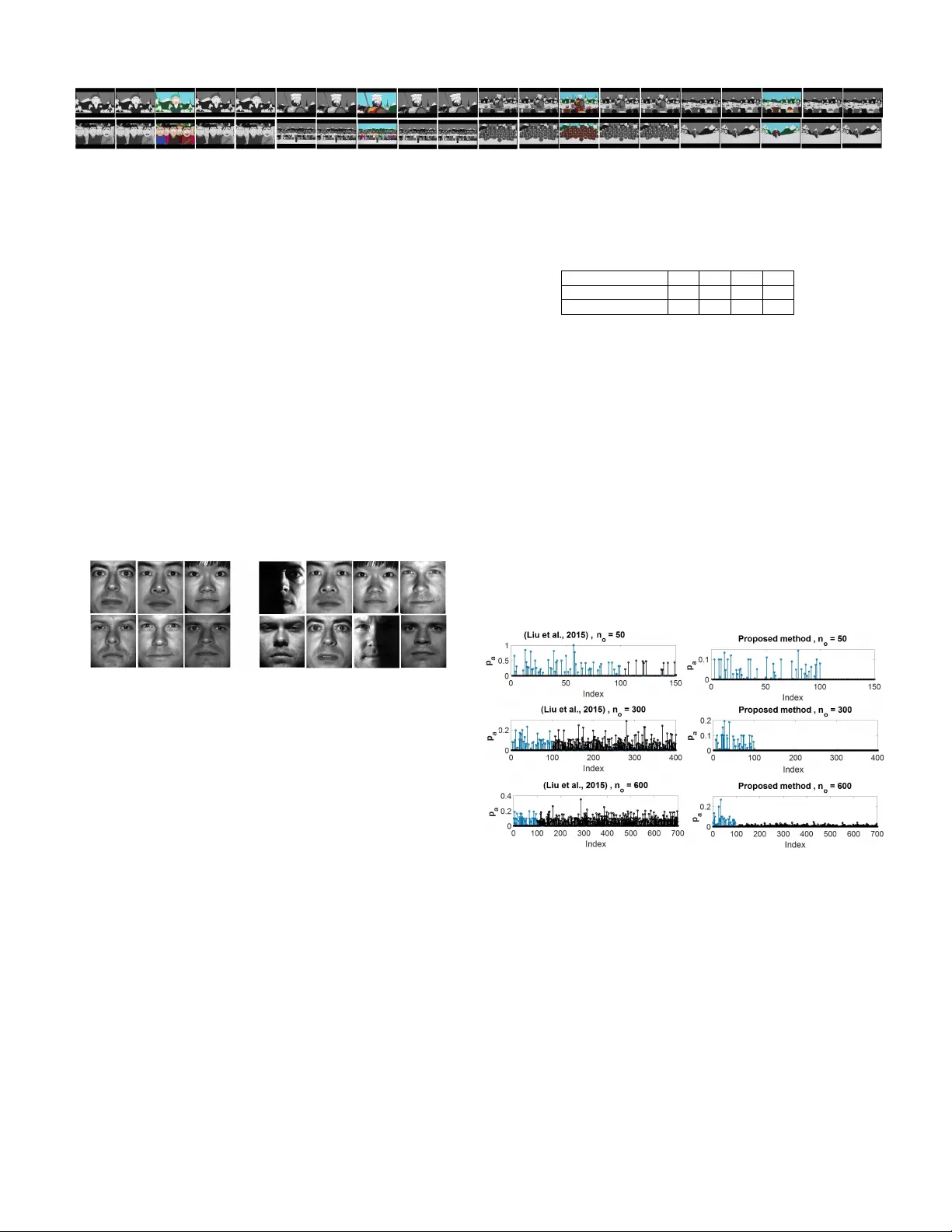
Loading comments...
Leave a Comment