Automatic Node Selection for Deep Neural Networks using Group Lasso Regularization

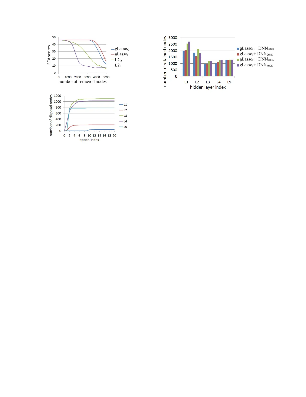
A UT OMA TIC NODE SELE CTION FOR DEEP NEURAL NETWORKS USING GR O UP LASSO REGULARIZA TION Tsubasa Ochiai 1 , ∗ , Shigeki Matsuda 1 , Hideyuki W atanabe 2 , and Shigeru Katagiri 1 1 Graduate School of Science and Engineering, Doshisha Unive rsity , Kyoto, Japan 2 Advanced T elecomm unications Research Institute International, K yo to, Japan ∗ eup1105@mail4 .doshisha.ac.jp ABSTRA CT W e examine the ef fect of the Group Lasso (gLasso) regularizer in selecting the salient nodes of Deep Neural Network (DNN) hidden layers by applying a DNN-HMM hybrid speech recognizer to TED T alks speec h data. W e test two types of gLasso regularization, one for outgoing weight ve ctors and another for incoming w eight vec- tors, as well as two si zes of DNNs: 2048 hidden layer nodes and 4096 nodes. Furthermore, we compare gLasso and L2 regularizers. Our e xperiment results de monstrate that o ur DNN training, in which the gLasso re gularizer was embed ded, successfully selected the hid- den layer nodes that are nece ssary and suf ficient for achieving high classification po wer . Index T erms — Deep neural netw orks, Group Lasso regulariza- tion, Speech recognition 1. INTRODUCTION Moti v ated by the recent rise of Deep Neural Networks (DNNs), we studied their utility for speech recognition by de veloping DNN- HMM hybrid speech recognizers [1, 2]. A DNN’ s high capability is mainly deri ved from a deep layer structure and a massiv e amoun t of network weight parameters. Therefore, rough ly speak ing, the larger and deeper the network, the higher i ts performances are. H o we ver , a larg e network is ob viously undesirable from the viewpoints of computational load an d memory size; it is also un fav orable from the vie wpoint of controlling training rob ustness to unse en data. T o meet this requirement for finding a small, necessary , and sufficient DNN structure, se veral approaches h av e reshaped the network st ructure [3, 4, 5] or pruned the network nodes [6]. Ho wev er, these meth- ods assumed retraining or adapting a size-reduced netwo rk for high discriminativ e power . Therefore, a need obv iously exists for de vel- oping training methods that can automatically (without additional retraining and adaptation) find a small but suf ficient DNN structure. Seeking such de velop ment, we propose in this paper a new train- ing scheme that embeds group L asso (gLasso) regularization [7, 8] for hidden lay er weight v ectors. T o examin e its feasibility , we imple- ment i t in a large-sca le DNN-HMM speech recognizer and cond uct v arious e v aluation experiments in a difficu lt task: TE D T al ks. Quite recently , a gLasso -based idea similar to ours was reported [9]. Howe ver , we independ ently studied it and elaborated the char- acteristics of its scheme in large -scale ex periments. In Section 4, we will discuss the relationship between our work and related works, including [9]. This work was supported in part by JSPS Grants-in-Aid for Scientific Researc h No. 26280063 , MEXT -Supporte d Program “Dri ver-in-t he-Loop, ” and Grant-i n-Aid for JSPS Fello ws. (a) Outgoing (b) Incoming Fig. 1 . Schematic explanation of outgoing/incoming weight vector grouping. 2. DEEP NEURAL NETWORK TRAINING ASSOCIA TED WITH NODE SELECTION 2.1. Computational Procedur es in DNNs W e consider a standard L -layer DNN, where the 0 th layer is an input layer , the L -th lay er is an outpu t layer , and the 1 st throu gh ( L − 1) -th layers are hidden layers. In this network, the l -th layer consists of N l nodes, each of which is associated with a bias coefficient. The nodes are also fully connected among the adjacent l ayers, and each connection is associated with a weight parameter . When a vector pattern is giv en to t he input layer, the network feeds the data fr om the input layer to the output layer in t he following layer-by-lay er manner: a l = W l z l − 1 + b l , and z l = σ ( a l ) , (1) where W l is the weight matrix between the ( l − 1) -th and l -th lay- ers, b l is the bias vector of the l -th layer, z l − 1 is the output vector from the ( l − 1) -th layer , a l is the activ ation vector in the l -th layer, and σ ( ) i s an activ ation function. Here, the i -t h row and j -th col- umn elemen t of W l are w l ij , which is the weight parameter between the j -th node of the ( l − 1) -th l ayer and the i -th node of the l -th layer; the vectors are detailed as follows: a l = [ a l 1 · · · a l i · · · a l N l ] , z l − 1 = [ z l − 1 1 · · · z l − 1 j · · · z l − 1 N l − 1 ] and b l = [ b l 1 · · · b l i · · · b l N l ] , where a l i , z l − 1 j , and b l i are respectively t he aggregated input to the i -th node of the l - th layer , the o utput from the j -th node of the ( l − 1) -th layer, and the bias of the i -th node of the l -th layer . 2.2. Node Selection without Activ ation Changes Figure 1 illustrates an example situation of the n ode connec tions be- tween the ( l − 1) -th layer (of the 2 nodes) and l -t h layer (of t he 2 nodes). As sho wn on its left and right si des, we can basically group the connections i n two ways: 1) outgoing bun dle or 2 ) incoming bun- dle. Based on the se groupin gs, we further grou p their correspon ding weights in outgoing weight v ectors ( w l 1 and w l 2 ) or inco ming weight vectors ( ˜ w l 1 and ˜ w l 2 ). Here, the outgoing weight vectors are column vectors, which form the columns of weight matrix W l ; the incoming weight vectors form the ro ws of W l . In t he figure, for examp le, if the norm of w l 2 is nearly zero and the norm for w l 1 exceed s zero, a l is essentially based only on z l − 1 1 , i.e., the outputs f rom the 1 st ( ν l − 1 1 ) node in the ( l − 1) -th layer . In this situation, e ven if we remo ve node ν l − 1 2 , a l has no large changes an d retains the DNN performances that were gained before node pruning. On the other hand, again for example, if the norm of ˜ w l 2 is nearly zero and the norm for ˜ w l 1 exceed s zero, a ( l +1) is essentially based on z l 1 and b l 2 ( ≈ z l 2 ). In this situation, even if we prune node ν l 2 , a ( l +1) has no large changes and the DNN p erformances according ly remain almost the same. Howe ver , because the node is pruned based on its weight vector norm, its bias remains as a constant. Therefore, we have t o remember he re to shift the bias for the p runed no de to the upper layer node s. As above, regardless of the weight vector grouping, if we can control the values of t he weight vector norm in the DNN training, or more precisely , selecti vely minimize the norm values, we can also achiev e a mechanism that automatically selects nodes wit hout changes in the performances of the trained DNNs. 2.3. DNN T raining with gLas so and L2 Regularizers 2.3.1. Definition of r eg ularized loss The node selection in 2.2 is naturally expected to be done so that only the salient nodes that produce useful outputs for increasing the DNN’ s performances are retained. If DNN training is done to con- currently minimize a loss function that reflects the DNN’ s classifi ca- tion errors and a function that refl ects the norm v alues of the outgo- ing/incoming weight vectors, the unne cessary nodes, which produce useless outputs (for the DNN performances), are automatically dis- abled by their corresponding small norm values and only the sali ent nodes will be retained. T o implement such training, we adopt gLasso regularization for the outgoing or incoming weight vectors in standard DNN training using Cross Entropy (CE) loss. F ocusing on the outgoing weight vector case, we formalize our proposed training scheme belo w . The resulting formalization is basically common to that in the incoming weight vecto r case. Note t hat the target layer for grouping is differen t between types of grouping. Our training scheme st arts by defining regularized loss L ( ) as follo ws: L ( Λ ) = E ( Λ ) + α ˆ R group ( { W l } L l =2 ) + β ˆ R L2 ( W 1 , { b l } L l =1 ) , (2) where Λ is a set of trainable parameters of DNN, i. e., Λ = {{ W l , b l } L l =1 } , E ( ) is the CE loss, ˆ R group ( ) ˆ R L2 ( ) are respec- tiv ely the gLasso and L2 regularizers, and α and β are positiv e constants that con trol the ef fects of the ir correspond ing regularizers. Here the gLasso regularizer is sp ecified as ˆ R group ( { W l } L l =2 ) = L X l =2 R group ( W l ) , (3) where R group ( W l ) = P N l − 1 j =1 k w l j k , and the L2 re gularizer is sp ec- ified as ˆ R L2 ( W 1 , { b l } L l =1 ) = R L2 ( W 1 ) + L X l =1 R L2 ( b l ) , (4) where R L2 ( W l ) = 1 2 k W l k 2 and R L2 ( b l ) = 1 2 k b l k 2 . 2.3.2. Effects of gLasso r e gularization The status of Λ that correspon ds t o the minimum of L ( Λ ) wi ll pro- vides high classifi cation po wer with selected network nodes. T o find that st atus, we minimize L ( Λ ) using the standard gradient-based op- timization procedure. In the above gradient-based loss minimization f or L ( Λ ) , the gra- dient terms of t he regularizers play a key role in accelerating the minimization. In the L2 regularizer case, the gradient of R L2 ( ) is gi ven as follo ws, f or exam ple, in terms of w l j : ∂ R L2 ( W l ) ∂ w l j = w l j . (5) In contrast, the gradient of the gLasso regu larizer becomes ∂ R group ( W l ) ∂ w l j = w l j k w l j k . (6) Eq. (6) clearly indicates the effects of gLasso regularization; the (“outgoing” in this case) weight vector rapidly con verges to zero when its norm is small. As a result, the node outputs, w hich are less useful for the minimization of L ( ) , are disabled in an early stage of the loss minimization, and the retained node outputs will be domi- nantly used for the loss minimization. 2.4. Node Selection Proc edure If the weight v ector norm becomes sufficiently small after the abo ve loss minimization, we can simply prune its corresponding nodes us- ing a threshold value ( θ ). The node selection procedure is summa- rized as follows: 1) calculate the gLasso O norm (column norm) or the gLasso I norm (row norm) for all of the hidden layer nodes, 2) prune t he nodes whose norm v alues are less than θ , and 3) shift the bias for the pruned node to the upper layer nodes, especially in the gLasso I case. (See 3.2 for the definitions of gLasso O and gLasso I .) 3. EXPERIMENTS 3.1. Settings T o ev aluate our proposed DNN training and nod e selection method, we condu cted speech recognition experiments using our DNN- HMM hyb rid spee ch recognizer o ver a TED T alks co rpus that consists of lecture speech data spoke n by 793 speakers. For the e v aluation experiments, we div ided the data into the following three sets: training data by 774 speakers, v alidation data by 8 speakers, and testing data by 11 speakers. The t otal length of the training d ata was about 62 hours, the number of senone classes was 3,944, and the vocab ulary size was 179 , 604 . W e represented the input speech as a series of acoustic feature vectors, each of which w as b ased on M el-scale Frequenc y Cepstrum Coef ficients and of 429 dimensions. See [1] for the details of the input pattern definitions. In ou r DNN-HMM hybrid speech recognize r , the front-end DNN part was the 6 -layer Multi- Layer Perceptron ( L = 6 in 2.1) with a sigmoid acti vation function, and the post-end HMM part used a context-de pendent acoustic model and a 3-gram language model. W e i nitialized the DNN part by the RBM pre-training [10]. Independe ntly of the DNN part, we dev eloped a HMM part using Boosted MMI training [11]. The main targ et of our DNN training was to increase the senon e classification accuracy (SCA), whose categories were indicated by the DNN outputs. Ho wever , we also ev aluated the t raining results using the word error rate (WER) obtained by the post-end HMM part of the hybrid recognizer . T able 1 . Achieved classification performan ces ( %) in DNN 2048 Regularizer SCA B WER B SCA A WER A gLasso O 46.2 18.7 46. 2 18.8 gLasso I 46.1 18.2 46. 1 18.2 L2 O 45.9 18.6 22. 8 42.6 L2 I 45.9 18.6 8.2 100. 0 3.2. Ev aluation procedures W e ran gradient-based t raining for minimizing L ( ) in (2) se veral times, along wi th changing suc h hype r-parameters a s α and β in (2). Ne vertheless, for simplicity , we restricted β t o β = 0 . 1 α or β = 0 . In e very training run, we repeated twenty epochs, in each of which the whole set of training samples was used only once. Among the differe nt trained statuses of Λ , we selected the one that p roduced the highest SCA value o ver t he v alidation data, ev aluated the SCA v al- ues for the selected status of Λ ov er the testing data, and measured the WER values ove r the testi ng data using the selected DNN in t he hybrid recogn izer . In addition to expe riments with our proposed training associ- ated with the gLasso re gularizer , we also tested (for comparison pur- poses) the training using the L2 reg ularizer for all of the weight ma- trixes and all of the bias vectors. Then, the loss i n (2 ) was replaced in this additional case by L ( Λ ) = E ( Λ ) + β L X l =1 n R L2 ( W l ) + R L2 ( b l ) o . (7) T o elaborate the effects of our proposed training method, we also tested two dif ferent DNN sizes: one with 2048 nodes for ev - ery hidden layer (DNN 2048 ) and another with 4096 nodes for ev ery hidden layer (DNN 4096 ). For both DNN 2048 and DNN 4096 , we e v al- uated the following four types of training: 1) with the gLasso reg- ularizer for the outgoing hidden layer weight vectors (gLasso O ), 2) with the gLasso regularizer for the incoming hidden layer w eight vectors ( gLasso I ), 3) with the L2 regularizer for the outgoing hid- den layer weight vectors (L2 O ), and 4) with the L2 r egu larizer for the incoming hidden layer wei ght vectors (L2 I ). Particularly in the L2 O and L 2 I cases, we conducted common L2-regularized training (which corresponds to the training using ( 7)) but selected different nodes, based on the dif ferences in grouping. Moreo ver , as stated in 2.3, we used in all four cases the L2 regu larizer for all of the bias vectors; W e also used the L2 regularizer f or the input l ayer weights in the gLasso O case, and for the output layer wei ghts in the gLasso I case. For con venien ce, we collectiv ely refer to both the gLasso O and gLasso I training cases as gLasso and L2 for both the L2 O and L 2 I cases. 3.3. Results 3.3.1. Funda mental performances In T able 1, we summarize the S CA and WER valu es that we achie ved for D NN 2048 in t he four tr aining cases: gLasso O , gLasso I , L2 O , and L2 I . SCA B and WER B represent the SCA and WE R values (%), both obtained before t he node selection; the SCA and WER values were obtained after the node selection for SCA A and WER A . First, we focus on the results in the SCA B and WE R B columns. Regardless of the weight vector grouping type and t he regularizer type, DNN training achiev ed such accurate classification perfor- mances as an SCA of about 46% and a WER less than 19% . T hey also sho w that the gLasso procedures achie ved the performance that were competitive with the L2 procedures, which are wi dely used in the neural network training. Fig. 2 . Histogram of outgoing weight vec tor norm v alues in gLasso O or L2 O cases. Training was done for DNN 2048 . T op: gLasso O , Bot- tom: L2 O . Next, we observe the characteristics of the weight vector norm v alues that were obtained by the training. Figure 2 shows a his- togram of the outgoing weight vector norm va lues in t he gLasso O or L 2 O cases for DNN 2048 . T he horizontal axis indicates the weight vector norm v alue, and t he vertical axis indicates the freq uency of its correspondin g norm value. From this fi gure, we obtained the follo w- ing findings: 1) The weight vec tor no rm v alues by the gLasso O cases were clearly separated into two groups, suggesting the ease with which the threshold ( θ ) can be set f or the node selection between them; 2) The weight vector norm v alues reduced by t he gLasso O pro- cedure were rather small (at most slightly larger than 10 − 4 ). This distinct reduction proves that the gLasso O process successfully re- duced the norm v alues of some selected weight vectors. 3) The weight vector norm values by the L2 O case were concentrated in the region between 10 0 and 10 1 . This implies that the L 2 procedu re failed to reduce the weight vec tor norm v alues. Due to space limit ations, we omit the introduction of the results in the gLasso I and L 2 I cases. Ho wever , we obtained norm value distribution that c losely resembled that in Figure 2. W e return to T able 1 and compare the results in the SCA B and WER B columns with those in the SCA A and WER A columns. W e executed node selection by setting θ to 10 − 2 , which is clearly f ar from the norm v alues in either of the two separate regio ns generated by the gLasso training. Using this threshold, we pruned 3161 nodes from the fiv e hidden layers in the gLasso O case (the number of retained hidden layer nodes = 7079) and 3368 nodes in the gLasso I (number of retained hidden layer nodes = 6872) case. The performances gained after the node selection (in t he SCA A and WER A columns) are basically the same wi th those gained before the node selection (in the SCA B and WER B columns). The com- parison here clearly prov es that, regardless of the type of weight vector grouping, gLasso training sorted out the weight vectors by selectiv ely r educing the norm values for some weight vectors and allowe d node selection simply based on thresholding. As Figure 2 shows, pruning a certain amount o f nodes is not easy from L2-based DNNs by setting a threshold. For comparison, we remov ed (in ascending order) the small-norm nodes from the DNN produced by the common L2-regularized training in the L2 O case until the number of remo ved nodes became identical to the gLasso O case: 3161; similarly , in the L2 I case, we remov ed 3368 nod es from the L2-based DNN, which was the same with the network used in the L2 O case. The scores i n the SCA A and WER A columns of T able 1 were o btained using these size-redu ced L2-based DNNs. They are much worse than those gained before the node selection and clearly sho w that both the L2 O and L 2 I cases failed to sort out the weight vectors (as a result, their correspo nding nodes). T o further analyze the effects of r egu larizer selection, we ob- served the ch anges i n the SCA scores along with grad ually rem oving hidden l ayer nodes, by 100 nodes, in increasing order of t heir norm v alues. Figure 3 sho ws t he SCA scores, each of which is a function Fig. 3 . Effects of reg ularizer selection in node selection in DNN 2048 . Fig. 4 . Number of disposal nodes for every hidden layer as a function of training epoch in gLasso O -based DNN 2048 . of the number of remov ed nodes. In the fi gure, the horizontal axis indicates the number of removed nodes; the S CA scores for the verti- cal ax is. If the nod es do not exist in the small norm v alue region, the SCA scores gradually decrease as nodes are removed . On the other hand, if t he no des exist in the small n orm v alue region, the SCA v al- ues remain high and later decrease. The curves in the figure clearly prov e that the L2 procedure corresponds to the former situation and the gLasso procedure achie ves the latter desirable situation. 3.3.2. Pr operties of gLasso pro cedur e When i ntroducing gLasso’ s training scheme in 2.3, we stated that the disposable nodes are disabled in some early training stage. T o in vestigate this point, we observ ed the numb er of disposable hidden layer nodes for e very hidden layer as a function o f the training epoch. Here we define a disposable node as one whose norm valu e is smaller than 10 − 2 . Figure 4 illustrates the observed numbers for all five hidden l ayers (1st t hrough 5th) of the gLasso O -based DNN 2048 . W e found the follo wing: 1) Node selection was stably realized with the training progress. 2) It occurred in such comparativ ely early epochs as the 1st through 5th epochs. 3) It dominantly occurred in such higher hidden layers as the 3rd and 4th. The results in Figure 4 suggest that the gLasso p rocedure sho ws a trend that mainly reduces the weight vector norm v alues i n the higher hidden layers. T o scrutinize t his trend, in both the DNN 2048 and DNN 4096 cases, we pruned t he disposable nodes using the 10 − 2 threshold and observed the number of selected (retained) nodes for e very hidden layer . Fi gure 5 illustrates those numbers. Re gardless of t he weight vector group ing (outgoing vs. incoming) or the DNN size (DNN 2048 vs. DNN 4096 ), we found that the gLasso procedure suppressed the weight vector norm v alues, specifically i n t he 3rd and 4th h idden layers, and achiev ed a size-reduced and reshaped net- work structure that was shared in all of the tested cases of gLasso O , gLasso I , DNN 2048 , and DNN 4096 . 4. RELA TE D WORK An orthodox approach for the size reduction of a large matrix is to use Singular V alue Decomposition. A large weight matrix in DNN is decompo sed into small matrixes and re-expresse d (in the sense of Fig. 5 . Number of finally retained hidden layer nodes in gLasso O and gLasso I cases. lo w-rank approximation) by replacing the small eigen v alues of the decompose d diagonal matr ix by zero [3, 4]. This approach allows parameter reduction without serious degradation of the original dis- criminativ e po wer of the network. Ho wever , it does not reduce the number of hidden layer nodes, and therefore it is probably insuf fi- cient to achie ve a desirable amount of network parameter reduction, especially in the case of using the netw ork wi th the huge number of hidden layer nodes. For directly pruning the hidden layer nodes, the L1 norm of the weight vec tors was used as an important function. It resembles the weight-grouping-b ased norm t hat we use in our proposed training procedure [6]. Ho we ver , because such mechanism of reducing the norms in the training procedure as ours was not implemented , DNN restructuring had to rely on additional retraining results. T o find a desirable DNN structure, the G enetic Algorithm (GA) has been applied [12]. It has high potential for generating a target structure, but it often needs an enormous amount of computational resources. Compared w ith the above related studies, our proposed training that embeds the gLasso regularizer is ch aracterized by two main ad- v antages: 1) Ev en if no additional training i s conducted, it can easily produce node-prune d DNNs without performance degradation , and 2) its computation time is almost the same as con ventional L2 regu - larization. Moti v ated by the gLasso procedu re defined in linear reg ression [7], an approach simil ar to ours was proposed [9]. The gLasso reg- ularizer was defined for the outgoing vector grouping of DNN and its ef fect was e valuated in v arious small- and midd le-sized tasks th at classify fixed-dimensional patterns. Compared to this work, we stu d- ied in this paper both the incoming and outgoing vector groupings and also elaborated our proposed scheme in a large -scale speech recognition en vironment. Here, incoming vector grouping can be considered a filtering function and will be appropriate for node se- lection or restructuring for Con volutional Neural Networks. 5. CONCLUSION W e i n vestigated the feasibili ty of the gLasso procedure, i.e., DN N training associated with the gLasso regularizer , for hidden layer weight vectors i n a large-scale speech recognition task with the DNN-HMM hybrid speech recognizer in a T ED T alks task. W e elab- orated the nature of gLasso t raining by applying it to both outgoing and incoming weight vector groupings and compared the gLasso and L2 procedures, where the L2 regularizer was used for all of the weight matr ixes and all of the bias vectors. F rom t he experiment results, we clearly demon strated that our gLasso procedu re auto- matically (without additional t raining) disabled less useful hidden layer nodes wi thout degradation i n DNN cl assification performance and successfully produced a small, necessary , and suf ficient DNN structure. 6. REFERENCES [1] T . Ochiai, S. Matsuda, X. Lu, C. Hori, and S. Katagiri, “Speaker adapti ve training using deep neural networks, ” i n Proc. ICASSP , 2014, pp. 6349-63 53. [2] T . Ochiai, S. Matsuda, H. W atanabe, X. Lu, C. Hori, and S. Katagiri, “Speaker adapti ve training for deep neural networks embedding linear transformation netw orks, ” in Proc. ICASSP , 2015, pp. 4605 -4609. [3] J. Xue, J. Li, and Y . Gong, “Restructuring of deep neural net- work acoustic models with singular value decomposition, ” in Proc. INTERSPPE CH, 2013, pp. 2365-2369. [4] J. Xue, J. L i, D. Y u, M. Seltzer, and Y . Gong, “Singular v al ue decomposition based lo w-footprint sp eaker adaptation an d per- sonalization for deep neural network, ” in Proc. ICAS SP , 2014, pp. 6359-63 63. [5] T . Ochiai, S. Matsuda, H. W atanab e, X. Lu, H. Kaw ai, and S. Katagiri, “Bottleneck linear transformation ne twork adaptation for sp eaker adapti ve training-based hy brid DNN-HMM speech recognizer , ” in Proc. ICASS P , 2016 , pp. 5015-5019. [6] T . He, Y . Fan, Y . Qian, T . T an, and Kai Y u, “Reshaping deep neural network for fast decoding by node-pruning, ” in Proc. ICASSP , 2014, pp. 245-249. [7] M. Y uan and Y . Lin, “Mode l selection and estimation in regres- sion with grouped variables, ” Journal of the Royal Statistical Society: Series B (Stati stical M ethodology), vol. 68, no. 1, pp. 49-67, 2006 . [8] N. Simon, J. Friedman, T . Hastie, and R. T i bshirani, “ A sparse- group lasso” Journal of Computational and Graphical Statis- tics, vol. 2 2, no. 2, pp. 231-245, 2013. [9] S. S cardapan e, Danilo Comminiello, Amir Hussain, and Au- relio Uncini, “Group Sparse Regularization for Deep Neural Networks, ” arXi v:1607.00485v1 (2016). [10] G. E. Hinton, S. Osindero, and Y . T eh, “ A fast learning algo- rithm for deep belief nets, ” Neural Computation, vol. 18, pp. 1527-155 4, 200 6. [11] D. Pov ey , D. Kanev sky , B. Kingsbu ry , B. Ramabhadran, G. Saon, and K. Viswesw ari ah, “Boosted MMI for model and fea- ture sp ace discriminati ve training , ” in Proc. ICASSP , 20 08, pp. 4057-406 0. [12] T . Shinozaki and S. W atanabe, “S tructure discov ery of deep neural netwo rk based on e volutionary algorithms, ” in Proc. ICASSP , 2015, pp. 4979-4983.