Distances and Riemannian metrics for multivariate spectral densities

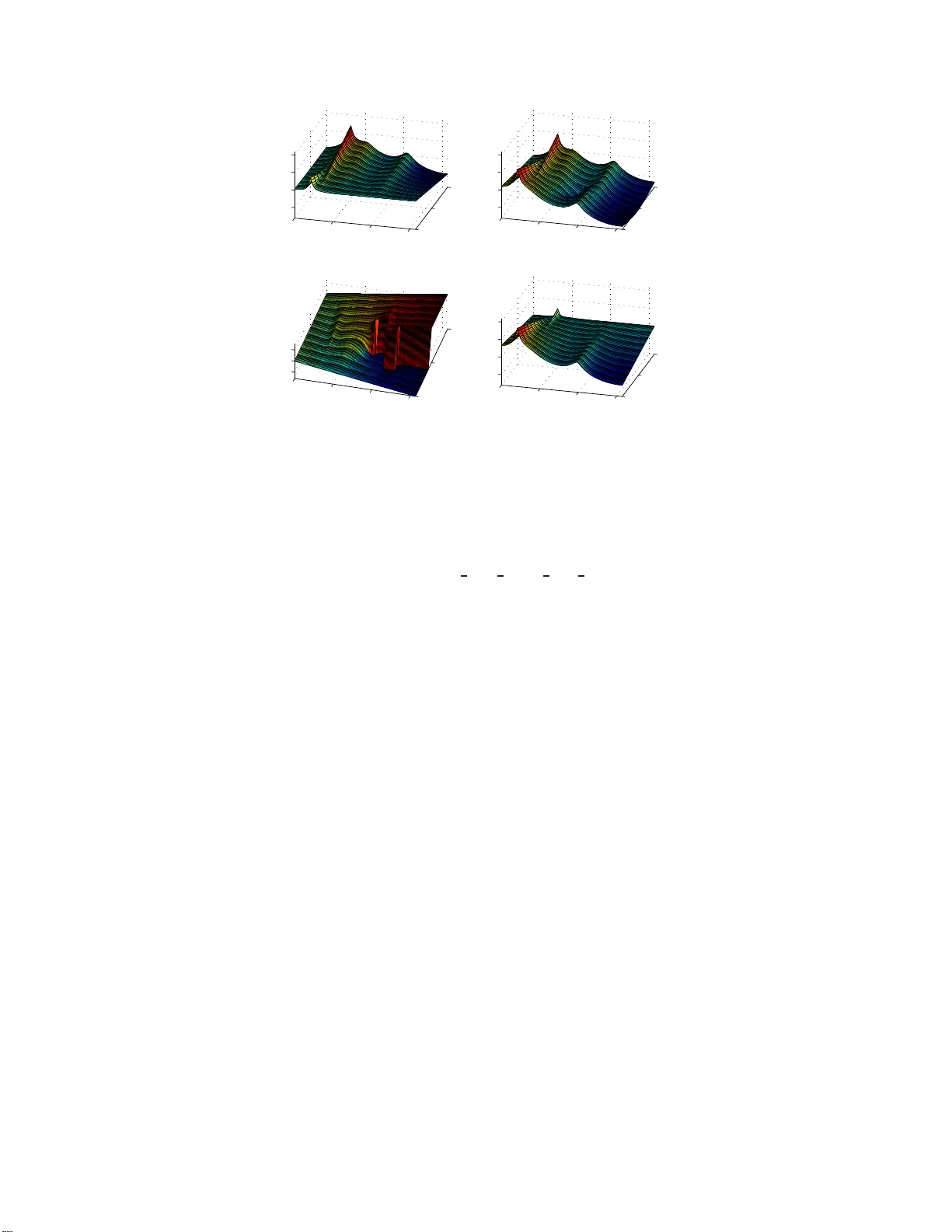
NO VEMBER 26, 2024 1 Distances and Riema nnian metrics for multi v ariate s pectral densitie s Xianhua Jiang, Lipeng Ning, a nd T ryphon T . Geor giou, F ellow , IEEE Abstract W e fir st introdu ce a class of divergence measures between power spectral density m atrices. These are d eriv ed by comparin g the suitability of different models in the co ntext of optimal pr ediction. Distan ces b etween “infinitesimally close” power s pectra are quadratic, and hence, they induce a differential-geom etric stru cture. W e st udy th e corre- sponding R iemann ian metrics and , for a particula r case, provide explicit for mulae for th e corre sponding g eodesics and geodesic distances. The close connec tion between the geom etry of p ower spectra and the geom etry of the Fisher-Rao me tric is no ted. I . I N T R O D U C T I O N Distance measures between s tatistical models an d between s ignals constitute so me o f the ba sic too ls of Signal Processing , System Identification, and Control [1], [2]. Indeed , quantifying dissimilarities is the e ssence of detection, tracking, pattern recognition, model v alidation, signal classification, etc. Naturally , a vari ety of choices are readily av ailable for compa ring de terministic signals and systems . Thes e include various L p and Sobolev norms on signal space s, and indu ced norms in space s of sy stems. Statistical models on the other hand are not elements of a linear space . Their geometry is dictated by positi vity constraints and h ence, they lie on suitable cones or simplices. This is the case for c ov ariances , histog rams, probability distributions, or po wer spe ctra, as t hese n eed to be positiv e in a suitable se nse. A classica l theory for s tatistical mo dels, ha ving r oots in the work of C.R. Rao and R.A. Fisher , is no w kn own as “information ge ometry” [3], [4], [5], [6]. Th e pres ent work aims at a geometric theory s uitable for time-se ries mode led by power spectra. T o this en d, we follow a largely parallel route to that of information geometry (see [7]) in that a metric is now d ictated by the diss imilarit y of models in the context of p rediction theo ry for second -order stocha stic proc esses . The present work buil ds on [7], which focused on sca lar time-series, and is dev oted to power spe ctral densities of multi v ariable s tochastic processe s. The ne ed to compare two power spectra densities f 1 , f 2 directly ha s led to a numbe r of diver gence measures which have been s uggested at various times [1], [2 ]. Ke y among those are the Itakura-Saito dis tance D IS ( f 1 , f 2 ) := Z π − π  f 1 ( θ ) f 2 ( θ ) − log f 1 ( θ ) f 2 ( θ ) − 1  dθ 2 π and the logarithmic spe ctral de viation D log ( f 1 , f 2 ) := s Z π − π     log f 1 ( θ ) f 2 ( θ )     2 dθ 2 π , see e.g., [2, page 370]. The distance measures de veloped in [7] are c losely related to bo th of the se, and the development herein provides a mu lti v ariable counterpart. Indeed, the diver gences that we list between ma trix- valued power spe ctra are s imilar to the Itakura-Saito di ver gence and geodesics on the corresponding Riemannian manifolds of power spectra take the form of logarithmic integrals. Distances between multiv ariable power spec tra have only rece ntly received any attention. In this direc tion we mention generalizations of the Hell inger and It akura-Saito distances by Ferrante et al. [8], [9] and the u se of the Umegaki-von Neumann relative entropy [10]. The goal of this p aper i s to generalize the geometric framework in [7] to the matrix-valued power spectra. W e c ompare two power s pectra in the context of linear prediction: a ch oice between the two is used to design a n o ptimal filter which is then a pplied to a p rocess co rresponding to the sec ond power spectrum. The “flatness” of the innovations process , as we ll as t he degradation of the prediction e rror v ariance, Supported by NSF , AFOSR, and the V incentine Hermes-Luh Endowment. The authors are with the Department of Electrical & Computer Engineering, Univ ersity of Minnesota, Minneap olis, MN 55455. { ji ang082 , ningx015, tryphon } @umn.edu 2 NO VEMBER 26, 2024 when compared to the be st pos sible, are us ed to quan tify the mismatch between the two. This rationale provides us with natural di ver gence measu res. W e then identify c orresponding Riemannian metrics that dictate the underlying geometry . For a certain c ase we compute closed-form express ions for the ind uced g eodesics and ge odesic d istances. These provide a multiv ariable counterpart to the logarithmic intervals in [7] and the logarithmic sp ectral d eviati on [2, page 370]. It is noted that the geo desic distance has certain natural de sirable properties; it is in verse-in variant and congruenc e-in v ariant. Moreover , the manifold of the multi vari ate spec tral den sity func tions endowed with this geodes ic distance is a complete me tric space. A discrete coun ter p art of ce rtain of t hese Riemannian metrics, on the manifold of positiv e definite ma trices (equi valent to p ower spectra which are constant across frequencies ), has been studied extens i vely in connection to the geometry of positi ve o perators [11] and relates to the Rao-Fishe r geometry on probability mode ls restricted to the case of Gaus sian random vectors. Indeed, there is a d eep c onnection betwe en the Itakura-Saito distan ce and the Kullback-Leibler d i ver genc e between the corresp onding probability models [2, page 3 71], [12] which pro vides a link to information geometry . Hence, the Riemann ian ge ometry on power spec tral de nsities in [7] as well as the mu lti v ariable structure pres ented herein is expected to have a strong conne ction als o to the Fisher-Rao metric and the g eometry of information. An interesting stud y in this direction which taps o n an interpretation of the ge ometry of power spectra via the underlying probab ility structure and its c onnection to the Kullback-Leibler di ver gence is given in Y u and Mehta [13]. Ho wever , a transpa rent differential g eometric explanation which highlights points of co ntact is s till to be developed. Further key developments which parallel the framew ork repo rted he rein and are focuse d on momen t problems are presen ted in [8] , [9]. The pa per is or ganized a s follows. In S ection II we estab lish notation an d overvie w the theory of the multi variate quadratic o ptimal prediction problem. In Section III we introduc e alternati ve distan ce measures between multi vari- able power spectra which refle ct mismatch in the context of one-step-ahea d prediction. In Section IV we discuss Riemannian metrics that are indu ced by the diver gence measures of the previous s ection. In S ection V we d iscuss the g eometry of positi ve matrices. In Se ction VI the geo metric structure is a nalyzed an d geode sics a re identified . In Section VII we provide examples to highlight the nature of geod esics betwee n power spectra and ho w these may compare to alternativ es. I I . P R E L I M I N A R I E S O N M U LT I V A R I A T E P R E D I C T I O N Consider a multi v ariate discrete-time, ze ro mean, weakly stationary stoc hastic process { u ( k ) , k ∈ Z } with u ( k ) taking v alues in C m × 1 . Throughout, boldf ace denotes random v ariables/vectors, E de notes expectation, j = √ − 1 the imaginary unit, an d ∗ the complex conjugate transpose. Let R k = E { u ( ℓ ) u ∗ ( ℓ − k ) } for l , k ∈ Z denote the seq uence of matrix cov ariances and dµ ( θ ) be the correspond ing matricial power s pectral measure for which R k = Z π − π e − j k θ dµ ( θ ) 2 π . For the most pa rt, we will be concerned with the case of non -deterministic proce sses with an a bsolutely co ntinuous power spe ctrum. He nce, unless we spe cifically ind icate o therwise, dµ ( θ ) = f ( θ ) dθ with f ( θ ) being a ma trix-v alued power spe ctral density (PSD) function. Further , for a non-deterministic process log ( f ( θ )) nee ds to be integrable, and this will be a ssumed throughout as well. Our interest is in comparing PSD’ s an d in study ing pos sible me trics b etween such. The evident goal is to provide a mean s to quantify deviations and uncertainty in the spec tral domain in a way that is cons istent with particular a pplications. More spec ifically , we presen t metrizations of the spa ce of PSD’ s which are dictated by optimal prediction and reflec t dissimilarit ies that hav e an impact on the qu ality o f prediction. A. Geome try of multivariable pr ocesses W e will be considering least-variance linear prediction problems. T o this en d, we de fine L 2 , u to be the closure of m × 1 -v ector-v alued fin ite linear combinations of { u ( k ) } with respec t to c over gence in the mean [14 , pg . 135]: L 2 , u := ( X finite P k u ( − k ) : P k ∈ C m × m , k ∈ Z ) . NO VEMBER 26, 2024 3 Here, “b ar” denotes closu re. The indice s in P k and u ( − k ) run in opposite directions s o as to simplify the notation later on where prediction is b ased o n past obse rv ations. This space is endowed with b oth, a ma tricial inner produc t [ [ X k P k u ( − k ) , X k Q k u ( − k ) ] ] := E ( X k P k u ( − k ) ! X k Q k u ( − k ) ! ∗ ) , as well as a s calar inner product h X k P k u ( − k ) , X k Q k u ( − k ) i := tr [ [ X k P k u ( − k ) , X k Q k u ( − k ) ] ] . Throughou t, “ tr ” d enotes the trace of a ma trix. It is standard to es tablish the corresponde nce betwee n p := p ( u ) := X k P k u ( − k ) an d p ( z ) := X k P k z k with z = e j θ for θ ∈ [ − π , π ] . This is the K olmogorov iso morphism betwee n the “temporal” space L 2 ( u ) and “spec tral” spa ce L 2 ,dµ , ϕ : L 2 ( u ) → L 2 ,dµ : X k P k u ( − k ) 7→ X k P k z k . It is conv enient to endow the latter space L 2 ,dµ with the matricial inne r product [ [ p, q ] ] dµ := Z π − π  p ( e j θ ) dµ ( θ ) 2 π q ( e j θ ) ∗  as well as the s calar inner product h p, q i dµ := tr [ [ p, q ] ] dµ . The additional structure due to the matricial inner product is often referred to a s Hilber tian (as oppose d to Hilbert ) [15]. Throughou t, p ( e j θ ) = P k P k e j k θ , q ( e j θ ) = P k Q k e j k θ , where we use lo wer case p, q for matrix functions and upper case P k , Q k for the ir matrix coefficients. For no n-deterministic processe s with ab solutely c ontinuous spectral measure dµ ( θ ) = f ( θ ) dθ , we simplify the no tation into [ [ p, q ] ] f := [ [ p, q ] ] f dθ , and h p, q i f := h p, q i f dθ . Least-variance linear p rediction min ( tr E { pp ∗ } : p = u (0) − X k > 0 P k u ( − k ) , P k ∈ C m × m ) (1) can be express ed equ i valently in the spe ctral domain min ( [ [ p, p ] ] f : p ( z ) = I − X k > 0 P k z k , P k ∈ C m × m ) (2) where the minimum is sought in the po siti ve-definite sense , see [15, pg. 35 4], [14, p g. 143]. W e use “ I ” to denote the identity matrix of su itable size . It holds that, although non-negati ve de finiteness define s only a pa rtial orde r on the cone of non -negati ve d efinite Hermitian matrices, a minimizer for (1) a lw ays exists. Of course this corres ponds to a minimizer for (2). The existence of a minimizer is due to the fact that tr E { pp ∗ } is matrix-con vex. He re 4 NO VEMBER 26, 2024 dµ = f dθ is an absolutely continuous measure a nd the quadratic form is not degenerate; see [16, Propo sition 1] for a detailed analysis an d a treatment of the singular cas e where µ is a disc rete matrix-valued mea sure. Further , the minimizer of (1) co incides with the minimizer of min ( h p, p i f : p ( z ) = I − X k > 0 P k z k , P k ∈ C m × m ) . (3) From here on, to kee p notation simple, p ( z ) will de note the minimizer of such a problem, with f specified accordingly , and the minimal matr ix of (1) will be denoted by Ω . That is, Ω := [ [ p, p ] ] f while the minimal value of (3) is tr Ω . The minimizer p is prec isely the image unde r the Kolmogoro v isomo rphism of the optimal prediction e rr or p a nd Ω the prediction-err or variance . B. Spe c tral factors and optimal prediction For a no n-deterministic process the error variance Ω has full rank. Eq ui valently , the product of its eigen v alues is non-zero. The well-known Szeg ¨ o-K olmogorov formula [15, pg. 36 9] det Ω = exp { Z π − π log det f ( θ ) dθ 2 π } (4) relates the produc t of the eige n v alues of the optimal one -step-ahead prediction error variance with the correspond ing PSD. No express ion is avail able in general that would relate f to Ω directly in the matricial ca se. W e consider on ly non-deterministic proces ses a nd hence we assu me tha t log det f ( θ ) ∈ L 1 [ − π , π ] . In this cas e, f ( θ ) admits a un ique factorization f ( θ ) = f + ( e j θ ) f + ( e j θ ) ∗ , (5) with f + ( e j θ ) ∈ H m × m 2 ( D ) , det( f + ( z )) 6 = 0 in D := { z : | z | < 1 } , and normalized so that f + (0) = Ω 1 2 . Th roughout, M 1 2 denotes the Hermitian square root of a Hermitian matrix M . The factor f + is known as the canonica l (left) spectral factor . In the case where f is a scalar function ( m = 1 ) the can onical spe ctral f actor is e xplicitly giv en by f + ( z ) = exp  1 2 Z π − π  1 + z e − j θ 1 − z e − j θ  log f ( θ ) dθ 2 π  , | z | < 1 , As usual, H 2 ( D ) de notes the Hardy s pace of functions which a re analytic in the unit disk D with squ are-integrable radial limits. Spec tral factorization p resents an “explicit” expression of the o ptimal prediction error in the f orm p ( z ) = f + (0) f − 1 + ( z ) . (6) Thus, p ( z ) − 1 is a “ normalized” (left) o uter factor of f . Th e terminology “o uter” refers to a (matrix-valued) function g ( e j θ ) for θ ∈ [ − π , π ] that c an be extended into a n analytic function in the open interior of the unit disc D which is also in vertible in D . I t is often standard not t o diff erentiate betwee n su ch a f unction in D and the fun ction on the boundary of radial-limits since these a re u niquely defined from one another . In the engineering literature outer functions are also referred to as “minimum phase. ” Right-outer factors, where f ( θ ) = f + , right ( e j θ ) ∗ f + , right ( e j θ ) instead of (5) relate to a post-diction optimal es timation problem; in this, the presen t value of the proce ss is estimated via linear comb ination o f future v alues (se e e.g., [16]). Only left factorizations will be use d in the pres ent paper . NO VEMBER 26, 2024 5 I I I . C O M P A R I S O N O F P S D ’ S W e present tw o co mplementing viewpoints on how to compare two PSD’ s , f 1 and f 2 . In both, the o ptimal one-step-ahe ad predictor for o ne of the two s tochastic proces ses, is app lied to the other an d compa red to the correspond ing optimal. Th e first is to conside r how “ white” the power spectrum of the innovations’ proc ess is. The seco nd vie wpoint is to compare how the error v ariance degrades with resp ect to the optimal predictor . Either principle provides a f amily of diver gence me asures and a suitable generaliza tion o f the Riemannian geometry of scalar PSD’ s g i ven in [7]. There is a clos e relationship between the two. A. Prediction er rors and innovations pr ocess es Consider two matrix-v alued spectral density functions f 1 and f 2 . Since an optimal filter will be designe d bas ed on one of the two an d then ev aluated with res pect to the other , some notation is in o rder . First, let us use a subs cript to distinguish betwee n two proce sses u i ( k ) , i ∈ { 1 , 2 } , having the f i ’ s as the correspond ing PSD’ s . They are assu med purely nonde terministic, v ector-v alued, and of c ompatible size. The op timal filters in the s pectral domain are p i := argmin { [ [ p, p ] ] f i p (0) = I , and p ∈ H m × m 2 ( D ) } , and their respec ti ve e rror cov ariances Ω i := [ [ p i , p i ] ] f i . Now defi ne Ω i,j := [ [ p j , p j ] ] f i . Clearly , Ω i,j is the v ariance of the prediction error when the filter p j is used on a proces s having power spec trum f i . Indeed, if we se t p i,j := u i (0) − P j, 1 u i ( − 1) − P j, 2 u i ( − 2) − . . . (7) the prediction-error covariance is [ [ p i,j , p i,j ] ] = [ [ p j , p j ] ] f i . The prediction error p i,j can also be thoug ht of as a time-process , indexed at time-instant k ∈ Z , p ij ( k ) := u i ( k ) − P j, 1 u i ( k − 1) − P j, 2 u i ( k − 2) − . . . for i, j ∈ { 1 , 2 } . This is an innovations pr ocess . Cle arly , from stationarity , [ [ p i,i , p i,i ] ] = Ω i , whereas [ [ p i,j , p i,j ] ] ≥ Ω i , since in this c ase p j is subop timal for u i , in gen eral. B. The co lor of innovations and PSD mismatch W e choose to n ormalize the innovations proce sses as follo ws: h i,j ( k ) = Ω − 1 2 j p i,j ( k ) , for k ∈ Z . The K olmogorov isomorphism takes ϕ : h i,j ( k ) 7→ f − 1 j + , with t he expectation/inner- product being that ind uced by f i , and hence , the po wer sp ectral dens ity of the proce ss h i,j ( k ) is f h ij = f − 1 j + f i f −∗ j + , 6 NO VEMBER 26, 2024 where ( · ) −∗ is a shorthand for (( · ) ∗ ) − 1 . When f i = f j , e vidently { h i,i k } is a white noise process with cov ariance matrix equals to the iden tity . Naturally , in an a bsolute sense, the mismatch between the two power spectra f i , f j can be quantified by the distance of f h ij to the identity . T o this end we may con sider any s ymmetrized expression: Z π − π d( f − 1 j + f i f −∗ j + , I ) dθ 2 π + Z π − π d( f − 1 i + f j f −∗ i + , I ) dθ 2 π (8) for a s uitable distance d( · , · ) between pos iti ve de finite matrices. In ge neral, it is deemed desirable that dista nces between power spe ctra are in variant to sc aling (as is the case when distance s depe nd on ratios of sp ectra, [2]). Research ers a nd practitioners alike have insisted on s uch a property , especially for speech a nd image syste ms, due to an a pparent agreemen t with s ubjectiv e q ualities of s ound and images. It is thus interesting to seek a multiv ariable analogue s inheren t in the above compa rison. Due to the no n-negati ve definitenes s of po wer s pectra, a con venient option is to take “ d ” as the trace : Z π − π tr  f − 1 j + f i f −∗ j + − I  + tr  f − 1 i + f j f −∗ i + − I  dθ 2 π . This inde ed defines a distance measure sinc e ( x + x − 1 − 2) is a non -negati ve func tion for 0 < x ∈ R that vanishes only when x = 1 . Thu s, we define D 1 ( f 1 , f 2 ) := Z π − π tr  f − 1 2 f 1 + f − 1 1 f 2 − 2 I  dθ 2 π . (9a) Interestingly , D 1 ( f 1 , f 2 ) ca n b e re-written as follows: D 1 ( f 1 , f 2 ) = Z π − π k f − 1 / 2 1 f 1 / 2 2 − f 1 / 2 1 f − 1 / 2 2 k 2 F r dθ 2 π (9b) where k M k 2 F r := tr M M ∗ denotes the square of the Frobenius n orm 1 . It can be readily verified starting f rom t he right han d side of (9b) and s implifying this to match (9a). It is now be ea sily seen tha t D 1 ( f i , f j ) ha s a numb er of desirable properties listed in the following proposition. Pr oposition 1: Conside r f i , f j being PSD’ s of no n-deterministic proc esses and g ( e j θ ) an arbitrary outer matrix- valued function in H m × m 2 ( D ) . The followi ng h old: (i) D 1 ( f i , f j ) ≥ 0 . (ii) D 1 ( f i , f j ) = 0 if f f i = f j (a.e.). (iii) D 1 ( f i , f j ) = D 1 ( f j , f i ) . (i v) D 1 ( f i , f j ) = D 1 ( f − 1 i , f − 1 j ) . (v) D 1 ( f i , f j ) = D 1 ( g f i g ∗ , g f j g ∗ ) . Pr oof: Properties (i-iv) follow immediately from (9b) while the in variance prope rty (v) is most easily seen by employing (9a). C. Subo ptimal pr ediction a nd PSD mismatch W e now attempt to quantify ho w suboptimal the pe rformance o f a filter is when this is based on the incorrect choice b etween the two alternativ e P SD’ s. T o this e nd, we consider the error c ov ariance and co mpare it to that of the optimal predictor . A basic inequality between these error covariances is su mmarized in the follo wing prop osition. Pr oposition 2: Under our ea rlier standard assu mptions, for i, j ∈ { 1 , 2 } and Ω i , Ω j > 0 , it holds that Ω i,j ≥ Ω i . (10a) Further , the above holds a s an equality if f p i = p j . Pr oof: It follo ws from the optimality o f p i since [ [ p j , p j ] ] f i ≥ [ [ p i , p i ] ] f i = Ω i . 1 √ tr M M ∗ is also referred t o also as the Hi lbert-Schmidt norm. NO VEMBER 26, 2024 7 Cor ollary 3: The following hold: Ω − 1 2 i Ω i,j Ω − 1 2 i ≥ I (10b) det(Ω i,j ) ≥ det(Ω i ) (10c) tr(Ω i,j ) ≥ tr(Ω i ) (10d) Ω − 1 2 j Ω i,j Ω − 1 2 j ≥ Ω − 1 2 j Ω i Ω − 1 2 j . (10e) Further , each “ ≥ ” holds as eq uality if f p i = p j . Thus, a mismatch between the two s pectral den sities can be qua ntified by the streng th of the above inequa lities. T o this e nd, we may cons ider a number of alternati ve “div ergence mea sures”. First we conside r: D 2 ( f i , f j ) := log det  Ω − 1 2 i Ω i,j Ω − 1 2 i  . (11) Equiv alent o ptions leading to the same Riema nnian structure are: 1 m tr(Ω − 1 2 i Ω i,j Ω − 1 2 i ) − 1 , and (12a) det(Ω − 1 2 i Ω i,j Ω − 1 2 i ) − 1 . (12b) Using the gen eralized Szeg ¨ o-K olmogorov expression (4 ) we readily obta in that D 2 ( f i , f j ) = log det  Z π − π f − 1 j + f i f −∗ j + dθ 2 π  − Z π − π log det  f − 1 j + f i f −∗ j +  dθ 2 π (13) = tr  log Z π − π f − 1 j + f i f −∗ j + dθ 2 π − Z π − π log f − 1 j + f i f −∗ j + dθ 2 π  . This e xpress ion takes v alues in [0 , ∞ ] , and is zero if a nd only if the n ormalized spectral factors p − 1 = Ω − 1 / 2 f + are identica l for the two sp ectra. Further , it provides a natural gene ralization of the di vergence mea sures in [7] and of the Itakura dis tance to the case o f multi variable spe ctra. It satisfies “congruence in v ariance. ” Th is is sta ted next. Pr oposition 4: Conside r two PSD’ s f i , f j of non-deterministic process es and g ( e j θ ) an outer matrix-valued function in H m × m 2 ( D ) . The followi ng h old: (i) D 2 ( f i , f j ) ≥ 0 . (ii) D 2 ( f i , f j ) = 0 if f p i = p j . (iii) D 2 ( f i , f j ) = D 2 ( g f i g ∗ , g f j g ∗ ) . Pr oof: P roperties (i-ii) follo w immediately from (11) while the in vari ance p roperty (iii) is most easily seen be employing (13). T o this end, first no te that g f + obviously constitutes the s pectral factor of gf g ∗ . Substituting the correspond ing expression s in (13) e stablishes the in v ariance. D. Alternative dive r gence m e asures Obviously , a lar ge family of div ergence measures between two ma trix-v alued po wer s pectra ca n be obtained based on (8). For completene ss, we sugg est rep resentativ e po ssibilities some of wh ich have been independe ntly considered in rece nt literature. 1) F r obenius dis tan ce: If we use the Frobenius norm in (8) we obtain D F ( f 1 , f 2 ) := 1 2 X i,j Z π − π k f − 1 j + f i f −∗ j + − I k 2 F r dθ 2 π (14a) where P i,j designates the “symmetrized su m” tak ing ( i, j ) ∈ { (1 , 2) , (2 , 1) } . It ’ s straightforw ard to see that all of f − 1 j + f i f −∗ j + , f − 1 2 j f i f − 1 2 j and f − 1 j f i share the same eige n v alues for any θ ∈ [ − π , π ] . Thu s, k f − 1 j + f i f −∗ j + − I k 2 F r = k f − 1 2 j f i f − 1 2 j − I k 2 F r , 8 NO VEMBER 26, 2024 and D F ( f 1 , f 2 ) = 1 2 X i,j Z π − π k f − 1 2 j f i f − 1 2 j − I k 2 F r dθ 2 π . (14b) Obviously (14b) is preferable over (14a) s ince no spectral factorization is in v olved. 2) Hellinger distance : A generaliza tion of the Hellinger distance h as been proposed in [9] for c omparing multi variable sp ectra. B riefly , given two positive definite matrices f 1 and f 2 one see ks factorizations f i = g i g ∗ i so that the integral over frequen cies of the Frobenius distance k g 1 − g 2 k 2 F r between the factors is minimal. The factorization does not need to correspond to an alytic factors. Whe n one of the two sp ectra is the identity , the optimization is trivial a nd the Hellinger distan ce becomes Z π − π k f 1 2 − I k 2 F r dθ 2 π . A variation o f this idea is to compare the normalized innovation spec tra ( f − 1 j + f i f −∗ j + ) 1 2 , for i, j ∈ { 1 , 2 } , to the identity . W e do this in a symmetrized fashion so tha t togethe r with s ymmetry the metric inherits the in verse- in v ariance property . Th us, we define D H ( f 1 , f 2 ) := X i,j Z π − π k ( f − 1 j + f i f −∗ j + ) 1 2 − I k 2 F r dθ 2 π (15) = X i,j Z π − π k ( f − 1 2 j f i f − 1 2 j ) 1 2 − I k 2 F r dθ 2 π . The seco nd equality follo ws by the fact that f j + f − 1 2 j is a frequency-dep endent unitary matrix. 3) Multivariab le Itakura-Saito distanc e: The c lassical Itaku ra-Saito distanc e ca n be rea dily g eneralized by taking d( f , I ) = tr( f − log f − I ) . The values a re alw ays pos iti ve for I 6 = f > 0 an d equal to zero when f = I . Thus, we may de fine D IS ( f 1 , f 2 ) = Z π − π d( f − 1 2+ f 1 f −∗ 2+ , I ) dθ 2 π (16) = Z π − π  tr( f − 1 2 f 1 ) − log det ( f − 1 2 f 1 ) − m  dθ 2 π . The Itakura-Saito distance has its origins in max imum likeli hood e stimation for sp eech processing and is related to the Kullback-Leibler diver gence between the proba bility la ws of tw o Gauss ian random process es [2], [12]. More recently , [8] introdu ced the matrix-version of the Itakura-Sa ito dis tance for so lving the state-covariance matching problem in a multiv ariable setting. 4) Log-spe ctral deviation: It h as been argued tha t a logarithmic measure of spec tral d eviati ons is in ag reement with perceptiv e qualities of sound and for this reason it h as formed the basis for the oldes t distortion measures considered [2]. In particular , the L 2 distance between the logarithms of p ower spectra is referred to as “Lo g-spectral deviation” or the “logarithmic e nergy . ” A na tural multi v ariable version is to cons ider d( f , I ) = k log ( f ) k 2 F r . This expression is already symmetrized , since d( f , I ) = d( f − 1 , I ) by virtue of the fact that the e igen v alues of log( f ) and thos e of log( f − 1 ) differ only in their sign. Thereb y , k log( f − 1 j + f i f −∗ j + ) k 2 F r = k log( f − 1 i + f j f −∗ i + ) k 2 F r . Thus we defin e D Log ( f 1 , f 2 ) := Z π − π k log( f − 1 1+ f 2 f −∗ 1+ ) k 2 F r dθ 2 π (17) = Z π − π k log( f − 1 2 1 f 2 f − 1 2 1 ) k 2 F r dθ 2 π . This represents a multi v ariable version of the log-s pectral de viation (see [2, page 370]). Interestingly , as we will see later on, D Log ( f 1 , f 2 ) possesses several use ful properties a nd, in fact, its sq uare root turns out t o be precise ly a geod esic dis tance in a suitable Riemann ian g eometry . NO VEMBER 26, 2024 9 I V . R I E M A N N I A N S T RU C T U R E O N M U LT I V A R I A T E S P E C T R A Consider a “sma ll” perturbation f + ∆ away from a nominal po wer sp ectral d ensity f . All diver gence measures that we ha ve seen s o far are co ntinuous in t heir ar guments and , in-the-small, c an be app roximated by a quadratic form in ∆ which depend s co ntinuously o n f . This is wha t is referred to a s a Riema nnian metric . Th e av ailability of a metric giv es the s pace of power s pectral dens ities its properties. It dictates how pe rturbations in various directions compare to e ach other . It also provides add itional impo rtant c oncepts: g eodesics , g eodesic distanc es, an d c urvature. Geodes ics a re pa ths of smallest length connecting the start to the fi nish; this length is the ge odesic distance . Thus, geodes ics in the space of power spectral den sities represent de formations from a starting power spectral dens ity f 0 to an end “point” f 1 . Curvature o n the other h and is intimately connected with app roximation and con vexit y of sets. In contrast to a g eneral diver gence meas ure, the geo desic distance obeys the triangular inequ ality and thus, it is a metric (or , a p seudo-metric wh en by design it is un aff ected by scaling or other group of transformations). Geo desics are also natural structures for mod eling c hanges and deformations. In fact, a key motiv ation be hind the present work is to model time-varying spectra via geodes ic paths in a suitable metric spa ce. Th is viewpoint provides a non-parametric model for no n-stationary spectra, analog ous to a s pectrogram, but on e wh ich takes into acco unt the inherent geometry of power spectral densities. Thus, in the s equel we consider infinitesimal perturbations abou t a g i ven power spectral dens ity function. W e explain how these g i ve rise to no nnegativ e definite quad ratic forms. Through out, we assume that all functions a re smooth e nough s o tha t the indica ted integrals exist. This can be e nsured if a ll spe ctral dens ity func tions are bound ed with bounde d d eri vati ves and in verses. Thus, we will restrict our attention to the follo wing class of PDF’ s: F := { f | m × m pos iti ve de finite, dif ferentiable on [ − π , π ] , with continuo us deri vati ve } . In the above, we identify the en d points of [ − π , π ] since f is thought of as a function o n the unit circle. Since the functions f are strictly pos iti ve defi nite and bounded , tangen t directions of F consists of admissible perturbations ∆ . Thes e need only b e restricted to b e diff erentiable w ith squa re integrable d eri vati ve, h ence the tangen t space at any f ∈ F can be ide ntified with D := { ∆ | differentiable on [ − π , π ] with continuous deriv ati ve } . A. Geome try based on the “flatnes s ” o f innovations spectra W e first cons ider the diver gence D 1 in (9a-9b) which quantifies h ow far the PSD of the no rmalized inn ov ations process is from being c onstant and equal to the ide ntity . The induced Riemannian metric takes the form g 1 ,f (∆) := Z π − π k f − 1 / 2 ∆ f − 1 / 2 k 2 F r dθ 2 π . (18a) Pr oposition 5: Let ( f , ∆) ∈ F × D and ǫ > 0 . T hen, for ǫ sufficiently small, D 1 ( f , f + ǫ ∆) = g 1 ,f ( ǫ ∆) + O ( ǫ 3 ) . Pr oof: First note that tr  f ( f + ǫ ∆) − 1  = tr  f 1 / 2 ( I + f − 1 / 2 ǫ ∆ f − 1 / 2 ) − 1 f − 1 / 2  = tr  I + f − 1 / 2 ǫ ∆ f − 1 / 2  − 1 tr  f ( f + ǫ ∆) − 1  = m − tr( f − 1 / 2 ǫ ∆ f − 1 / 2 ) + k f − 1 / 2 ǫ ∆ f − 1 / 2 k 2 F r + O ( ǫ 3 ) . Like wise, tr( f + ǫ ∆) f − 1 = m + tr( ǫ ∆ f − 1 ) = m + tr( f − 1 / 2 ǫ ∆ f − 1 / 2 ) . 10 NO VEMBER 26, 2024 Therefore, D 1 ( f , f + ǫ ∆) = tr Z π − π  f ( f + ǫ ∆) − 1 + ( f + ǫ ∆) f − 1 − 2 I  dθ 2 π = Z π − π k f − 1 / 2 ǫ ∆ f − 1 / 2 k 2 F r dθ 2 π + O ( ǫ 3 ) . Obviously , an alternati ve expres sion for g 1 ,f that requires neither spectral f actorization nor the computation of the Hermitian squ are roo t of f , is the following: g 1 ,f (∆) := Z π − π tr  f − 1 ∆ f − 1 ∆  dθ 2 π . (18b) It is interesting to als o note that any of (14), (15), (16), an d (17) leads to the same Rie mannian metric. B. Geome try based on subop timality of p r ediction The paradigm in [7] for a Riemannian structure of scalar power s pectral dens ities was originally built on the degradation of pre dicti ve error variance, as this is reflected in the strength o f the ine qualities of Propos ition 2. In this section we explore the direct generalization of that route. T hus, we consider the qua dratic form which F inherits from the rele vant diver gence D 2 , defined in (11). The next propo sition s hows that this defines the corresponding metric: g 2 ,f (∆) := tr Z π − π ( f − 1 + ∆ f −∗ + ) 2 dθ 2 π − tr  Z π − π f − 1 + ∆ f −∗ + dθ 2 π  2 = g 1 ,f (∆) − tr  Z π − π f − 1 + ∆ f −∗ + dθ 2 π  2 . (19) Pr oposition 6: Let ( f , ∆) ∈ F × D and ǫ > 0 . T hen, for ǫ sufficiently small, D 2 ( f , f + ǫ ∆) = 1 2 g 2 ,f ( ǫ ∆) + O ( ǫ 3 ) . Pr oof: In order to simplify the nota tion let ∆ ǫ := f − 1 + ǫ ∆ f −∗ + . Since ∆ , f are bo th bou nded, | tr(∆ k ǫ ) | = O ( ǫ k ) as we ll as | tr( R π − π ∆ ǫ dθ 2 π ) k | = O ( ǫ k ) . Using a T ay lor series expansion, tr log  Z π − π f − 1 + ( f + ǫ ∆) f −∗ + dθ 2 π  = tr log  I + Z π − π ∆ ǫ dθ 2 π  = tr  Z π − π ∆ ǫ dθ 2 π  − 1 2 tr  Z π − π ∆ ǫ dθ 2 π  2 + O ( ǫ 3 ) , while tr  Z π − π log( f − 1 + ( f + ǫ ∆) f −∗ + ) dθ 2 π  = Z π − π tr log ( I + ∆ ǫ ) dθ 2 π = Z π − π tr(∆ ǫ − 1 2 ∆ 2 ǫ ) dθ 2 π + O ( ǫ 3 ) . Thus D 2 ( f , f + ǫ ∆) = 1 2 tr  Z π − π ∆ 2 ǫ dθ −  Z π − π ∆ ǫ dθ 2 π  2  + O ( ǫ 3 ) . NO VEMBER 26, 2024 11 Evidently , g 2 ,f and g 1 ,f are close ly related. The o ther choices o f D s imilarly yield either g 1 ,f , as n oted earlier , or g 2 ,f . In fact, g 2 ,f can be deriv ed base d o n (12). W e remark a substantial dif ference between g 1 ,f and g 2 ,f . In contrast to g 2 ,f , ev aluation o f g 1 ,f does not require computing f + . However , on the other hand, b oth g 1 ,f , a nd g 2 ,f are similarl y un af fected by co nsistent sc aling of f and ∆ . V . G E O M E T RY O N P O S I T I V E M A T R I C E S As ind icated earlier , a Riemannian metric g(∆) on the spa ce of Hermitian m × m matrices is a family of quadratic forms originating from inn er products that depend smoothly on the Hermitian “foot point” M —the standard Hilbert-Schmidt metric g HS (∆) = h ∆ , ∆ i := tr(∆ 2 ) being one such. Of p articular interest are metrics on the space of positive d efinite matrices that ensure the spa ce is comple te and geodes ically complete 2 . For our purposes , matrices typically represe nt cov ariances . T o this end a standard recipe for constructing a Riemannian metric is to begin with an information potential, such as the Boltzmann entropy of a Gau ssian distrib ution with zero mean and covariance M , S ( M ) := − 1 2 log(det( M )) + constan t , and define an inner p roduct via its Hess ian h X, Y i M := ∂ 2 ∂ x∂ y S ( M + xX + y Y ) | x =0 ,y =0 = tr( M − 1 X M − 1 Y ) . The Riemannian metric s o defined, g M (∆) : = tr( M − 1 ∆ M − 1 ∆) = k M − 1 2 ∆ M − 1 2 k 2 F r , is none other than the Fisher -Rao metric on Gaus sian distributions expressed in the s pace of the correspo nding covari ance matrices. The relations hip o f the Fishe r -Rao me tric on Ga ussian distributions with the metric g 1 ,f in (18b ) is rather evident. Indeed, g M coincides with g 1 ,f for power sp ectra which are constant across frequencies, i.e., taking f = M to be a cons tant He rmitian positi ve definite matrix. It is noted tha t g M (∆) remains in variant un der congruenc e, that is, g M (∆) = g T M T ∗ ( T ∆ T ∗ ) for any squa re in vertible matrix-function T . Th is is a natural property to demand s ince it implies tha t the distance between covariance matrices does not chang e u nder coordinate transformations. The same is inherited by g 1 ,f for power spectra. It is for this reaso n that g M has in fact bee n extensively studied in the con text of g eneral C ∗ -algebras and the ir p ositi ve elements ; we refer to [11, pg. 201-235 ] for a nice exposition of rele vant material and for further references. Below we highlight certain key facts that are rele vant to this pape r . But fi rst, and for future reference, we recall a sta ndard result in dif ferential geome try . Pr oposition 7: Let M be a Riemannian manifold with k ∆ k 2 M denoting the Riema nnian metric at M ∈ M and ∆ a tangen t direction at M . For ea ch pair of points M 0 , M 1 ∈ M conside r the path s pace Θ M 0 ,M 1 := { M τ : [0 , 1] → M : M τ is a piecewise smooth path conne cting the two given points } . Denote by ˙ M τ := dM τ /dτ . The arc-length Z 1 0 k ˙ M τ k M dτ , 2 A space is complete when Cauchy sequences con v erge to points i n the space. It is geodesically complete when the definition domain of geodesics extends to the complete real line R ; i.e., extrapolating t he path beyo nd the end points remains alw ays in t he space. 12 NO VEMBER 26, 2024 as well as the “ action/energy” functiona l Z 1 0 k ˙ M τ k 2 M dτ attain a minimum a t a common path in Θ f 0 ,f 1 . Further , the minimal value of the arclength is the s quare root of the minimal value of the ene r gy functional, and on a minimi zing p ath the “speed” k ˙ M τ k M remains constan t for τ ∈ [0 , 1] . Pr oof: See [17, pg. 137]. The insight behind the statement o f the p roposition is a s follows. The arclength is evidently un af fected by a re- parametrization of a g eodesic connecting the two points. The “energy” functional on the other hand, is minimized for a spe cific parame trization of geode sic where t he velocity stay s co nstant. Thu s, the two are intimately related. The propo sition will be a pplied first to paths between ma trices, but in the next s ection it will also be in vok ed for geodes ics betwe en po wer spectra. Herein we are interes ted in geodesic pa ths M τ , τ ∈ [0 , 1] , connecting positive definite matrices M 0 to M 1 and in computing the corresp onding geodesic distances d g ( M 0 , M 1 ) = Z 1 0 k M − 1 / 2 τ dM τ dτ M − 1 / 2 τ k F r dτ . Recall that a ge odesic M τ is the shortest path on t he manifold c onnecting the beginning to the end. Theorem 8: Given Hermitian positiv e matrices M 0 , M 1 the g eodesic between the m with res pect to g M is unique (modulo re-parametrization) and given by M τ = M 1 / 2 0 ( M − 1 / 2 0 M 1 M − 1 / 2 0 ) τ M 1 / 2 0 , (20) for 0 ≤ τ ≤ 1 . Further , it holds tha t d g ( M 0 , M τ ) = τ d g ( M 0 , M 1 ) , for τ ∈ [0 , 1] , and the geode sic distance is d g ( M 0 , M 1 ) = k log ( M − 1 / 2 0 M 1 M − 1 / 2 0 ) k F r . Pr oof: A proof is given in [11, Theorem 6.1.6, pg. 205 ]. Howe ver , since this is an important result for our purposes and for completene ss, we provide an indepe ndent sh ort p roof re lying on Po ntryagin’ s minimum principle. W e first note tha t, since g M is con gruence in v ariant, the pa th T M τ T ∗ is a g eodesic between T M 0 T ∗ and T M 1 T ∗ , for any in vertible matrix T . Further , the ge odesic length is indepe ndent of T . Thus , we set T = M − 1 2 0 , and seek a ge odesic path between X 0 = I and X 1 = M − 1 2 0 M 1 M − 1 2 0 . ( 21) Appealing to Proposition 7 we seek min { Z 1 0 tr( X − 1 τ U τ X − 1 τ U τ ) dτ , (22) subject to ˙ X τ = U τ , and X 0 , X 1 specified } . Now , (22) is a standa rd optimal control problem. The value of the optimal c ontrol mus t a nnihilate the variation of the Hamiltonian with respe ct to the “control” U τ tr( X − 1 τ U τ X − 1 τ U τ ) + tr(Λ τ U τ ) . Here, Λ τ represents the co-state (i.e., Lagrange multipli er fun ctions). The variation is tr(2 X − 1 τ U τ X − 1 τ δ U + Λ τ δ U ) NO VEMBER 26, 2024 13 and this being iden tically zero for all δ U implies that U τ = − 1 2 X τ Λ τ X τ . (23) Similarly , the co-state equation is obtaine d b y cons idering the variation with respec t to X . T his gi ves ˙ Λ τ = 2 X − 1 τ U τ X − 1 τ U τ X − 1 τ . Substitute the expression for U τ into the state an d the co-state equations to obtain ˙ X τ = − 1 2 X τ Λ τ X τ ˙ Λ τ = 1 2 Λ τ X τ Λ τ . Note that ˙ X τ Λ τ + X τ ˙ Λ τ = 0 , identically , for all τ . Hence, the product X τ Λ τ is cons tant. Se t X τ Λ τ = − 2 C. (24) The state equa tion becomes ˙ X τ = C X τ . The solution with initial c ondition X 0 = I is X τ = exp( C τ ) . Matching (21) requires tha t exp( C ) = X 1 = M − 1 2 0 M 1 M − 1 2 0 . Thus, X τ = ( M − 1 2 0 M 1 M − 1 2 0 ) τ and the geode sic is as claimed. Further , C = log ( M − 1 2 0 M 1 M − 1 2 0 ) while U τ = C X τ from (24) and (23). So fin ally , for the minimizing cho ice of U τ we get that the cos t Z τ 0 tr( X − 1 τ U τ X − 1 τ U τ ) dτ = Z τ 0 tr( C 2 ) dτ = τ k log ( M − 1 / 2 0 M 1 M − 1 / 2 0 ) k 2 F r as claimed. Remark 9: It’ s important to point out the l ower b ound d g ( M 0 , M 1 ) ≥ k log M 0 − log M 1 k F r (25) on the geodesic distan ce which holds with equality wh en M 0 and M 1 commute. This is kn own as the expone ntial metric increasing prope rty [11, p age 203] and will be u sed later on. 2 The mid point of the g eodesic path in (20) is what is known as the geometric mea n of the two ma trices M 0 and M 1 . This is co mmonly d enoted by M 1 2 := M 0 ♯M 1 . Similar notation, with the a ddition of a subs cript τ , will be used to designate the complete geodesic path M τ = M 0 ♯ τ M 1 := M 1 / 2 0 ( M − 1 / 2 0 M 1 M − 1 / 2 0 ) τ M 1 / 2 0 (see [11]). A numbe r of useful properties can be eas ily veri fied: i) Congrue nce in variance: for any in vertible matrix T , d g ( M 0 , M 1 ) = d g ( T M 0 T ∗ , T M 1 T ∗ ) . ii) In verse in variance: d g ( M 0 , M 1 ) = d g ( M − 1 0 , M − 1 1 ) . 14 NO VEMBER 26, 2024 iii) The metric sa tisfies the semiparallelogram law . i v) The sp ace of positiv e definite matrices metrized by d g is complete; that is, any Cauchy sequ ence o f positi ve definite matrices con verges to a pos iti ve definite matrix. v) Giv en any three “points” M 0 , M 1 , M 2 , d g ( M 0 ♯ τ M 1 , M 0 ♯ τ M 2 ) ≤ τ d g ( M 1 , M 2 ) , which implies that geo desics di ver ge at least as fast as “E uclidean geodes ics”. Remark 10: Property v ) implies that the Riema nnian man ifold o f po siti ve de finite matrices with metri c d g has nonpos iti ve sectional curvature [18, pg. 39–40 ]. The nonpos iti ve sectional curvature of a simply conne cted complete Riemannian manifold has several important geometric conse quence s. It implies the existence and uniqueness of a geodes ic connecting any two points on the manifold [18, p g. 3–4]. Con vex s ets on such a manifold are d efined by the requirement that geo desics between any two points in the set lie entirely in the set [18, pg. 67]. The n, “projec tions” onto the set exist in that the re is a lw ays a closes t point within c on vex se t to any g i ven point. Eviden tly , such a property should be valuable in applications, su ch a s sp eaker identification or speec h recognition b ased o n a da tabase of speech segments; e .g., mode ls may be taken as the “conv ex hull” o f prior sample s pectra and the metric distance of a new samp le compared to how far it resides from a giv en s uch co n vex set. Another prope rty of such a ma nifold is that the center of ma ss of a set of points is co ntained in the clos ure of its con ve x hull [18, pg . 68]; this property has been used to defi ne the geometric means of s ymmetric positi ve matrices in [19]. 2 V I . G E O D E S I C S A N D G E O D E S I C D I S TA N C E S Power spectral densities are families of Hermitian matrices parametrized by the freque ncy θ , and as such, can be thought of as positive o perators o n a Hilbert space . Ge ometries for pos iti ve operators have b een extensively studied for some tim e now , and po wer spec tral densities may in principle be studied with s imilar tools. Ho wev er , what it may be somewhat s urprising is that the ge ometries obtained earlier , based on the innovations flatnes s and optimal prediction, hav e points of contact with this literature. This was seen in the corresp ondenc e betwe en the metrics tha t we deriv ed. In the earlier sections we introduced two metrics, g 1 and g 2 . Although t here is a clos e conn ection between the two, a s s uggested by (19), it is only for the former that we are able to identify geo desics and compute the g eodesic lengths, base d on the material in Section V. W e do this next. Theorem 11: T here exists a uniqu e g eodesic p ath f τ with respe ct to g 1 ,f , c onnecting any two spe ctra f 0 , f 1 ∈ F . The geode sic path is f τ = f 1 / 2 0 ( f − 1 / 2 0 f 1 f − 1 / 2 0 ) τ f 1 / 2 0 , (26) for 0 ≤ τ ≤ 1 . The geodesic distance is d g 1 ( f 0 , f 1 ) = s Z π − π k log f − 1 / 2 0 f 1 f − 1 / 2 0 k 2 F r dθ 2 π . Pr oof: As before, in view of Proposition 7, instead of the geode sic length we may equiv alently consider minimizing the ene r gy/action functional E = Z 1 0 Z π − π k f − 1 / 2 τ ˙ f τ f − 1 / 2 τ k 2 F r dθ 2 π dτ = Z π − π Z 1 0 k f − 1 / 2 τ ˙ f τ f − 1 / 2 τ k 2 F r dτ dθ 2 π . Clearly , this ca n be minimized po int-wise in θ in voking Theo rem 8. Now , in version as well as the fractional po wer of s ymmetric (strictly) po siti ve matrices represe nt continuou s a nd differentiable maps. Hen ce, it can be e asily see n that, beca use f 0 , f 1 are in F so is f τ = f 1 / 2 0 ( f − 1 / 2 0 f 1 f − 1 / 2 0 ) τ f 1 / 2 0 . NO VEMBER 26, 2024 15 Therefore, this path is the s ought minimizer of Z 1 0 k f − 1 / 2 τ ˙ f τ f − 1 / 2 τ k 2 F r dτ and the geode sic length is as claimed. Cor ollary 12: Given any f 0 , f 1 , f 2 ∈ F , t he function d g 1 ( f 0 ♯ τ f 1 , f 0 ♯ τ f 2 ) is con vex on τ . Pr oof: The proof is a direct con sequen ce of the con vexity of the metric d g ( · , · ) . The importance of t he statement in t he corollary i s that the metric space has nonp ositi ve curvature. Other properties are similarly inherited. For instance, d g 1 satisfies the semi-parallelogram law . Next we explain that the closure of the space of positi ve dif ferentiable power spectra, und er g 1 , is simply power spectra tha t a re sq uarely log inte grable. This is not much of a surprise in vie w of the metri c and the form of the geodes ic distance . Thus, the next p roposition shows that the completion, denoted by “bar , ” is in fact ¯ F := { f | m × m positiv e definite a.e. , on [ − π , π ] , log f ∈ L 2 [ − π , π ] } . (27) It should be noted that the me tric d g 1 is not equiv alent to an L 2 -based metric k log( f 1 ) − log ( f 2 ) k 2 for the space. Here, k h k 2 := s Z π − π k h k 2 F r dθ 2 π . In fact, using the latter ¯ F has zero curv ature while, using d g 1 , ¯ F becomes a space with no n-positi ve (non-tri vial) curvature. Pr oposition 13: The co mpletion of F under d g 1 is as indicated in (27 ). Pr oof: Clearly , for f ∈ F , log f ∈ L 2 [ − π , π ] since f is c ontinuous on the clos ed interval and p ositi ve definite. Further , the log arithm ma ps positi ve differentiable matrix-functions to po siti ve differentiable ones, bijecti vely . Our proof of ¯ F being the completion of F is carried out in three steps . First we will show that the limit of ev ery Cauchy sequenc e in F belongs to ¯ F . Next we argue that e very point in ¯ F is the limit of a sequ ence in F , which together with the first step s hows that F is den se in ¯ F . Finally , we need to show that ¯ F is complete with d g 1 . First, consider a Ca uchy seq uence { f n } in F which con ver ges to f . Hence, there exists an N , such that for any k ≥ N , d g 1 ( f k , f ) < 1 . Using the tri angu lar inequality for d g 1 , we have tha t d g 1 ( I , f ) ≤ d g 1 ( I , f N ) + d g 1 ( f N , f ) , or , equiv alently , k log f k 2 < k log f N k 2 + 1 . Since k log f N k 2 is finite, f ∈ ¯ F . Next, for any point f in ¯ F which is not c ontinuous, we show that it is the limit of a se quence in F . Let h = log f , the n h ∈ L 2 [ − π , π ] . Sinc e the set o f differentiable functions C 1 [ − π , π ] is den se in L 2 [ − π , π ] , there exits a se quence { h n ∈ C 1 [ − π , π ] } which c on ver ges to h in the L 2 norm. Using Theorem 3 in [20, pg. 86 ], there exists a subsequ ence { h n k } which con ver ges to h almost everywhere in [ − π , π ] , i.e., k h n k ( θ ) − h ( θ ) || F r → 0 a .e., as n k → ∞ . Since the expon ential map is continuous [21, pg. 430], k e h n k ( θ ) − e h ( θ ) || F r con ver ges to 0 almost e verywhere as well. Using the su b-multiplicati ve property of the Frobenius norm, we have that k I − e − h ( θ ) e h n k ( θ ) k F r ≤ k e − h ( θ ) k F r k e h n k ( θ ) − e h ( θ ) k F r , where the right side of the a bove inequality goe s to zero. Thus the spectral radius of ( I − e − h ( θ ) e h n k ( θ ) ) goes to zero [22, pg. 297]. He nce, all the eigen values λ i ( e − h ( θ ) e h n k ( θ ) ) , 1 ≤ i ≤ m , con verge to 1 a s k → ∞ . Then, 16 NO VEMBER 26, 2024 f n k = e h n k ∈ F and d g 1 ( f n k , f ) = s Z π − π k log f − 1 / 2 f n k f − 1 / 2 k 2 F r dθ 2 π = v u u t Z π − π m X i =1 log 2 λ i ( f − 1 f n k ) dθ 2 π = v u u t Z π − π m X i =1 log 2 λ i ( e − h e h n k ) dθ 2 π . Since log λ i ( e − h e h n k ) → 0 a.e., for 1 ≤ i ≤ m , d g 1 ( f n k , f ) → 0 as w ell. Therefore, f is the limit o f { f n k } . Finally we show that ¯ F is complete under d g 1 . Let { f n } be a Cauchy sequen ce in ( ¯ F , d g 1 ) , and let h n = log f n . Using the inequ ality (25), we hav e d g 1 ( f k , f l ) ≥ s Z π − π k h k − h l k 2 F r dθ 2 π . Thus { h n } is also a Cauc hy seq uence in L 2 [ − π , π ] , which is a complete metric spa ce. As a result, { h n } con ver ges to a point h in L 2 [ − π , π ] . Follo wing the similar proce dure as in the pre vious step , there exists a sub sequen ce { f n k } which con ver ges to f = e h ∈ ¯ F . This c ompletes our proof. Remark 14: Geodes ics o f g 2 ,f for scalar power sp ectra we re constructed in [7]. At the present time, a multiv ari- able generalization ap pears to be a daunting t ask. The main obs tacle is of course non-commutativit y of matricial density func tions and the ab sence of a n integral repres entation of analytic spe ctral factors in terms of matrix-v alued power sp ectral dens ities. In this direction we p oint out tha t some of the needed tools are in p lace. For instance, a square matrix-v alued f unction which is ana lytic and non-singular in the unit disc D , admits a loga rithm which is also analytic in D . T o see this, consider su ch a matrix-function, say f + ( z ) . The matrix logarithm is well defined locally in a neigh borhood of any z 0 ∈ D via the Cau chy integral g ( z ) = 1 2 π i Z L z 0 ln( ζ )( ζ I − f + ( z )) − 1 dζ . Here, L z 0 is a closed pa th in the complex plane that encompa sses all of the eigen values of f + ( z 0 ) and does not separate the origin from the point at ∞ . The Cau chy integral giv es a matrix-f unction g ( z ) which is ana lytic in a sufficiently small neigh borhood of z 0 in the unit disc D —the size of the neighb orhood being dictated by the requirement that the eigen values s tay within L z 0 , a nd exp( g ( z )) = f + ( z ) . T o define the logarithm consistently over D we need to e nsure that we always take the sa me principle v alue. This is indeed the c ase if we extend g ( z ) via analytic continuation: since f + ( z ) i s not singular anywhere in D an d the u nit disc is simply connected , the v alues for g ( z ) will be consistent, i.e., any path from z 0 to a n a rbitrary z ∈ D will lead to the same v alue for g ( z ) . Thus, one can se t log ( f + ) = g and understand this to be a particular version of the loga rithm. Similarly , powers of f + can also be de fined using Cauchy integrals, 1 2 π i Z L z 0 ζ τ ( ζ I − f + ( z )) − 1 dζ for τ ∈ [0 , 1] , first in a neighborhood of a g i ven z 0 ∈ D , a nd then by analytic continuation to the whole of D . As with the logarithm, there may b e several versions. Geodesics for g 2 ,f appear to be require p aths in the spac e of cannon ical spectral factors for the correspo nding matricial d ensities, su ch as f τ + = f 0+ ( f − 1 0+ f 1+ ) τ + . Howev er , the correct expression remains elusive at presen t. 2 V I I . E X A M P L E S W e first d emonstrate geode sics c onnecting two power spe ctral densities that correspon d to all- pole mo dels, i.e., two autoregressi ve (AR) spectra. The geod esic path be tween them does not consist of AR-spectra, and it can be considered as a non -parametric model for the transition. The c hoice of AR-sp ectra for the end points is only for con venience. As disc ussed earlier , the aim of the theory is to serve as a tool in non -parametric estimation, pa th follo wing, morphing , etc., in the spectral domain. NO VEMBER 26, 2024 17 A scalar example: Consider the two power spectral denisities f i ( θ ) = 1 | a i ( e j θ ) | 2 , i ∈ { 0 , 1 } , where a 0 =( z 2 − 1 . 96 cos ( π 5 ) + 0 . 98 2 )( z 2 − 1 . 7 cos ( π 3 ) + 0 . 85 2 ) ( z 2 − 1 . 8 cos ( 2 π 3 ) + 0 . 9 2 ) , a 1 =( z 2 − 1 . 96 cos ( 2 π 15 ) + 0 . 98 2 )( z 2 − 1 . 5 cos ( 7 π 30 ) + 0 . 75 2 ) ( z 2 − 1 . 8 cos ( 5 π 8 ) + 0 . 9 2 ) . Their roots are marked by × ’ s and ◦ ’ s respe cti vely , in Figure 2, and s hown with respect t o the unit c ircle in the complex plane . W e conside r and compare the following three ways of interpo lating po wer spectra be tween f 0 and f 1 . 0 0.5 1 1.5 2 2.5 3 −5 0 5 10 0 0.5 1 1.5 2 2.5 3 −5 0 5 10 Fig. 1. Plots of log f 0 ( θ ) (upper) and log f 1 ( θ ) (lower) for θ ∈ [0 , π ] . −1.5 −1 −0.5 0 0.5 1 1.5 −1 −0.8 −0.6 −0.4 −0.2 0 0.2 0.4 0.6 0.8 1 Fig. 2. Locus of the roots of a τ ( z ) for τ ∈ [0 , 1] . First, a parame tric approach where the AR-coefficient are interpolated: f τ , AR ( θ ) = 1 | a τ ( e j θ ) | 2 , (28a) with a τ ( z ) = (1 − τ ) a 0 ( z ) + τ a 1 ( z ) . Clearly , there is a variety of alternati ve options (e.g., to interpolate partial reflection c oefficients, e tc.). Howev er , our choice is intend ed to high light the fact that in a pa rameter spac e, admissible models may not always form a con vex set. This is e vidently the c ase here as t he p ath includes factors that become “uns table. ” The locus of the roots of a τ ( z ) = 0 for τ ∈ [0 , 1] is shown in Figure 2. 18 NO VEMBER 26, 2024 Then we cons ider a linear segment connecting the two spectra: f τ , li near = (1 − τ ) f 0 + τ f 1 . (28b) Again, this is to highlight the fact that the sp ace of power s pectra is n ot linear , an d in this c ase, extrapolation beyond the con vex linear c ombination of the two spe ctra leads to inadmissible func tion (as the p ath leads outside of the con e of positi ve functions). Finally , we provide the g 1 -geodesic between the two f τ , geo desic = f 0 ( f 1 f 0 ) τ . (28c) W e compare f τ , AR , f τ , li near and f τ , geo desic for τ ∈ { 1 3 , 2 3 , 4 3 } . W e first note t hat in plotting lo g f τ , AR in Figure 3, that f 2 3 , AR is not sh own s ince it is not a dmissible. Likewi se log f τ , li near in Figure 4 breaks u p for τ = 4 3 , since 0 1 2 3 0 0.5 1 1.5 −5 0 5 10 Fig. 3. log f τ , AR ( θ ) for τ = 1 3 , 2 3 , 4 3 (blue), τ = 0 , 1 (red). f 4 3 , linear becomes negati ve for a range of frequen cies –da shed curve indicates the absolute v alue of the logarithm when this takes complex values. The plot of log f τ , geo desic is de fined for all the τ an d shown in Figure 5. It is worth 0 1 2 3 0 0.5 1 1.5 −5 0 5 10 Fig. 4. log f τ , linear ( θ ) for τ = 1 3 , 2 3 , 4 3 (blue), τ = 0 , 1 (red). 0 1 2 3 0 0.5 1 1.5 −5 0 5 10 Fig. 5. log f τ , geodesic ( θ ) for τ = 1 3 , 2 3 , 4 3 (blue), τ = 0 , 1 (red). pointing o ut ho w two apparent “mod es” in f τ , li near and f τ , geo desic are swapping their dominance, which does n ot occur when following f τ , AR . NO VEMBER 26, 2024 19 A multivariable example: Consider the two matrix-valued po wer spectral dens ities f 0 =  1 0 0 . 1 e j θ 1   1 | a 0 ( e j θ ) | 2 0 0 1   1 0 . 1 e − j θ 0 1  f 1 =  1 0 . 1 e j θ 0 1   1 0 0 1 | a 1 ( e j θ ) | 2   1 0 0 . 1 e − j θ 1  . T yp ically , these reflect the dynamic relationship b etween two time series; in turn these may represe nt noise input/output of dy namical sys tems or measu rements across independe nt arr ay o f sens ors, etc. The particular exa mple reflects the typical e f fect of an energy source shifting its s ignature from one of two sens ors to the other as, for instance, a pos sible scatterer mov es with respect to the two sens ors. Below f 0 and f 1 are shown in Fig. 6 and Fig. 7, respecti vely . Sinc e the value of a po wer spectral density f , at each point in freque ncy , is a Hermitian matrix, our con vention is to show in the (1,1), (1,2) and (2,2) subplots the log-magnitude of the entries f (1 , 1) , f (1 , 2) (which is the same as f (2 , 1) ) and f (2 , 2) , respectively . Then, since only f (1 , 2) is complex (and the complex conjugate o f f (2 , 1) ), we plot its phase in the (2,1) s ubplot. 0 1 2 3 −5 0 5 10 0 1 2 3 −5 0 5 10 0 1 2 3 −2 0 2 0 1 2 3 −5 0 5 10 Fig. 6. Subplots (1,1), (1,2) and (2,2) show log f 0 (1 , 1) , log | f 0 (1 , 2) | (sam e as log | f 0 (2 , 1) | ) and log f 0 (2 , 2) . S ubplot (2,1) sho ws arg( f 0 (2 , 1)) . 0 1 2 3 −5 0 5 10 0 1 2 3 −5 0 5 10 0 1 2 3 −2 0 2 0 1 2 3 −5 0 5 10 Fig. 7. Subplots (1,1), (1,2) and (2,2) show log f 1 (1 , 1) , log | f 1 (1 , 2) | (sam e as log | f 1 (2 , 1) | ) and log f 0 (2 , 2) . S ubplot (2,1) sho ws arg( f 1 (2 , 1)) . 20 NO VEMBER 26, 2024 0 0.5 1 0 1 2 3 −5 0 5 10 0 0.5 1 0 1 2 3 −5 0 5 10 0 0.5 1 0 1 2 3 −2 0 2 0 0.5 1 0 1 2 3 −5 0 5 10 Fig. 8. Subplots (1,1), (1,2) and (2,2) show log f τ (1 , 1) , log | f τ (1 , 2) | (same as lo g | f τ (2 , 1) | ) and log f τ (2 , 2) . Subplot (2,1) sho ws arg( f τ (2 , 1)) , for τ ∈ [0 , 1] . Three dimensiona l surface show the geodes ic co nnecting f 0 to f 1 in Figure 8. Here, f τ , geo desic is drawn using f τ , geo desic = f 1 2 0 ( f − 1 2 0 f 1 f − 1 2 0 ) τ f 1 2 0 . It is interesting to ob serve the s mooth shift of the ene r gy across frequency and directionality . V I I I . C O N C L U S I O N S The a im of this s tudy ha s be en to develop mult iv ariable diver gence measu res and me trics for matrix-valued power spectral de nsities. Thes e are expec ted to be useful in qua ntifying unce rtainty in the spec tral domain, de tecting events in non-stationary time series, smoothing and s pectral estimation in the context of vector valued stochastic process es. The spirit of the work follows close ly classica l accou nts going back to [1], [2] and p roceeds alon g the lines of [7]. Early work in signa l analysis and system identification has app arently focused only on diver gence measures between scalar spectral dens ities, and o nly recently h av e such issues on multi variable p ower spectra attracted attention [8], [9]. Further , this early work on sca lar power s pectra was shown to have de ep roots in statistical inference, the Fishe r -Rao metric, and Kullback-Leibler div ergence [6], [2, page 3 71], [7], [13]. Thus, it is expected that interesting co nnections between the ge ometry of multi variable power s pectra and information geometry will be established as well. R E F E R E N C E S [1] M. Basseville, “Distance measures for signal processing and pattern recognition, ” Signal pr ocessing , vol. 18, no. 4, pp. 349–369, 1989. [2] R. Gray , A. Buzo, A. Gray Jr , and Y . Matsuyama, “Distorti on measures for speech processing, ” Acoustics, Speech and Signal Proc essing, IEEE T ransa ctions on , vol. 28, no. 4, pp. 367–376, 1980. [3] C. Rao, “Information and the accuracy attainable in the estimation of statistical parameters, ” B ull . Calcutta Math. Soc. , vol. 37, pp. 81–91, 1945. [4] S. -I. Amari and H. Nagaoka, Methods of information geometry . Amer . Math. Soc., 2000. [5] N. Cenco v , Statistical decision rules and optimal inference . Amer . Math. Soc., 1982, no. 53. [6] R. Kass and P . V os, Geometrical foundation s of asymptotic inferen ce . Wiley New Y ork, 1997. [7] T . Georgiou, “Distance and Riemannian metrics for spectral density functions, ” Signal Pr ocessing , IEEE T ran sactions on , vol. 55(8), pp. 3995–4003 , 2007. [8] A. Ferrante, C. Masiero, and M. Pavo n, “Time an d spectral domain rel ati ve entropy: A new approach to multiv ariate spectral estimati on, ” Arxiv pr eprint arXiv:1103.5602 , 2011. [9] A. Ferrante, M. Pavo n, and F . Ramponi, “Hellinger versus Kullback–Leibler multiv ariable spectrum approximation, ” Automatic Contr ol, IEEE T ransa ctions on , vol. 53, no. 4, pp. 954–967, 2008. NO VEMBER 26, 2024 21 [10] T . Georgiou , “Relativ e entropy and the multiv ariable multi dimensional moment problem, ” Information Theory , IEEE T ransaction s on , vol. 52, no. 3, pp. 1052–1066, 2006. [11] R. Bhatia, P ositive definite matrices . Princeton Univ P r , 2007. [12] M. Pinsker , Information and information stability of rando m variables and pr ocesses . Izv . Akad. Nauk. SS SR, Mosco w , 1960, E nglish translation: San F rancisco,CA: Holden-Day , 1964. [13] S. Y u and P . Mehta, “The Kullback–Leibler rate p seudo-metric for comp aring dynamical systems, ” Automatic Control, IEEE T ransac tions on , vol. 55, no. 7, pp. 1585– 1598, 2010. [14] N. W iener and P . Masani, “The prediction theory of multiv ariate stochastic processes, Part I, ” Acta Math. , vol. 98, pp. 111–150, 1957. [15] P . Masani, Recent trends in multivariable pre diction t heory . (K ri shnaiah, P .R., E ditor), Multivariate Analysis, pp. 351-382 . Academic Press, 1966. [16] T . Georgiou, “The Carath ´ eodo ry–Fej ´ er –Pisarenko decomposition and its multiv ariable counterpart, ” Automatic Contr ol, IEEE T ransa c- tions on , vol. 52, no. 2, pp. 212–228, 2007. [17] P . Petersen, Riemannian geometry . Springer V erlag, 2006. [18] J. Jost, Nonpositive curvatur e: geometric and analytic aspects . Birkh¨ auser , 1997. [19] M. Moakher , “ A differential geometric approach to the geo metric mea n of sy mmetric p ositiv e-definite matrices, ” SIAM Jou rnal on Matrix Analysis and A pplications , vol. 26, no. 3, pp. 735–747, 2005. [20] A. Kolmogo rov and S. Fomin, Elements of the theory of functions and functional analysis, V olume 2 . Graylock P ress, 1961. [21] R. Horn and C. Johnson, T opics in matrix analysis . Cambridge university press, 1994. [22] ——, Matrix analysis . Cambridge uni versity press, 2005.