Cross-Domain Visual Matching via Generalized Similarity Measure and Feature Learning

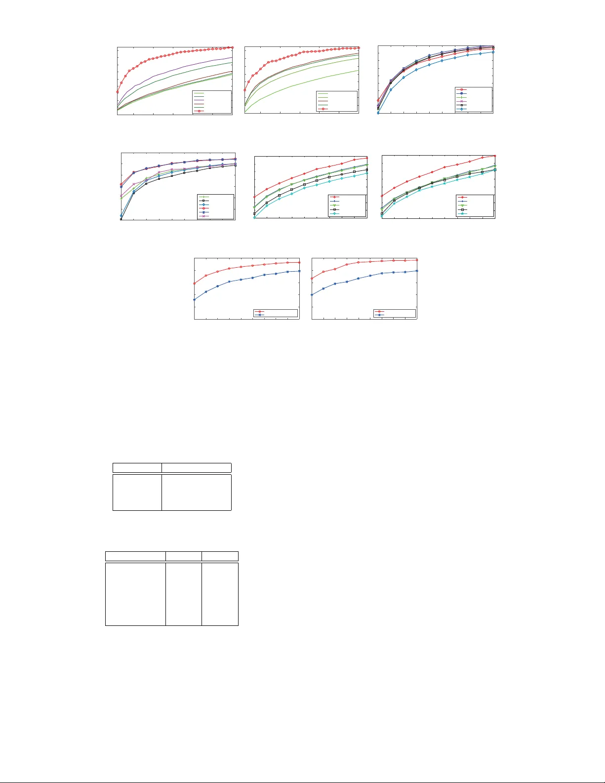
IEEE TRANSACTIONS ON P A TTERN ANAL YSIS AND MACHINE INTELLIGENCE 1 Cross-Domain Visual Matching via Generaliz ed Similar ity Measure and F eature Lear ning Liang Lin, Guangrun W ang, W angmeng Zuo , Xiangchu F eng, and Lei Zhang Abstract —Cross-domain visual data matching is one of the fundamental problems in man y real-world vision tasks, e.g., matching persons across ID photos and surveillance videos. Conv entional approaches to this problem usually in volv es two steps: i) projecting samples from different domains into a common space , and ii) computing (dis-)similarity in this space based on a cer tain distance. In this paper , we present a nov el pairwise similarity measure that advances e xisting models by i) e xpanding traditional linear projections into afﬁne transf or mations and ii) fusing afﬁne Mahalanobis distance and Cosine similarity by a data-driven combination. Moreo ver , we unify our similarity measure with feature representation learning via deep conv olutional neural networks. Speciﬁcally , we incor porate the similarity measure matrix into the deep architecture, enabling an end-to-end wa y of model optimization. W e extensiv ely ev aluate our generalized similarity model in se veral challenging cross-domain matching tasks: person re-identiﬁcation under diff erent views and face v eriﬁcation ov er different modalities (i.e., f aces from still images and videos, older and y ounger faces , and sketch and photo por traits). The e xperimental results demonstrate superior performance of our model over other state-of-the-art methods. Index T erms —Similar ity model, Cross-domain matching, P erson v eriﬁcation, Deep lear ning. F 1 I N T R O D U C T I O N V I S U A L similarity matching is arguably consider ed as one of the most fundamental problems in computer vision and pattern recognition, and this pr oblem becomes more challenging when dealing with cross-domain data. For example, in still-video face retrieval, a newly rising task in visual surveillance, faces from still images captured under a constrained environment ar e utilized as the queries to ﬁnd the matches of the same identity in unconstrained videos. Age-invariant and sketch-photo face veriﬁcation tasks are also examples of cross-domain image matching. Some ex- amples in these applications are shown in Figure 1. Conventional approaches (e.g., canonical corr elation analysis [1] and partial least square regression [2]) for cross- domain matching usually follow a procedure of two steps: 1) Samples from different modalities are ﬁrst projected into a common space by learning a transformation. One may simplify the computation by assuming that these cross domain samples share the same projection. 2) A certain distance is then utilized for measuring the similarity/disimilarity in the pr ojection space. Usually Euclidean distance or inner product are used. Suppose that x and y are two samples of differ ent modalities, and U and V are two projection matrices ap- plied on x and y , respectively . Ux and Vy are usually formulated as linear similarity transformations mainly for • L. Lin and G. Wang are with School of Data and Computer Science, Sun Y at-sen University , Guangzhou, P . R. China. Email: linliang@ieee.org; wanggrun@mail2.sysu.edu.cn. • W . Zuo is with School of Computer Science and T echnology, Harbin Institute of T echnology, Harbin, P . R. China. Email: cswmzuo@gmail.com. • X. Feng is with School of Math. and Statistics, Xidian University, Xi’an, P . R. China. Email: xcfeng@mail.xidian.edu.cn. • L. Zhang is with Dept. of Computing, The Hong Kong Polytechnic University , Hong Kong. Email: cslzhang@comp.polyu.edu.hk. (a) (b) (c) (d) Fig. 1: T ypical examples of matching cross-domain visual data. (a) Faces from still images and vidoes. (b) Front- and side-view persons. (c) Older and younger faces. (d) Photo and sketch faces. the convenience of optimization. A similarity transforma- tion has a good property of preserving the shape of an object that goes through this transformation, but it is limited in capturing complex deformations that usually exist in various real problems, e.g., translation, shearing, and their compositions. On the other hand, Mahalanobis distance, Cosine similarity , and their combination have been widely IEEE TRANSACTIONS ON P A TTERN ANAL YSIS AND MACHINE INTELLIGENCE 2 studied in the research of similarity metric learning, but it remains less investigated on how to unify feature learning and similarity learning, in particular , how to combine Ma- halanobis distance with Cosine similarity and integrate the distance metric with deep neural networks for end-to-end learning. T o address the above issues, in this work we pr esent a more general similarity measure and unify it with deep convolutional representation learning. One of the key inno- vations is that we generalize the existing similarity models from two aspects. First, we extend the similarity transforma- tions Ux and Vy to the afﬁne transformations by adding a translation vector into them, i.e., replacing Ux and Vy with L A x + a and L B y + b , respectively . Afﬁne transformation is a generalization of similarity transformation without the requir ement of pr eserving the original point in a linear space, and it is able to capture more complex deforma- tions. Second, unlike the traditional approaches choosing either Mahalanobis distance or Cosine similarity , we com- bine these two measures under the afﬁne transformation. This combination is realized in a data-driven fashion, as discussed in the Appendix, resulting in a novel generalized similarity measure, deﬁned as: S ( x , y ) = [ x T y T 1]   A C d C T B e d T e T f     x y 1   , (1) where sub-matrices A and B are positive semi-deﬁnite, repr esenting the self-corr elations of the samples in their own domains, and C is a correlation matrix cr ossing the two domains. Figure 2 intuitively explains the idea 1 . In this example, it is observed that Euclidean distance under the linear trans- formation, as (a) illustrates, can be regar ded as a special case of our model with A = U T U , B = V T V , C = − U T V , d = 0 , e = 0 , and f = 0 . Our similarity model can be viewed as a generalization of several recent metric learning models [3] [4]. Experimental results validate that the intro- duction of ( d , e , f ) and more ﬂexible setting on ( A , B , C ) do improve the matching performance signiﬁcantly . Another innovation of this work is that we unify feature repr esentation learning and similarity measure learning. In literature, most of the existing models are performed in the original data space or in a pre-deﬁned feature space, that is, the feature extraction and the similarity measur e are studied separately . These methods may have several drawbacks in practice. For example, the similarity models heavily rely on feature engineering and thus lack of gen- erality when handling problems under different scenarios. Moreover , the interaction between the feature repr esen- tations and similarity measures is ignored or simpliﬁed, thus limiting their performances. Meanwhile, deep learning, especially the Convolutional Neural Network (CNN), has demonstrated its effectiveness on learning discriminative features from raw data and beneﬁted to build end-to-end learning frameworks. Motivated by these works, we build 1. Figure 2 does not imply that our model geometrically aligns two samples to be matched. Using this example we emphasize the superi- ority of the afﬁne transformation over the traditional linear similarity transformation on capturing pattern variations in the feature space. (a) (b) Fig. 2: Illustration of the generalized similarity model. Con- ventional appr oaches pr oject data by simply using the linear similarity transformations (i.e., U and V ), as illustrated in (a), where Euclidean distance is applied as the distance metric. As illustrated in (b), we improve existing models by i) expanding the traditional linear similarity transformation into an af ﬁne transformation and ii) fusing Mahalanobis distance and Cosine similarity . One can see that the case in (a) is a simpliﬁed version of our model. Please refer to Appendix section for the deduction details. a deep architectur e to integrate our similarity measure with the CNN-based feature representation learning. Our archi- tecture takes raw images of differ ent modalities as the inputs and automatically produce their representations by sequen- tially stacking shared sub-network upon domain-speciﬁc subnetworks. Upon these layers, we further incorporate the components of our similarity measure by stimulating them with several appended structured neural network layers. The feature learning and the similarity model learning are thus integrated for end-to-end optimization. In sum, this paper makes three main contributions to cross-domain similarity measure learning. • First, it presents a generic similarity measure by general- izing the traditional linear projection and distance metrics into a uniﬁed formulation. Our model can be viewed as a generalization of several existing similarity learning models. • Second, it integrates feature learning and similarity mea- sure learning by building an end-to-end deep architecture of neural networks. Our deep architectur e effectively im- proves the adaptability of learning with data of differ ent modalities. • Third, we extensively evaluate our framework on four challenging tasks of cross-domain visual matching: per- son re-identiﬁcation across views 2 , and face veriﬁcation under dif ferent modalities (i.e., faces from still images and videos, older and younger faces, and sketch and photo portraits). The experimental results show that our similar- ity model outperforms other state-of-the-arts in three of 2. Person re-identiﬁcation is arguably a cross-domain matching prob- lem. W e introduce it in our experiments since this problem has been receiving increasing attentions recently . IEEE TRANSACTIONS ON P A TTERN ANAL YSIS AND MACHINE INTELLIGENCE 3 the four tasks and achieves the second best performance in the other one. The rest of the paper is organized as follows. Section 2 reviews related work. Section 3 introduces our generalized similarity model and discusses its connections to existing works. Section 4 presents the pr oposed deep neural network architectur e and the learning algorithm in Section 4.2. The experimental results, comparisons and ablation studies are presented in Section 5. Section 6 concludes the paper . 2 R E L A T E D W O R K In literatur e, to cope with the cr oss-domain matching of visual data, one can learn a common space for different domains. CCA [1] learns the common space via maximizing cross-view correlation, while PLS [2] is learned via maximiz- ing cross-view covariance. Coupled information-theoretic encoding is proposed to maximize the mutual information [5]. Another conventional strategy is to synthesize samples from the input domain into the other domain. Rather than learning the mapping between two domains in the data space, dictionary learning [6] [7] can be used to alleviate cross-domain heterogeneity , and semi-coupled dictionary learning (SCDL [7]) is proposed to model the relationship on the sparse coding vectors fr om the two domains. Duan et al. proposed another framework called domain adaptation machine (DAM) [8] for multiple source domain adaption but they need a set of pre-trained base classiﬁers. V arious discriminative common space approaches have been developed by utilizing the label information. Super- vised information can be employed by the Rayleigh quotient [1], tr eating the label as the common space [9], or employing the max-margin rule [10]. Using the SCDL framework, struc- tured group sparsity was adopted to utilize the label infor- mation [6]. Generalization of discriminative common space to multiview was also studied [11]. Kan et al. proposed a multiview discriminant analysis (MvDA [12]) method to obtain a common space for multiple views by optimizing both inter-view and intra-view Rayleigh quotient. In [13], a method to learn shape models using local curve segments with multiple types of distance metrics was proposed. Moreover , for most existing multiview analysis methods, the target is deﬁned based on the standard inner product or distance between the samples in the feature space. In the ﬁeld of metric learning, several generalized similarity / distance measures have been studied to impr ove r ecognition performance. In [4] [14], the generalized distance / simi- larity measures are formulated as the dif ference between the distance component and the similarity component to take into account both cross inner product term and two norm terms. Li et al. [3] adopted the second-order decision function as distance measure without considering the pos- itive semi-deﬁnite (PSD) constraint. Chang and Y eung [15] suggested an approach to learn locally smooth metrics using local af ﬁne transformations while preserving the topological structure of the original data. These distance / similarity measures, however , were developed for matching samples from the same domain, and they cannot be directly applied to cross domain data matching. T o extend traditional single-domain metric learning, Mignon and Jurie [16] suggested a cr oss-modal metric learn- ing (CMML) model, which learns domain-speciﬁc transfor- mations based on a generalized logistic loss. Zhai et al. [17] incorporated the joint graph regularization with the heterogeneous metric learning model to improve the cross- media retrieval accuracy . In [16], [17], Euclidean distance is adopted to measure the dissimilarity in the latent space. In- stead of explicitly learning domain-speciﬁc transformations, Kang et al. [18] learned a low rank matrix to parameterize the cross-modal similarity measure by the accelerated prox- imal gradient (APG) algorithm. However , these methods are mainly based on the common similarity or distance measures and none of them addresses the feature learning problem under the cross-domain scenarios. Instead of using hand-crafted features, learning feature repr esentations and contextual relations with deep neu- ral networks, especially the convolutional neural network (CNN) [19], has shown great potential in various pattern recognition tasks such as object recognition [20] and seman- tic segmentation [21]. Signiﬁcant performance gains have also been achieved in face recognition [22] and person re- identiﬁcation [23] [24] [25] [26], mainly attributed to the progr ess in deep learning. Recently , several deep CNN- based models have been explored for similarity matching and learning. For example, Andrew et al. [27] proposed a multi-layer CCA model consisting of several stacked non- linear transformations. Li et al. [28] learned ﬁlter pairs via deep networks to handle misalignment, photometric and geometric transforms, and achieved promising results for the person re-identiﬁcation task. W ang et al. [29] learned ﬁne-grained image similarity with deep ranking model. Y i et al. [30] presented a deep metric learning approach by generalizing the Siamese CNN. Ahmed et al. [25] proposed a deep convolutional architecture to measure the similarity between a pair of pedestrian images. Besides the shared convolutional layers, their network also includes a neigh- borhood differ ence layer and a patch summary layer to compute cross-input neighborhood differ ences. Chen et al. [26] proposed a deep ranking framework to learn the joint repr esentation of an image pair and return the similarity score directly , in which the similarity model is replaced by full connection layers. Our deep model is partially motivated by the above works, and we target on a more powerful solution of cross- domain visual matching by incorporating a generalized similarity function into deep neural networks. Moreover , our network architectur e is differ ent from existing works, leading to new state-of-the-art results on several challenging person veriﬁcation and recognition tasks. 3 G E N E R A L I Z E D S I M I L A R I T Y M O D E L In this section, we ﬁrst intr oduce the formulation of our deep generalized similarity model and then discuss the con- nections between our model and existing similarity learning methods. 3.1 Model Form ulation According to the discussion in Section 1, our generalized similarity measure extends the traditional linear projection and integrates Mahalanobis distance and Cosine similarity IEEE TRANSACTIONS ON P A TTERN ANAL YSIS AND MACHINE INTELLIGENCE 4 into a generic form, as shown in Eqn. (1). As we derive in the Appendix, A and B in our similarity measure are positive semi-deﬁnite but C does not obey this constraint. Hence, we can further factorize A , B and C , as: A = L A T L A , B = L B T L B , C = − L x C T L y C . (2) Moreover , our model extracts featur e r epresentation (i.e., f 1 ( x ) and f 2 ( y ) ) from the raw input data by utilizing the CNNs. Incorporating the feature representation and the above matrix factorization into Eqn. (1), we can thus have the following similarity model: ˜ S ( x , y ) = S ( f 1 ( x ) , f 2 ( y )) (3) = [ f 1 ( x ) T f 2 ( y ) T 1]   A C d C T B e d T e T f     f 1 ( x ) f 2 ( y ) 1   = k L A f 1 ( x ) k 2 + k L B f 2 ( y ) k 2 + 2 d T f 1 ( x ) − 2( L x C f 1 ( x )) T ( L y C f 2 ( y )) + 2 e T f 2 ( y ) + f . Speciﬁcally , L A f 1 ( x ) , L x C f 1 ( x ) , d T f 1 ( x ) can be regarded as the similarity components for x , while L B f 2 ( y ) , L y C f 2 ( y ) , d T f 2 ( y ) accordingly for y . These similarity components are modeled as the weights that connect neurons of the last two layers. For example, a portion of output activations repre- sents L A f 1 ( x ) by taking f 1 ( x ) as the input and multiplying the corresponding weights L A . In the following, we discuss the formulation of our similarity learning. The objective of our similarity learning is to seek a function ˜ S ( x , y ) that satisﬁes a set of similarity/disimilarity constraints. Instead of learning similarity function on hand- crafted feature space, we take the raw data as input, and introduce a deep similarity learning framework to integrate nonlinear feature learning and generalized similarity learn- ing. Recall that our deep generalized similarity model is in Eqn. (1). ( f 1 ( x ) , f 2 ( y )) are the feature representations for samples of differ ent modalities, and we use W to indicate their parameters. W e denote Φ = ( L A , L B , L x C , L y C , d , e , f ) as the similarity components for sample matching. Note that ˜ S ( x , y ) is asymmetric, i.e., ˜ S ( x , y ) 6 = ˜ S ( y , x ) . This is rea- sonable for cross-domain matching, because the similarity components are domain-speciﬁc. Assume that D = { ( { x i , y i } , ` i ) } N i =1 is a training set of cross-domain sample pairs, where { x i , y i } denotes the i th pair , and ` i denotes the corresponding label of { x i , y i } indicating whether x i and y i are from the same class: ` i = ` ( x i , y i ) =  − 1 , c ( x ) = c ( y ) 1 , otherwise , (4) where c ( x ) denotes the class label of the sample x . An ideal deep similarity model is expected to satisfy the following constraints: ˜ S ( x i , y i )  < − 1 , if ` i = − 1 ≥ 1 , otherwise (5) for any { x i , y i } . Note that the feasible solution that satisﬁes the above constraints may not exist. T o avoid this scenario, we relax the hard constraints in Eqn. (5) by introducing a hinge-like loss: G ( W , Φ ) = N X i =1 (1 − ` i ˜ S ( x i , y i )) + . (6) T o improve the stability of the solution, some regularizers are further introduced, resulting in our deep similarity learning model: ( ˆ W , ˆ Φ ) = arg min W , Φ N X i =1 (1 − ` i ˜ S ( x i , y i )) + + Ψ( W , Φ ) , (7) where Ψ( W , Φ ) = λ k W k 2 + µ k Φ k 2 denotes the r egularizer on the parameters of the feature representation and gener- alized similarity models. 3.2 Connection with Existing Models Our generalized similarity learning model is a generaliza- tion of many existing metric learning models, while they can be treated as special cases of our model by imposing some extra constraints on ( A , B , C , d , e , f ) . Conventional similarity model usually is deﬁned as S M ( x , y ) = x T My , and this form is equivalent to our model, when A = B = 0 , C = 1 2 M , d = e = 0 , and f = 0 . Similarly , the Mahalanobis distance D M ( x , y ) = ( x − y ) T M ( x − y ) is also regarded as a special case of our model, when A = B = M , C = − M , d = e = 0 , and f = 0 . In the following, we connect our similarity model to two state-of-the-art similarity learning methods, i.e., LADF [3] and Joint Bayesian [4]. In [3], Li et al. pr oposed to learn a decision func- tion that jointly models a distance metric and a locally adaptive thr esholding rule, and the so-called LADF (i.e., Locally-Adaptive Decision Function) is formulated as a second-order large-margin regularization problem. Specif- ically , LADF is deﬁned as: F ( x , y ) = x T Ax + y T Ay + 2 x T Cy + d T ( x + y ) + f . (8) One can observe that F ( x , y ) = S ( x , y ) when we set B = A and e = d in our model. It should be noted that LADF treats x and y using the same metrics, i.e., A for both x T Ax and y T Ay , and d for d T x and d T y . Such a model is reasonable for matching samples with the same modality , but may be unsuitable for cross-domain matching where x and y are with different modalities. Compared with LADF , our model uses A and d to calculate x T Ax and d T x , and uses B and e to calculate y T By and e T y , making our model more effective for cross- domain matching. In [4], Chen et al. extended the classical Bayesian face model by learning a joint distributions (i.e., intra-person and extra-person variations) of sample pairs. Their decision function is posed as the following form: J ( x , y ) = x T Ax + y T Ay − 2x T Gy . (9) Note that the similarity metric model proposed in [14] also adopted such a form. Interestingly , this decision function is also a special variant of our model by setting B = A , C = − G , d = 0 , e = 0 , and f = 0 . IEEE TRANSACTIONS ON P A TTERN ANAL YSIS AND MACHINE INTELLIGENCE 5 200 ×3×180×130 20 ×3×180×130 5×5 Conv + ReLU + 3×3 MaxPool 5×5 Conv + ReLU + 3×3 MaxPool FC FC f 2 (y y ) f 1 (x x ) L B f 2 (y y ) L C f 2 (y y ) e T f 2 (y y ) y L A f 1 (x x ) L C f 1 (x x ) d T f 1 (x x ) x 200 ×32×30×21 220 ×32×9×6 220 ×400 x y Concate Slice 20 ×801 200 ×801 Domain-specific sub-network Similarity sub-network g 1 (x x ) g 2 (y y ) 5×5 Conv + ReLU + 3×3 MaxPool 220 ×400 200 ×400 20 ×400 FC FC 20 ×32×30×21 Shared sub-network Fig. 3: Deep ar chitecture of our similarity model. This ar chitecture is comprised of thr ee parts: domain-speciﬁc sub-network, shared sub-network and similarity sub-network. The ﬁrst two parts extract feature representations from samples of differ ent domains, which are built upon a number of convolutional layers, max-pooling operations and fully-connected layers. The similarity sub-network includes two structured fully-connected layers that incorporate the similarity components in Eqn. (3). In summary , our similarity model can be regar ded as the generalization of many existing cross-domain matching and metric learning models, and it is more ﬂexible and suitable for cross-domain visual data matching. 4 J O I N T S I M I L A R I T Y A N D F E AT U R E L E A R N I N G In this section, we introduce our deep architectur e that integrates the generalized similarity measure with convo- lutional feature representation learning. 4.1 Deep Ar chitecture As discussed above, our model deﬁned in Eqn. (7) jointly handles similarity function learning and feature learning. This integration is achieved by building a deep architecture of convolutional neural networks, which is illustrated in Figure 3. It is worth mentioning that our architecture is able to handle the input samples of dif ferent modalities with unequal numbers, e.g., 20 samples of x and 200 samples of y are fed into the network in a way of batch processing. From left to right in Figure 3, two domain-speciﬁc sub- networks g 1 ( x ) and g 2 ( y ) are applied to the samples of two dif ferent modalities, respectively . Then, the outputs of g 1 ( x ) and g 2 ( y ) are concatenated into a shared sub- network f ( · ) . W e make a superposition of g 1 ( x ) and g 2 ( y ) to feed f ( · ) . At the output of f ( · ) , the featur e repr esentations of the two samples are extracted separately as f 1 ( x ) and f 2 ( y ) , which is indicated by the slice operator in Figure 3. Finally , these learned feature representations are utilized in the structured fully-connected layers that incorporate the similarity components deﬁned in Eqn. (3). In the following, we introduce the detailed setting of the three sub-networks. Domain-speciﬁc sub-network. W e separate two branches of neural networks to handle the samples from differ ent domains. Each network branch includes one convolutional layer with 3 ﬁlters of size 5 × 5 and the stride step of 2 pixels. The rectiﬁed nonlinear activation is utilized. Then, we follow by a one max-pooling operation with size of 3 × 3 and its stride step is set as 3 pixels. Shared sub-network. For this component, we stack one convolutional layer and two fully-connected layers. The convolutional layer contains 32 ﬁlters of size 5 × 5 and the ﬁlter stride step is set as 1 pixel. The kernel size of the max- pooling operation is 3 × 3 and its stride step is 3 pixels. The output vectors of the two fully-connected layers are of 400 dimensions. W e further normalize the output of the second fully-connected layer before it is fed to the next sub- network. Similarity sub-network. A slice operator is ﬁrst applied in this sub-network, which partitions the vectors into two groups corresponding to the two domains. For the example in Figure 3, 220 vectors are grouped into two sets, i.e., f 1 ( x ) and f 2 ( y ) , with size of 20 and 200 , respectively . f 1 ( x ) and f 2 ( y ) ar e both of 400 dimensions. Then, f 1 ( x ) and f 2 ( y ) are fed to two branches of neural network, and each branch includes a fully-connected layer . W e divide the activations of these two layers into six parts according to the six similarity components. As is shown in Figure 3, in the top branch the neural layer connects to f 1 ( x ) and outputs L A f 1 ( x ) , L x C f 1 ( x ) , and d T f 1 ( x ) , respectively . In the bottom branch, the layer outputs L B f 2 ( y ) , L y C f 2 ( y ) , and e T f 2 ( y ) , respectively , by connecting to f 2 ( y ) . In this way , the similarity measure is tightly integrated with the feature repr esentations, and they can be jointly optimized during the model training. Note that f is a parameter of the gen- eralized similarity measure in Eqn. (1). Experiments show that the value of f only affects the learning convergence rather than the matching performance. Thus we empirically set f = − 1 . 9 in our experiments. In the deep architecture, we can observe that the similar- ity components of x and those of y do not interact to each other by the factorization until the ﬁnal aggr egation calcula- tion, that is, computing the components of x is independent of y . This leads to a good property of efﬁcient matching. In particular , for each sample stored in a database, we can pre- computed its feature representation and the corresponding similarity components, and the similarity matching in the testing stage will be very fast. IEEE TRANSACTIONS ON P A TTERN ANAL YSIS AND MACHINE INTELLIGENCE 6 4.2 Model T raining In this section, we discuss the learning method for our similarity model training. T o avoid loading all images into memory , we use the mini-batch learning approach, that is, in each training iteration, a subset of the image pairs are fed into the neural network for model optimization. For notation simplicity in discussing the learning algo- rithm, we start by introducing the following deﬁnitions: ˜ x ∆ = [ L A f 1 ( x ) L x C f 1 ( x ) d T f 1 ( x ) ] T ˜ y ∆ = [ L B f 2 ( y ) L y C f 2 ( y ) e T f 2 ( y ) ] T , (10) where ˜ x and ˜ y denote the output layer ’s activations of the samples x and y . Prior to incorporating Eqn. (10) into the similarity model in Eqn. (3), we introduce three transforma- tion matrices (using Matlab representation): P 1 =  I r × r 0 r × ( r +1)  , P 2 =  0 r × r I r × r 0 r × 1  , p 3 =  0 1 × 2 r 1 1 × 1  T , (11) where r equals to the dimension of the output of shared neural network (i.e., the dimension of f ( x ) and f ( y ) ), an I indicates the identity matrix. Then, our similarity model can be re-written as: ˜ S ( x , y ) = ( P 1 ˜ x ) T P 1 ˜ x + ( P 1 ˜ y ) T P 1 ˜ y − 2( P 2 ˜ x ) T P 2 ˜ y +2 p T 3 ˜ x + 2 p T 3 ˜ y + f . (12) Incorporating Eqn. (12) into the loss function Eqn. (6), we have the following objective: G ( W , Φ ; D ) = N P i =1 { 1 − ` i [ ( P 1 e x i ) T P 1 e x i + ( P 1 e y i ) T P 1 e y i − 2( P 2 e x i ) T P 2 e y i + 2 p T 3 e x i + 2 p T 3 e y i + f ] } + , (13) where the summation term denotes the hinge-like loss for the cr oss domain sample pair { ˜ x i , ˜ y i } , N is the total number of pairs, W repr esents the feature repr esentation of differ ent domains and Φ repr esents the similarity model. W and Φ are both embedded as weights connecting neurons of layers in our deep neural network model, as Figure 3 illustrates. The objective function in Eqn. (13) is deﬁned in sample- pair-based form. T o optimize it using SGD, one should ap- ply a certain scheme to generate mini-batches of the sample pairs, which usually costs much computation and memory . Note that the sample pairs in training set D are constructed from the original set of samples from different modalities Z = {{X } , {Y }} , wher e X = { x 1 , ..., x j , ..., x M x } and Y = { y 1 , ..., y j , ..., y M y } . The superscript denotes the sam- ple index in the original training set, e.g., x j ∈ X = { x 1 , ..., x j , ..., x M x } and y j ∈ Y = { y 1 , ..., y j , ..., y M y } , while the subscript denotes the index of sample pairs, e.g., x i ∈ { x i , y i } ∈ D . M x and M y denote the total number of samples from differ ent domains. W ithout loss of generality , we deﬁne z j = x j and z M x + j = y j . For each pair { x i , y i } in D , we have z j i, 1 = x i and z j i, 2 = y i with 1 ≤ j i, 1 ≤ M x and M x + 1 ≤ j i, 2 ≤ M z (= M x + M y ) . And we also have e z j i, 1 = e x i and e z j i, 2 = e y i . Therefor e, we rewrite Eqn. (13) in a sample-based form: L ( W , Φ ; Z ) = N P i =1 { 1 − ` i [ ( P 1 e z j i, 1 ) T P 1 e z j i, 1 + ( P 1 e z j i, 2 ) T P 1 e z j i, 2 − 2( P 2 e z j i, 1 ) T P 2 e z j i, 2 + 2 p T 3 e z j i, 1 + 2 p T 3 e z j i, 2 + f ] } + , (14) Given Ω = ( W , Φ ) , the loss function in Eqn. (7) can also be rewritten in the sample-based form: H ( Ω ) = L ( Ω ; Z ) + Ψ( Ω ) . (15) The objective in Eqn. (15) can be optimized by the mini- batch back propagation algorithm. Speciﬁcally , we update the parameters by gradient descent: Ω = Ω − α ∂ ∂ Ω H ( Ω ) , (16) where α denotes the learning rate. The key problem of solving the above equation is calculating ∂ ∂ Ω L ( Ω ) . As is discussed in [31], there are two ways to this end, i.e., pair- based gradient descent and sample-based gradient descent. Here we adopt the latter to reduce the requir ements on computation and memory cost. Suppose a mini-batch of training samples { z j 1 , x , ..., z j n x , x , z j 1 , y , ..., z j n y , y } fr om the original set Z , where 1 ≤ j i, x ≤ M x and M x + 1 ≤ j i, y ≤ M z . Following the chain rule, calculating the gradient for all pairs of samples is equivalent to summing up the gradient for each sample, ∂ ∂ Ω L ( Ω ) = X j ∂ L ∂ ˜ z j ∂ ˜ z j ∂ Ω , (17) where j can be either j i, x or j i, y . Using z j i, x as an example, we ﬁrst intr oduce an in- dicator function 1 z j i, x ( z j i, y ) before calculating the partial derivative of output layer activation for each sample ∂ L ∂ ˜ z j i, x . Speciﬁcally , we deﬁne 1 z j i, x ( z j i, y ) = 1 when { z j i, x , z j i, y } is a sample pair and ` j i, x ,j i, y ˜ S ( z j i, x , z j i, y ) < 1 . Otherwise we let 1 z j i, x ( z j i, y ) = 0 . ` j i, x ,j i, y , indicating where z j i, x and z j i, y are from the same class. W ith 1 z j i, x ( z j i, y ) , the gradient of ˜ z j i, x can be written as ∂ L ∂ ˜ z j i, x = − X j i, y 2 1 z j i, x ( z j i, y ) ` j i, x ,j i, y ( P T 1 P 1 ˜ z j i, x − P T 2 P 2 ˜ z j i, y + p 3 ) . (18) The calculation of ∂ L ∂ ˜ z j i, y can be conducted in a similar way . The algorithm of calculating the partial derivative of output layer activation for each sample is shown in Algorithm 1. Note that all the three sub-networks in our deep ar- chitecture are differentiable. W e can easily use the back- propagation procedur e [19] to compute the partial deriva- tives with respect to the hidden layers and model pa- rameters Ω . W e summarize the overall procedure of deep generalized similarity measure learning in Algorithm 2. If all the possible pairs are used in training, the sample- based form allows us to generate n x × n y sample pairs from a mini-batch of n x + n y . On the other hand, the sample-pair-based form may require 2 n x n y samples or less to generate n x × n y sample pairs. In gradient compu- tation, from Eqn. (18), for each sample we only require calculating P T 1 P 1 ˜ z j i, x once and P T 2 P 2 ˜ z j i, y n y times in the sample-based form. While in the sample-pair-based form, P T 1 P 1 ˜ z j i, x and P T 2 P 2 ˜ z j i, y should be computed n x and n y IEEE TRANSACTIONS ON P A TTERN ANAL YSIS AND MACHINE INTELLIGENCE 7 Algorithm 1 Calculate the derivative of the output layer ’s activation for each sample Input: The output layer ’s activation for all samples Output: The partial derivatives of output layer ’s activation for all the samples 1: for each sample z j do 2: Initialize the partner set M j containing the sample z j with M j = ∅ ; 3: for each pair { x i , y i } do 4: if pair { x i , y i } contains the sample z j then 5: if pair { x i , y i } satisﬁes ` i ˜ S ( x i , y i ) < 1 then 6: M i ← {M i , the corr esponding partner of z j in { x i , y i }} ; 7: end if 8: end if 9: end for 10: Compute the derivatives for the sample z j with all the partners in M j , and sum these derivatives to be the desired partial derivative for sample z j ’s output layer ’s activation using Eqn. (18); 11: end for times, r espectively . In sum, the sample-based form generally results in less computation and memory cost. Algorithm 2 Generalized Similarity Learning Input: T raining set, initialized parameters W and Φ , learning rate α , t ← 0 Output: Network parameters W and Φ 1: while t < = T do 2: Sample training pairs D ; 3: Feed the sampled images into the network; 4: Perform a feed-forward pass for all the samples and compute the net activations for each sample z i ; 5: Compute the partial derivative of the output layer ’s activation for each sample by Algorithm 1. 6: Compute the partial derivatives of the hidden layers’ activations for each sample following the chain rule; 7: Compute the desired gradients ∂ ∂ Ω H ( Ω ) using the back-propagation procedure; 8: Update the parameters using Eqn. (16); 9: end while Batch Process Implementation. Suppose that the train- ing image set is divided into K categories, each of which contains O 1 images from the ﬁrst domain and O 2 images from the second domain. Thus we can obtain a maximum number ( K × O 1 ) × ( K × O 2 ) of pairwise samples, which is quadratically more than the number of source images K × ( O 1 + O 2 ) . In real application, since the number of stored images may reach millions, it is impossible to load all the data for network training. T o overcome this problem, we implement our learning algorithm in a batch-process manner . Speciﬁcally , in each iteration, only a small subset of cross domain image pairs are generated and fed to the network for training. According to our massive ex- periments, randomly generating image pairs is infeasible, which may cause the image distribution over the special batch becoming scattered, making valid training samples for a certain category very few and degenerating the model. Besides, images in any pair are almost impossible to come from the same class, making the positive samples very few . In order to overcome this problem, an effective cross domain image pair generation scheme is adopted to train our generalized similarity model. For each round, we ﬁrst randomly choose b K instance categories. For each category , a number of c O 1 images ﬁrst domain and a number of c O 2 from second domain ar e randomly selected. For each selected images in ﬁrst domain, we randomly take samples from the second domain and the proportions of positive and negative samples are equal. In this way , images distributed over the generated samples are relatively centralized and the model will effectively converge. 5 E X P E R I M E N T S In this section, we apply our similarity model in four rep- resentative tasks of matching cross-domain visual data and adopt several benchmark datasets for evaluation: i) person re-identiﬁcation under different views on CUHK03 [28] and CUHK01 [32] datasets; ii) age-invariant face recognition on MORPH [33], CACD [34] and CACD-VS [35] datasets; iii) sketch-to-photo face matching on CUFS dataset [36]; iv) face veriﬁcation over still-video domains on COX face dataset [37]. On all these tasks, state-of-the-art methods are employed to compare with our model. Experimental setting. Mini-batch learning is adopted in our experiments to save memory cost. In each task, we randomly select a batch of sample from the original training set to generate a number of pairs (e.g., 4800 ). The initial parameters of the convolutional and the full connection layers are set by two zero-mean Gaussian Distributions, whose standard deviations are 0 . 01 and 0 . 001 respectively . Other speciﬁc settings to different tasks are included in the following sub-sections. In addition, ablation studies are presented to reveal the beneﬁt of each main component of our method, e.g., the generalized similarity measure and the joint optimization of CNN feature repr esentation and metric model. W e also implement several variants of our method by simplifying the similarity measures for comparison. 5.1 P erson Re-identiﬁcation Person re-identiﬁcation, aiming at matching pedestrian im- ages across multiple non-overlapped cameras, has attracted increasing attentions in surveillance. Despite that consider- able efforts have been made, it is still an open problem due to the dramatic variations caused by viewpoint and pose changes. T o evaluate this task, CUHK03 [28] dataset and CUHK01 [32] dataset are adopted in our experiments. CUHK03 dataset [28] is one of the largest databases for person re-identiﬁcation. It contains 14,096 images of 1,467 pedestrians collected fr om 5 dif ferent pairs of camera views. Each person is observed by two disjoint camera views and has an average of 4.8 images in each view . W e follow the IEEE TRANSACTIONS ON P A TTERN ANAL YSIS AND MACHINE INTELLIGENCE 8 rank 5 1 01 52 02 53 0 identification rate 0 0.2 0.4 0.6 0.8 1 5.64%Euclid 20.65%DFPNN 54.74%IDLA 5.53%ITML 14.17%KISSME 13.51%LDM 7.29%LMNN 10.42%RANK 5.6%SDALF 8.76%eSDC 22.0%DRSCH 32.7%KML 58.4%Ours (a) CUHK03 rank 5 1 01 52 02 53 0 identification rate 0 0.2 0.4 0.6 0.8 1 10.52%Euclid 27.87%FPNN 65.00%IDLA 17.10%ITML 29.40%KISSME 26.45%LDM 21.17%LMNN 20.61%RANK 9.9%SDALF 22.82%eSDC 34.30%LMLF 66.50%Ours (b) CUHK01 Fig. 4: CMC curves on (a) CUHK03 [28] dataset and (b) CUHK01 [32] for evaluating person re-identiﬁcation. Our method has superior performances over existing state-of- the-arts overall. standard setting of using CUHK03 to randomly partition this dataset for 10 times, and a training set (including 1,367 persons) and a testing set (including 100 persons) are obtained without overlap. CUHK01 dataset [32] contains 971 individuals, each having two samples from disjoint cameras. Following the setting in [28] [25], we partition this dataset into a training set and a testing set: 100 individuals for testing and the others for training. For evaluation on these two benchmarks, the testing set is further randomly divided into a gallery set of 100 images (i.e., one image per person) and a probe set (includ- ing images of individuals from different camera views in contrast to the gallery set) without overlap for 10 times. W e use Cumulative Matching Characteristic (CMC) [38] as the evaluation metric in this task. In our model training, all of the images are resized to 250 × 100 , and cropped to the size of 230 × 80 at the center with a small random perturbation. During every round of learning, 4800 pairs of samples are constructed by selecting 60 persons (or classes) and constructing 80 pairs for each person (class). For CUHK01, due to each individual only have two samples, the 80 pairs per individual will contain some duplicated pairs. Results on CUHK03. W e compare our approach with several state-of-the-art methods, which can be gr ouped into three categories. First, we adopt ﬁve distance metric learning methods based on ﬁxed feature r epresentation, i.e. the Information Theoretic Metric Learning (ITML) [5], the Local Distance Metric Learning (LDM) [39], the Large Margin Nearest Neighbors (LMNN) [40], the learning-to- rank method (RANK) [41], and the Kernel-based Metric Learning method (KML) [23]. Following their implementa- tion, the handcrafted featur es of dense color histograms and dense SIFT uniformly sampled from patches are adopted. Second, three methods specially designed for person re- identiﬁcation are employed in the experiments: SDALF [42], KISSME [43], and eSDC [44]. Moreover , several recently proposed deep learning methods, including DRSCH [45], DFPNN [28] and IDLA [25], are also compared with our approach. DRSCH [45] is a supervised hashing framework for integrating CNN feature and hash code learning, while DFPNN and IDLA have been introduced in Section 2. The results are reported in Fig. 4 (a). It is encouraging to see that our approach signiﬁcantly outperforms the com- peting methods (e.g., improving the state-of-the-art rank- 1 accuracy from 54.74% (IDLA [25]) to 58.39%). Among the competing methods, ITML [5], LDM [39], LMNN [40], RANK [41], KML [23], SDALF [42], KISSME [43], and eSDC [44] are all based on hand-crafted features. And the superi- ority of our approach against them should be attributed to the deployment of both deep CNN featur es and generalized similarity model. DRSCH [45], DFPNN [28] and IDLA [25] adopted CNN for feature repr esentation, but their matching metrics are deﬁned based on traditional linear transforma- tions. Results on CUHK01. Fig. 4 (b) shows the results of our method and the other competing approaches on CUHK01. In addition to those used on CUHK03, one mor e method, i.e. LMLF [24], is used in the comparison experiment. LMLF [24] learns mid-level ﬁlters from automatically discovered patch clusters. According to the quantitative results, our method achieves a new state-of-the-art with a rank-1 accuracy of 66.50%. 5.2 Age-in variant F ace Recognition Age invariant face recognition is to decide whether two images with different ages belong to the same identity . The key challenge is to handle the large intra-subject variations caused by aging process while distinguishing differ ent iden- tities. Other factors, such as illumination, pose, and expres- sion, make age invariant face recognition more difﬁcult. W e conduct the experiments using three datasets, i.e., MORPH [33], CACD [34], and CACD-VS [35]. MORPH [33] contains more than 55,000 face images of 13,000 individuals, whose ages range from 16 to 77. The average number of images per individual is 4. The training set consists of 20,000 face images from 10,000 subjects, with each subject having two images with the largest age gap. The test set is composed of a gallery set and a pr obe set fr om the remaining 3,000 subjects. The gallery set is composed of the youngest face images of each subject. The probe set is composed of the oldest face images of each subject. This experimental setting is the same with those adopted in [46] and [34]. CACD [34] is a large scale dataset released in 2014, which contains more than 160,000 images of 2,000 celebrities. W e adopt a subset of 580 individuals from the whole database in our experiment, in which we manually remove the noisy images. Among these 580 individuals, the labels of images from 200 individuals have been originally provided, and we annotate the rest of the data. CACD includes lar ge variations not only in pose, illumination, expression but also in ages. IEEE TRANSACTIONS ON P A TTERN ANAL YSIS AND MACHINE INTELLIGENCE 9 2004 − 2006 2007 − 2009 2010 − 2012 0.5 0.55 0.6 0.65 0.7 0.75 MAP HFA CARC Deepface Ours − 1 Ours − 2 Fig. 5: The retrieval performances on CACD dataset for age-invariant face recognition. Ours-1 and Ours-2 are our method, while the latter uses more training samples. T ABLE 1: Experimental results for age-invariant face recog- nition. (a) Recognition rates on the MORPH dataset. Method Recognition rate TDBN [48] 60% 3D Aging Model [50] 79.8% MFDA [49] 83.9% HF A [46] 91.1% CARC [34] 92.8% Ours 94.4% (b) V eriﬁcation accuracy on the CACD-VS dataset. Method veriﬁcation accuracy HD-LBP [51] 81.6% HF A [46] 84.4% CARC [34] 87.6% Deepface [52] 85.4% Ours 89.8% Based on CACD, a veriﬁcation subset called CACD-VS [35] is further developed, which contains 2,000 positive pairs and 2,000 negative pairs. The setting and testing protocol of CACD-VS are similar to the well-known LFW benchmark [47], except that CACD-VS contains much more samples for each person. All of the images ar e resized to 200 × 150 . For data augmentation, images ar e cr opped to the size of 180 × 130 at the center with a small random perturbation when feeding to the neural network. Sample-based mini-batch setting is adopted, and 4,800 pairs are constructed for each iteration. Results on MORPH. W e compare our method with sev- eral state-of-the-art methods, including topological dynamic Bayesian network (TDBN) [48], cross-age refer ence coding (CARC) [34], probabilistic hidden factor analysis (HF A) [46], multi-feature discriminant analysis (MFDA) [49] and 3D aging model [50]. The results are reported in T able 1(a). Thanks to the use of CNN representation and generalized similarity measure, our method achieves the recognition rate of 94.35%, and signiﬁcantly outperforms the competing methods. Results on CACD. On this dataset, the protocol is to retrieve face images of the same individual fr om gallery sets by using a probe set, where the age gap between probe face images and gallery face images is large. Following the ex- perimental setting in [34], we set up 4 gallery sets according to the years when the photos were taken: [2004 − 2006] , [2007 − 2009] , [2010 − 2012] , and [2013] . And we use the set of [2013] as the probe set to search for matches in the rest of three sets. W e introduce several state-of-the-art methods for comparison, including CARC [34], HF A [46] and one deep learning based method, Deepface [52]. The results of CARC [34] and HF A [46] are borrowed from their papers. The results of Deepface [52] and our approach (i.e., Ours- 1) are implemented based on the 200 originally annotated individuals, where 160 samples are used for model training. From the quantitative results r eported in Figure 5, our model achieves superior performances over the competing methods. Furthermore, we also r eport the result of our method (i.e., Ours-2) by using images of 500 individuals as training samples. One can see that, the performance of our model can be further improved by increasing training data. Results on CACD-VS. Following the setting in [35], we further evaluate our approach by conducting the general face veriﬁcation experiment. Speciﬁcally , for all of the com- peting methods, we train the models on CACD and test on CACD-VS, and the optimal threshold value for matching is obtained by exhaustive search. The results produced by our methods and the others (i.e., CARC [34], HF A [46], HD- LBP [51] and Deepface [52]) are reported in T able 1 (b). It is worth mentioning that our method improves the state-of- the-art recognition rate from 87.6% (by CARC [34] [52]) to 89.8%. Thanks to the introduction of generalized similarity measure our appr oach achieves higher veriﬁcation accuracy than Deepface. Note that an explicit face alignment was adopted in [52] before the CNN feature extraction, which is not in our framework. 5.3 Sketch-photo F ace V eriﬁcation Sketch-photo face veriﬁcation is an interesting yet challeng- ing task, which aims to verify whether a face photo and a drawing face sketch belong to the same individual. This task has an important application of assisting law enforcement, i.e., using face sketch to ﬁnd candidate face photos. It is however dif ﬁcult to match photos and sketches in two differ ent modalities. For example, hand-drawing may bring unpredictable face distortion and variation compared to the real photo, and face sketches often lack of details that can be important cues for preserving identity . W e evaluate our model on this task using the CUFS dataset [36]. There are 188 face photos in this dataset, in which 88 are selected for training and 100 for testing. Each face has a corresponding sketch that is drawn by the artist. All of these face photos are taken at frontal view with a normal lighting condition and neutral expression. All of the photos/sketches are resized to 250 × 200 , and cropped to the size of 230 × 180 at the center with a small random perturbation. 1200 pairs of photos and sketches (i.e., including 30 individuals with each having 40 pairs) are constructed for each iteration during the model training. In the testing stage, we use face photos to form the gallery set and treat sketches as the probes. W e employ several existing approaches for comparison: the eigenface transformation based method (ET) [53], the multi-scale Markov random ﬁeld based method (MRF) [36], and MRF+ [54] (i.e., the lighting and pose robust version of [36]). It is worth mentioning that all of these competing methods need to ﬁrst synthesize face sketches by photo- sketch transformation, and then measure the similarity be- tween the synthesized sketches and the candidate sketches, IEEE TRANSACTIONS ON P A TTERN ANAL YSIS AND MACHINE INTELLIGENCE 10 rank 5 1 01 52 02 53 0 identification rate 0 0.1 0.2 0.3 0.4 0.5 0.6 0.7 0.8 0.9 5.64%Euclid 5.53%ITML 13.51%LDM 7.29%LMNN 10.42%RANK 31.85%Generalized (a) sim.+hand.fea, CUHK03 rank 5 1 01 52 02 53 0 identification rate 0.1 0.2 0.3 0.4 0.5 0.6 0.7 0.8 0.9 10.52%Euclid 17.10%ITML 21.17%LMNN 20.61%RANK 39.50%Generalized (b) sim.+hand.fea, CUHK01 rank 123456789 1 0 identification rate 0.5 0.55 0.6 0.65 0.7 0.75 0.8 0.85 0.9 0.95 58.4% Ours 55.0%LADF 52.4%BFR 54.4%Linear 53.2%Baseline-1 50.0%Baseline-2 (c) sim.+deep.fea CUHK03 rank 123456789 1 0 identification rate 0.88 0.9 0.92 0.94 0.96 0.98 1 91.8%BFR 88.1%Baseline-1 88.8%Baseline-2 94.4%Ours 93.9%LADF 92.3%Linear (d) sim.+deep.fea, MORPH 1 2 3 4 5 6 7 8 9 10 0.2 0.25 0.3 0.35 0.4 0.45 0.5 0.55 rank identification rate 28.45%Ours 22.08%LADF 21.69%BFR 17.58%Baseline − 1 15.00%Baseline − 2 (e) sim.+deep.fea, COX-V2S 1 2 3 4 5 6 7 8 9 10 0.2 0.25 0.3 0.35 0.4 0.45 0.5 0.55 rank identification rate 29.02%Ours 21.59%LADF 20.65%BFR 17.92%Baseline − 1 16.48%Baseline − 2 (f) sim.+deep.fea, COX-S2V rank 123456789 1 0 identification rate 0 0.2 0.4 0.6 0.8 1 58.4% deep. fea+gen. sim. 31.9%hand.fea+gen.sim. (g) deep/hand fea, CUHK03 rank 123456789 1 0 identification rate 0 0.2 0.4 0.6 0.8 1 66.50%deep.fea+gen.sim 39.50%hand.fea+gen.sim (h) deep/hand fea, CUHK01 Fig. 6: Results of the ablation studies demonstrating the effectiveness of each main component of our framework. The CMC curve and recognition rate are used for evaluation. The results of differ ent similarity models are shown using the handcrafted features (in (a) and (b)) and using the deep features (in (c) - (f) ), respectively . (g) and (h) show the performances with / without the deep feature learning while keeping the same similarity model. T ABLE 2: Recognition rates on the CUFS dataset for sketch- photo face veriﬁcation. Method Recognition rate ET [53] 71.0% MRF [36] 96.0% MRF+ [54] 99.0% Ours 100.0% T ABLE 3: Recognition rates on the COX face dataset. Method V2S S2V PSD [55] 9.90% 11.64% PMD [56] 6.40% 6.10% P AHD [57] 4.70% 6.34% PCHD [58] 7.93% 8.89% PSDML [59] 12.14% 7.04% PSCL-EA [37] 30.33 % 28.39% Ours 28.45% 29.02% while our approach works in an end-to-end way . The quan- titative results are reported in T able 2. Our method achieves 100% recognition rate on this dataset. 5.4 Still-video F ace Recognition Matching person faces across still images and videos is a newly rising task in intelligent visual surveillance. In these applications, the still images (e.g., ID photos) are usually captured under a controlled environment while the faces in surveillance videos are acquired under complex scenarios (e.g., various lighting conditions, occlusions and low reso- lutions). For this task, a large-scale still-video face recognition dataset, namely COX face dataset, has been released r e- cently 3 , which is an extension of the COX-S2V dataset [60]. This COX face dataset includes 1,000 subjects and each has one high quality still image and 3 video cliques respectively captured from 3 cameras. Since these cameras are deployed under similar environments ( e.g., similar results are gener- ated for the three cameras in [37], we use the data captured by the ﬁrst camera in our experiments. Following the setting of COX face dataset, we divide the data into a training set (300 subjects) and a testing set (700 subjects), and conduct the experiments with 10 random splits. There are two sub-tasks in the testing: i) matching video frames to still images (V2S) and ii) matching still images to video frames (S2V). For V2S task we use the video frames as probes and form the gallery set by the still images, and inversely for S2V task. The split of gallery/probe sets is also consistent with the protocol required by the creator . All of the image are resized to 200 × 150 , and cropped to the size 3. The COX face DB is collected by Institute of Computing T echnol- ogy Chinese Academy of Sciences, OMRON Social Solutions Co. Ltd, and Xinjiang University . IEEE TRANSACTIONS ON P A TTERN ANAL YSIS AND MACHINE INTELLIGENCE 11 of 180 × 130 with a small random perturbation. 1200 pairs of still images and video frames (i.e., including 20 individuals with each having 60 pairs) are constructed for each iteration during the model training. Unlike the traditional image-based veriﬁcation prob- lems, both V2S and S2V ar e deﬁned as the point-to-set matching problem, i.e., one still image to several video frames (i.e., 10 sampled frames). In the evaluation, we calculate the distance between the still image and each video frame by our model and output the average value over all of the distances. For comparison, we employ several existing point-to-set distance metrics: dual-space linear discriminant analysis (PSD) [55], manifold-manifold distance (PMD) [56], hyperplane-based distance (P AHD) [57], kernelized convex geometric distance (PCHD) [58], and covariance kernel based distance (PSDML) [59]. W e also compare with the point-to-set correlation learning (PSCL-EA) method [37], which specially developed for the COX face dataset. The recognition rates of all competing methods are reported in T able 3, and our method achieves excellent performances, i.e., the best in S2V and the second best in V2S. The ex- periments show that our approach can generally improve performances in the applications to image-to-image, image- to-video, and video-to-image matching problems. 5.5 Ablation Studies In order to provide more insights on the performance of our approach, we conduct a number of ablation studies by isolating each main component (e.g., the generalized similarity measure and feature learning). Besides, we also study the effect of using sample-pair-based and sample- based batch settings in term of convergence efﬁciency . Generalized Similarity Model. W e design two exper- iments by using handcrafted features and deep features, respectively , to justify the effectiveness of our generalized similarity measure. (i) W e test our similarity measure using the ﬁxed hand- crafted features for person re-identiﬁcation. The experimen- tal results on CUHK01 and CUHK03 clearly demonstrate the effectiveness of our model against the other similarity mod- els without counting on deep feature learning. Following [44], we extract the feature representation by using patch- based color histograms and dense SIFT descriptors. This feature representation is fed into a full connection layer for dimensionality reduction to obtain a 400-dimensional vec- tor . W e then invoke the similarity sub-network (described in Section 4) to output the measure. On both CUHK01 and CUHK03, we adopt several r epresentative similarity metrics for comparison, i.e., ITML [5], LDM [39], LMNN [40], and RANK [41], using the same feature repr esentation. The quantitative CMC curves and the recognition rates of all these competing models are shown in Fig. 6 (a) and (b) for CUHK03 and CUHK01, r espectively , where “General- ized” repr esents our similarity measure. It is observed that our model outperforms the others by large margins, e.g., achieving the rank-1 accuracy of 31.85% against 13.51% by LDM on CUHK03. Most of these competing methods learn Mahalanobis distance metrics. In contrast, our metric model combines Mahalanobis distance with Cosine similarity in a generic form, leading to a more general and effective solution in matching cross-domain data. (ii) On the other hand, we incorporate several represen- tative similarity measures into our deep architecture and jointly optimize these measur es with the CNN feature learn- ing. Speciﬁcally , we simplify our network architecture by removing the top layer (i.e., the similarity model), and mea- sure the similarity in either the Euclidean embedding space (as Baseline-1) or in the inner-product space (as Baseline- 2). These two variants can be viewed as two degenerations of our similarity measure (i.e., afﬁne Euclidean distance and afﬁne Cosine similarity). T o support our discussions in Section 3.2, we adopt the two distance metric models LADF [3] and BFR (i.e., Joint Bayesian) [4] into our deep neural networks. Speciﬁcally , we replace our similarity model by the LADF model deﬁned in Eqn. (8) and the BFR model deﬁned in Eqn. (9), respectively . Moreover , we implement one more variant (denoted as “Linear ” in this experiment), which applies similarity transformation parameters with separate linear transformations for each data modality . That is, we remove afﬁne transformation while keeping sepa- rate linear transformation by setting d = 0 , e = 0 and f = 0 in Eqn. 1. Note that the way of incorporating these metric models into the deep architectur e is analogously to our metric model. The experiment is conducted on four benchmarks: CUHK03, MORPH, COX-V2S and COX-S2V , and the results are shown in Figure 6 (c), (d), (e), (f), respec- tively . Our method outperforms the competing methods by large margins on MORPH and COX face dataset. On CUHK03 (i.e., Fig. 6 (c)), our method achieves the best rank- 1 identiﬁcation rate (i.e., 58 . 39% ) among all the methods. In particular , the performance drops by 4% when removing the afﬁne transformation on CUHK03. It is interesting to discover that most of these competing methods can be treated as special cases of our model. And our generalized similarity model can fully take advantage of convolutional feature learning by developing the speciﬁc deep architecture, and can consistently achieve superior performance over other variational models. Deep Feature Learning. T o show the beneﬁt of deep fea- ture learning, we adopt the handcrafted features (i.e., color histograms and SIFT descriptors) on CUHK01 and CHUK03 benchmark. Speciﬁcally , we extract this feature representa- tion based on the patches of pedestrian images and then build the similarity measure for person re-identiﬁcation. The results on CUHK03 and CHUK01 are reported in Fig. 6 (g) and (h), respectively . W e denote the result by using the handcrafted features as “hand.fea + gen.sim” and the result by end-to-end deep feature learning as “deep.fea + gen.sim”. It is obvious that without deep featur e repr esenta- tion the performance drops signiﬁcantly , e.g., from 58.4% to 31.85% on CUHK03 and from 66.5% to 39.5% on CUHK01. These above results clearly demonstrate the effectiveness of utilizing deep CNNs for discriminative feature representa- tion learning. Sample-pair-based vs. sample-based batch setting. In addition, we conduct an experiment to compar e the sample- pair-based and sample-based in term of convergence ef- ﬁciency , using the CUHK03 dataset. Speciﬁcally , for the sample-based batch setting, we select 600 images from 60 people and construct 60,000 pairs in each training iteration. For the sample-pair-based batch setting, 300 pairs are ran- domly constructed. Note that each person on CUHK03 has IEEE TRANSACTIONS ON P A TTERN ANAL YSIS AND MACHINE INTELLIGENCE 12 10 images. Thus, 600 images are included in each iteration and the training time per iteration is almost the same for the both settings. Our experiment shows that in the sample- based batch setting, the model achieves rank-1 accuracy of 58 . 14% after about 175,000 iterations, while in the other setting the rank-1 accuracy is 46 . 96% after 300,000 iterations. These results validate the effectiveness of the sample-based form in saving the training cost. 6 C O N C L U S I O N In this work, we have pr esented a novel generalized similar- ity model for cross-domain matching of visual data, which generalizes the traditional two-step methods (i.e., projec- tion and distance-based measure). Furthermore, we inte- grated our model with the feature representation learning by building a deep convolutional architectur e. Experiments were performed on several very challenging benchmark dataset of cross-domain matching. The results show that our method outperforms other state-of-the-art approaches. There are several directions along which we intend to extend this work. The ﬁrst is to extend our approach for lar ger scale heterogeneous data (e.g., web and user behavior data), thereby exploring new applications (e.g., rich information retrieval). Second, we plan to generalize the pairwise similarity metric into triplet-based learning for more effective model training. A P P E N D I X Derivation of Equation (1) As discussed in Section 1, we extend the two linear projections U and V into afﬁne transformations and apply them on samples of differ ent domains, x and y , respectively . That is, we replace Ux and Vy with L A x + a and L B y + b , respectively . Then, the afﬁne Mahalanobis distance is de- ﬁned as: D M = k ( L A x + a ) − ( L B y + b ) k 2 2 (19) =  x T y T 1  S M   x y 1   . where the matrix S M can be further unfolded as: S M =   L T A L A − L T A L B L T A ( a − b ) − L T B L A L T B L B L T B ( b − a ) ( a T − b T ) L A ( b T − a T ) L B k a − b k 2 2   . (20) Furthermore, the afﬁne Cosine similarity is deﬁned as the inner product in the space of afﬁne transformations: S I = ( _ L A x + _ a ) T ( _ L B y + _ b ) (21) =  x T y T 1  S I   x y 1   . The corresponding matrix S I is, S I =      0 _ L T A _ L B 2 _ L T A _ b 2 _ L T B _ L A 2 0 _ L T B _ a 2 _ b T _ L A 2 _ a T _ L B 2 _ a T _ b      , (22) W e propose to fuse D M and S I by a weighted aggrega- tion as follows: S = µD M − λS I (23) =  x T y T 1  S   x y 1   . Note that D M is an afﬁne distance (i.e., nonsimilarity) measure while S I is an af ﬁne similarity measur e. Analogous to [14], we adopt µD M − λS I ( µ, λ ≥ 0 ) to combine D M and S I . The parameters µ , λ , D M and S I are automatically learned through our learning algorithm. Then, the matrix S can be obtained by fusing S M and S I : S =   A C d C T B e d T e T f   , (24) where A = µ L T A L A B = µ L T B L B C = − µ L T A L B − λ _ L T A _ L B 2 d = µ L T A ( a − b ) − λ _ L T A _ b 2 e = µ L T B ( b − a ) − λ _ L T B _ a 2 f = µ k a − b k 2 2 − λ _ a T _ b . (25) In the above equations, we use 6 matrix (vector) variables, i.e., A , B , C , d , e and f , to represent the parameters of the generalized similarity model in a generic form. On one hand, given µ , λ , S M and S I , these matrix variables can be directly determined using Eqn. (25). On the other hand, if we impose the positive semi-deﬁnite constraint on A and B , it can be proved that once A , B , C , d , e and f are determined ther e exist at least one solution of µ , λ , S M and S I , respectively , that is, S is guaranteed to be decom- posed into the weighted Mahalanobis distance and Cosine similarity . Therefor e, the generalized similarity measure can be learned by optimizing A , B , C , d , e and f under the positive semi-deﬁnite constraint on A and B . In addition, C is not required to satisfy the positive semideﬁnite condition and it may not be a square matrix when the dimensions of x and y are unequal. A C K N OW L E D G M E N T This work was supported in part by Guangdong Nat- ural Science Foundation under Grant S2013050014548 and 2014A030313201, in part by Program of Guangzhou Zhujiang Star of Science and T echnology under Grant 2013J2200067, and in part by the Fundamental Research Funds for the Central Universities. This work was also supported by Special Program for Applied Research on Super Computation of the NSFC-Guangdong Joint Fund (the second phase). IEEE TRANSACTIONS ON P A TTERN ANAL YSIS AND MACHINE INTELLIGENCE 13 R E F E R E N C E S [1] D. Hardoon, S. Szedmak, and J. Shawe-T aylor , “Canonical correla- tion analysis: An overview with application to learning methods,” Neural Comput. , vol. 16, no. 12, pp. 2639–2664, 2004. [2] A. Sharma and D. W . Jacobs, “Bypassing synthesis: Pls for face recognition with pose, low-resolution and sketch,” in Proc. IEEE Conf. Comput. V is. Pattern Recognit , 2011, pp. 593–600. [3] Z. Li, S. Chang, F . Liang, T . S. Huang, L. Cao, and J. R. Smith, “Learning locally-adaptive decision functions for person veriﬁca- tion,” in Proc. IEEE Conf. Comput. V is. Pattern Recognit , 2013, pp. 3610–3617. [4] D. Chen, X. Cao, L. W ang, F . W en, and J. Sun, “Bayesian face revisited: A joint formulation,” in Proc. Eur . Conf. Comput. V is . Springer , 2012, pp. 566–579. [5] J. V . Davis, B. Kulis, P . Jain, S. Sra, and I. S. Dhillon, “Information- theoretic metric learning,” in Proc. Intl Conf. Mach. Learn. ACM, 2007, pp. 209–216. [6] Y . T . Zhuang, Y . F . W ang, F . W u, Y . Zhang, and W . M. Lu, “Supervised coupled dictionary learning with group structures for multi-modal retrieval,” in T wenty-Seventh AAAI Conference on Artiﬁcial Intelligence , 2013. [7] S. W ang, D. Zhang, Y . Liang, and Q. Pan, “Semi-coupled dictionary learning with applications to image super-resolution and photo- sketch synthesis,” in Proc. IEEE Conf. Comput. V is. Pattern Recognit , 2012, pp. 2216–2223. [8] L. Duan, D. Xu, and I. W . T sang, “Domain adaptation from multiple sources: A domain-dependent regularization approach,” IEEE T rans. Neural Networks Learn. Syst. , vol. 23, no. 3, pp. 504–518, 2012. [9] D. Ramage, D. Hall, R. Nallapati, and C. D. Manning, “Labeled lda: A supervised topic model for credit attribution in multi- labeled corpora,” in Proc. Conf. Empirical Methods in Natural Lan- guage Pr ocessing . Association for Computational Linguistics, 2009, pp. 248–256. [10] J. Zhu, A. Ahmed, and E. P . Xing, “Medlda: maximum margin supervised topic models for regression and classiﬁcation,” in Proc. Intl Conf. Mach. Learn. ACM, 2009, pp. 1257–1264. [11] A. Sharma, A. Kumar , H. Daume III, and D. W . Jacobs, “Gener- alized multiview analysis: A discriminative latent space,” in Proc. IEEE Conf. Comput. V is. Pattern Recognit , 2012, pp. 2160–2167. [12] M. Kan, S. Shan, H. Zhang, S. Lao, and X. Chen, “Multi-view discriminant analysis,” in Proc. Eur . Conf. Comput. V is . Springer , 2012, pp. 808–821. [13] P . Luo, L. Lin, and X. Liu, “Learning compositional shape models of multiple distance metrics by information projection.” IEEE T rans. Neural Networks Learn. Syst. , 2015. [14] Q. Cao, Y . Y ing, and P . Li, “Similarity metric learning for face recognition,” in Pr oc. Intl Conf. Comput. V is . IEEE, 2013, pp. 2408– 2415. [15] H. Chang and D.-Y . Y eung, “Locally smooth metric learning with application to image retrieval,” in Proc. Intel. Conf. Comput. V is , 2007. [16] A. Mignon and F . Jurie, “Cmml: a new metric learning approach for cross modal matching,” in Proc. Asian Conf. Comput. V is , 2012. [17] X. Zhai, Y . Peng, and J. Xiao, “Heterogeneous metric learning with joint graph regularization for crossmedia retrieval,” in T wenty- Seventh AAAI Conference on Artiﬁcial Intelligence , June 2013. [18] C. Kang, S. Liao, Y . He, J. W ang, S. Xiang, and C. Pan, “Cross-modal similarity learning : A low rank bilinear formulation,” Arxiv , vol. abs/1411.4738, 2014. [Online]. A vailable: http://arxiv .org/abs/1411.4738 [19] Y . LeCun, B. Boser , J. S. Denker , D. Henderson, R. E. Howard, W . Hubbard, and L. D. Jackel, “Backpropagation applied to hand- written zip code recognition,” Neural Comput. , vol. 1, no. 4, pp. 541–551, 1989. [20] A. Krizhevsky , I. Sutskever , and G. E. Hinton, “Imagenet classiﬁ- cation with deep convolutional neural networks,” in Advances in Neural Information Processing Systems , 2012, pp. 1097–1105. [21] J. Long, E. Shelhamer , and T . Darrell, “Fully convolutional net- works for semantic segmentation,” arXiv preprint , 2014. [22] Y . Sun, Y . Chen, X. W ang, and X. T ang, “Deep learning face repr esentation by joint identiﬁcation-veriﬁcation,” in Advances in Neural Information Processing Systems , 2014, pp. 1988–1996. [23] F . Xiong, M. Gou, O. Camps, and M. Sznaier , “Person re- identiﬁcation using kernel-based metric learning methods,” in Proc. Eur . Conf. Comput. V is . Springer , 2014, pp. 1–16. [24] R. Zhao, W . Ouyang, and X. W ang, “Learning mid-level ﬁlters for person re-identiﬁcation,” in Proc. IEEE Conf. Comput. V is. Pattern Recognit . IEEE, 2014, pp. 144–151. [25] E. Ahmed, M. Jones, and T . K. Marks, “An improved deep learn- ing architectur e for person re-identiﬁcation,” in Proc. IEEE Conf. Comput. V is. Pattern Recognit . IEEE, 2015. [26] S. Chen, C. Guo, and J. Lai, “Deep ranking for person re-identiﬁcation via joint repr esentation learning,” Arxiv , vol. abs/1505.06821, 2015. [Online]. A vailable: http://arxiv .org/abs/ 1505.06821 [27] G. Andrew , R. Arora, J. Bilmes, and K. Livescu, “Deep canonical correlation analysis,” in Proc. IEEE the 30th Intl Conf. Mach. Learn. , 2013, pp. 1247–1255. [28] W . Li, R. Zhao, T . Xiao, and X. W ang, “Deepr eid: Deep ﬁlter pairing neural network for person re-identiﬁcation,” in Proc. IEEE Conf. Comput. V is. Pattern Recognit , 2014, pp. 152–159. [29] J. W ang, Y . Song, T . Leung, C. Rosenberg, J. W ang, J. Philbin, B. Chen, and Y . W u, “Learning ﬁne-grained image similarity with deep ranking,” in Proc. IEEE Conf. Comput. V is. Pattern Recognit , 2014, pp. 1386–1393. [30] D. Y i, Z. Lei, and S. Z. Li, “Deep metric learning for practical person re-identiﬁcation,” arXiv preprint , 2014. [31] S. Ding, L. Lin, G. W ang, and H. Chao, “Deep feature learning with relative distance comparison for person re-identiﬁcation,” Pattern Recognition , 2015. [32] W . Li, R. Zhao, and X. W ang, “Human reidentiﬁcation with trans- ferred metric learning.” in Proc. Asian Conf. Comput. V is , 2012, pp. 31–44. [33] K. Ricanek and T . T esafaye, “Morph: A longitudinal image database of normal adult age-progression,” in Proc. IEEE Intl Conf. Automatic Face and Gesture Recognition . IEEE, 2006, pp. 341–345. [34] B.-C. Chen, C.-S. Chen, and W . H. Hsu, “Cross-age reference coding for age-invariant face recognition and retrieval,” in Proc. Eur . Conf. Comput. V is . Springer , 2014, pp. 768–783. [35] B.-C. Chen, C.-S. Chen, and W . Hsu, “Face recognition and re- trieval using cross-age reference coding with cross-age celebrity dataset,” IEEE T rans. Multimedia , vol. 17, no. 6, pp. 804–815, 2015. [36] X. W ang and X. T ang, “Face photo-sketch synthesis and recogni- tion,” IEEE T rans. Pattern Anal. Mach. Intell. , vol. 31, no. 11, pp. 1955–1967, 2009. [37] Z. Huang, S. Shan, R. W ang, H. Zhang, S. Lao, A. Kuerban, and X. Chen, “A benchmark and comparative study of video- based face recognition on cox face database,” IEEE T rans. Image Processing , 2015. [38] D. Gray , S. Brennan, and H. T ao, “Evaluating appearance models for recognition, reacquisition, and tracking,” in Proc. IEEE Intl Conf. Workshop on Performance Evaluation for T racking and Surveil- lance , vol. 3, no. 5. Citeseer , 2007. [39] M. Guillaumin, J. V erbeek, and C. Schmid, “Is that you? metric learning approaches for face identiﬁcation,” in Proc. Intl Conf. Comput. V is , 2009, pp. 498–505. [40] K. Q. W einberger , J. Blitzer , and L. K. Saul, “Distance metric learn- ing for large margin nearest neighbor classiﬁcation,” in Advances in Neural Information Processing Systems , 2005, pp. 1473–1480. [41] B. McFee and G. R. Lanckriet, “Metric learning to rank,” in Proc. Intl Conf. Mach. Learn. , 2010, pp. 775–782. [42] M. Farenzena, L. Bazzani, A. Perina, V . Murino, and M. Cristani, “Person re-identiﬁcation by symmetry-driven accumulation of local features,” in Proc. IEEE Conf. Comput. V is. Pattern Recognit , 2010, pp. 2360–2367. [43] M. Kostinger , M. Hirzer , P . W ohlhart, P . M. Roth, and H. Bischof, “Large scale metric learning from equivalence constraints,” in Proc. IEEE Conf. Comput. V is. Pattern Recognit , 2012, pp. 2288–2295. [44] R. Zhao, W . Ouyang, and X. W ang, “Unsupervised salience learn- ing for person re-identiﬁcation,” in Proc. IEEE Conf. Comput. V is. Pattern Recognit , 2013, pp. 3586–3593. [45] R. Zhang, L. Lin, R. Zhang, W . Zuo, and L. Zhang, “Bit-scalable deep hashing with regularized similarity learning for image re- trieval,” IEEE T rans. Image Processing , vol. 24, no. 12, pp. 4766–4779, 2015. [46] D. Gong, Z. Li, D. Lin, J. Liu, and X. T ang, “Hidden factor analysis for age invariant face recognition,” in Proc. Intl Conf. Comput. V is , 2013, pp. 2872–2879. [47] G. B. Huang, M. Ramesh, T . Berg, and E. Learned-Miller , “Labeled faces in the wild: A database for studying face recognition in unconstrained environments,” T echnical Report 07-49, University of Massachusetts, Amherst, T ech. Rep., 2007. IEEE TRANSACTIONS ON P A TTERN ANAL YSIS AND MACHINE INTELLIGENCE 14 [48] D. Bouchaffra, “Mapping dynamic bayesian networks to-shapes: Application to human faces identiﬁcation across ages,” IEEE T rans. Neural Networks Learn. Syst. , vol. 23, no. 8, pp. 1229–1241, 2012. [49] Z. Li, U. Park, and A. K. Jain, “A discriminative model for age invariant face recognition,” IEEE T rans. Inf. Forensics Secur . , vol. 6, no. 3, pp. 1028–1037, 2011. [50] U. Park, Y . T ong, and A. K. Jain, “Age-invariant face recognition,” IEEE T rans. Pattern Anal. Mach. Intell. , vol. 32, no. 5, pp. 947–954, 2010. [51] D. Chen, X. Cao, F . W en, and J. Sun, “Blessing of dimensionality: High-dimensional feature and its efﬁcient compression for face veriﬁcation,” in Pr oc. IEEE Conf. Comput. V is. Pattern Recognit , 2013, pp. 3025–3032. [52] Y . T aigman, M. Y ang, M. Ranzato, and L. W olf, “Deepface: Closing the gap to human-level performance in face veriﬁcation,” in Proc. IEEE Conf. Comput. V is. Pattern Recognit . IEEE, 2014, pp. 1701– 1708. [53] X. T ang and X. W ang, “Face sketch recognition,” IEEE T rans. Circuits Syst. V ideo T echnol. , vol. 14, no. 1, pp. 50–57, 2004. [54] W . Zhang, X. W ang, and X. T ang, “Lighting and pose robust face sketch synthesis,” in Proc. Eur . Conf. Comput. V is . Springer , 2010, pp. 420–433. [55] X. W ang and X. T ang, “Dual-space linear discriminant analysis for face recognition,” in Proc. IEEE Conf. Comput. V is. Pattern Recognit , vol. 2, 2004, pp. II–564. [56] R. W ang, S. Shan, X. Chen, Q. Dai, and W . Gao, “Manifold– manifold distance and its application to face recognition with image sets,” IEEE T rans. Image Process. , vol. 21, no. 10, pp. 4466– 4479, 2012. [57] P . V incent and Y . Bengio, “K-local hyperplane and convex distance nearest neighbor algorithms,” in Advances in Neural Information Processing Systems , 2001, pp. 985–992. [58] H. Cevikalp and B. T riggs, “Face r ecognition based on image sets,” in Proc. IEEE Conf. Comput. V is. Pattern Recognit , 2010, pp. 2567– 2573. [59] P . Zhu, L. Zhang, W . Zuo, and D. Zhang, “From point to set: Extend the learning of distance metrics,” in Proc. Intl Conf. Comput. V is . IEEE, 2013, pp. 2664–2671. [60] Z. Huang, S. Shan, H. Zhang, S. Lao, A. Kuerban, and X. Chen, “Benchmarking still-to-video face recognition via partial and local linear discriminant analysis on cox-s2v dataset,” in Proc. Asian Conf. Comput. V is . Springer , 2013, pp. 589–600. Liang Lin is a Prof essor with the School of com- puter science, Sun Y at-Sen University (SYSU), China. He received the B.S. and Ph.D . degrees from the Beijing Institute of T echnology (BIT), Beijing, China, in 1999 and 2008, respectively . F rom 2008 to 2010, he was a Post-Doctoral Re- search Fellow with the Depar tment of Statistics, University of California, Los Angeles UCLA. He worked as a Visiting Scholar with the Depar t- ment of Computing, Hong Kong P olytechnic Uni- versity , Hong Kong and with the Depar tment of Electronic Engineering at the Chinese University of Hong Kong. His research focuses on new models, algorithms and systems for intelli- gent processing and understanding of visual data such as images and videos. He has published more than 100 papers in top tier academic journals and conferences . He currently ser ves as an associate editor of IEEE T ran. Human-Machine Systems. He received the Best Paper Runners-Up A ward in A CM NP AR 2010, Google F aculty A ward in 2012, Best Student P aper Aw ard in IEEE ICME 2014, and Hong K ong Scholars A ward in 2014. Guangrun W ang received the B .E. degree from the School of Inf or mation Science and T echnol- ogy , Sun Y at-sen University , Guangzhou, China, in 2013. He is currently pursuing the M.E. degree in the School of Data and Computer Science, Sun Y at-sen University . His research interests include computer vision and machine learning. W angmeng Zuo (M’09, SM’14) received the Ph.D . deg ree in computer application technology from the Harbin Institute of T echnology , Harbin, China, in 2007. In 2004, from 2005 to 2006, and from 2007 to 2008, he was a Research Assistant with the Depar tment of Computing, Hong K ong P olytechnic University , Hong Kong. From 2009 to 2010, he was a Visiting Prof essor at Microsoft Research Asia. He is currently an Professor with the School of Computer Science and T echnol- ogy , Harbin Institute of T echnology . His current research interests include image modeling and low-le vel vision, discrim- inative lear ning, and biometr ics. He has authored about 50 papers in those areas. He is an Associate Editor of the IET Biometrics. Xiangchu Feng received the B .E. degree in computational mathematics from Xi’an Jiaotong University and the M.S. and Ph.D . degree in ap- plied mathematics from Xidian University , Xi’an, China in 1984, 1989 and 1999, respectively . Cur- rently , he is a Professor in the Depar tment of Information and Computational Science, School of Math. and Statistics, Xidian University , Xi’an, China. His current research interests include advanced numerical analysis, image restoration and enhancement based on PDEs and sparse approximation. Lei Zhang (M’04, SM’14) received the B.Sc. degree in 1995 from Shen yang Institute of Aero- nautical Engineering, Shenyang, P .R. China, the M.Sc. and Ph.D degrees in Control Theor y and Engineering from Nor thwestern P olytechni- cal University , Xian, P .R. China, respectively in 1998 and 2001. F rom 2001 to 2002, he was a re- search associate in the Dept. of Computing, The Hong Kong P olytechnic University . F rom Jan. 2003 to Jan. 2006 he worked as a P ostdoctoral Fello w in the Dept. of Electrical and Computer Engineering, McMaster University , Canada. In 2006, he joined the Dept. of Computing, The Hong Kong Polytechnic University , as an Assistant Professor . Since July 2015, he has been a Full Professor in the same depar tment. His research interests include Computer Vision, Pattern Recognition, Image and Video Processing, and Biometr ics, etc. Dr . Zhang has published more than 200 papers in those areas. By 2015, his publications hav e been cited more than 14,000 times in literature. Dr . Zhang is currently an Associate Editor of IEEE T rans. on Image Processing, IEEE T rans. on CSVT and Image and Vision Comput- ing. He was aw arded the 2012-13 Faculty A ward in Research and Scholarly Activities. More information can be f ound in his homepage http://www4.comp .polyu.edu.hk/ ∼ cslzhang/.

Cross-Domain Visual Matching via Generalized Similarity Measure and Feature Learning

Original Paper

Comments & Academic Discussion

Leave a Comment

Original Paper

Related Papers

Comments & Academic Discussion

Leave a Comment