Diffusion map for clustering fMRI spatial maps extracted by independent component analysis

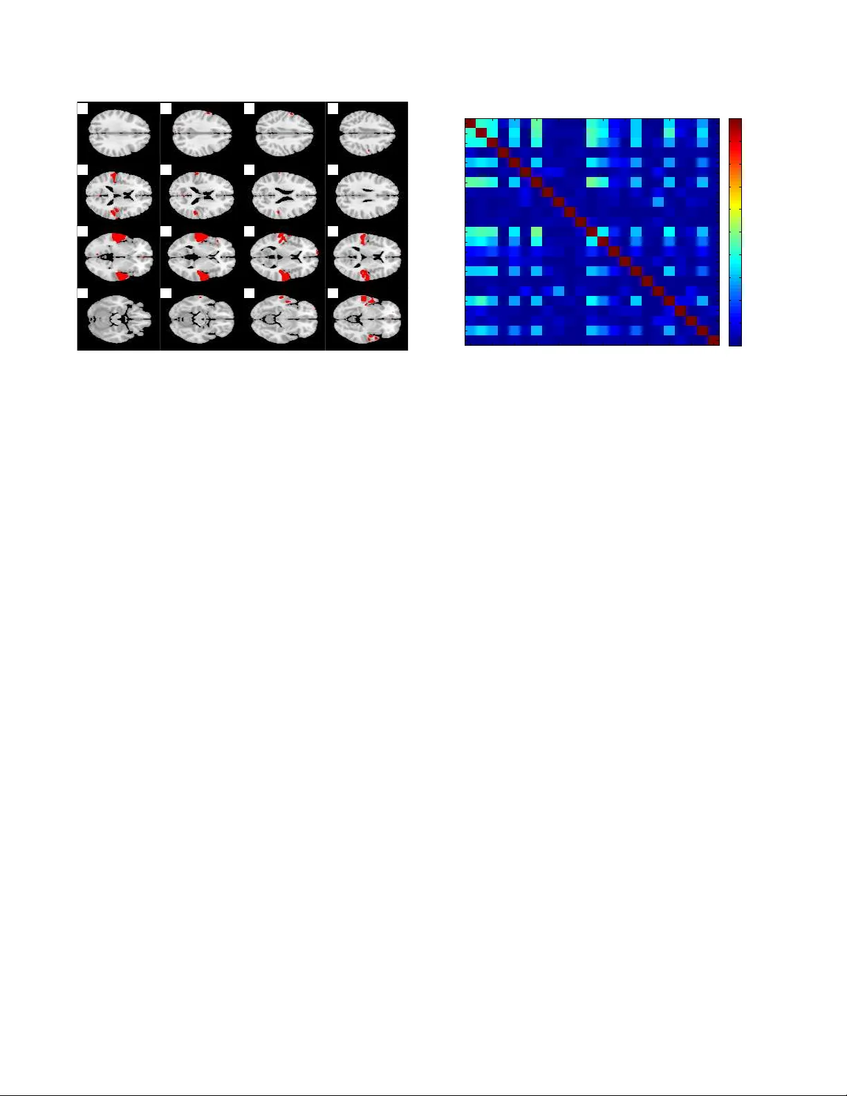
DIFFUSION MAP FOR CLUSTERING FMRI SP A TIAL MAPS EXTRA CTED BY INDEPENDENT COMPONENT ANAL YSIS T uomo Sipola 1 , ∗ , F engyu Cong 1 , † , T apani Ristaniemi 1 , V inoo Alluri 1 , 2 , P etri T oiviainen 2 , Elvira Br attico 2 , 4 , 5 , Asoke K. Nandi 3 , 1 , ‡ 1 Department of Mathematical Information T echnology , Uni versity of Jyv ¨ askyl ¨ a, Finland 2 Finnish Centre of Excellence in Interdisciplinary Music Research, Uni versity of Jyv ¨ askyl ¨ a, Finland 3 Department of Electronic and Computer Engineering, Brunel Uni versity , United Kingdom 4 Cogniti ve Brain Research Unit, Institute of Beha vioral Sciences, Uni versity of Helsinki, Finland 5 Brain & Mind Laboratory , Biomedical Engineering and Computational Science, Aalto Uni versity , Espoo, Finland ABSTRA CT Functional magnetic resonance imaging (fMRI) produces data about activity inside the brain, from which spatial maps can be extracted by independent component analysis (ICA). In datasets, there are n spatial maps that contain p vox els. The number of voxels is very high compared to the number of analyzed spatial maps. Clustering of the spatial maps is usually based on correlation matrices. This usually works well, although such a similarity matrix inherently can explain only a certain amount of the total variance contained in the high-dimensional data where n is relatively small but p is large. F or high-dimensional space, it is reasonable to perform dimensionality reduction before clustering. In this research, we used the recently dev eloped dif fusion map for dimen- sionality reduction in conjunction with spectral clustering. This research re v ealed that the dif fusion map based clustering worked as well as the more traditional methods, and produced more compact clusters when needed. Index T erms — clustering, dif fusion map, dimensionality reduction, functional magnetic resonance imaging (fMRI), in- dependent component analysis, spatial maps ∗ T uomo Sipola’ s work was supported by the Foundation of the Nokia Corporation and the Finnish Foundation for T echnology Promotion. † This work was partially supported by TEKES (Finland) grant 40334/10 Machine Learning for Future Music and Learning T echnologies. ‡ Asoke K. Nandi would like to thank TEKES for the award of the Finland Distinguished Professorship. 1. INTR ODUCTION In order to gain understanding about the human brain, var - ious technologies hav e recently been introduced, such as electroencephalography (EEG), tomography , magnetoen- cephalography (MEG) and functional magnetic resonance imaging (fMRI). They provide scientists with data about the temporal and spatial activity inside the brain. Functional magnetic resonance imaging is a brain imaging method that measures blood oxygenation lev el. It detects changes in this lev el, that are believed to be related to neurotransmitter activity . This enables the study of brain functioning, patho- logical trait detection and treatment response monitoring. The method localises brain function well, and thus is useful in detecting differences in subject brain responses [1, 2]. Deeper understanding about the simultaneous activities in the brain begins with a decomposition of the data. Indepen- dent component analysis (ICA) has been extensiv ely used to analyze fMRI data. It tries to decompose the data into multi- ple components that are mix ed in the original data. Basically , there are two ways to perform ICA: group ICA and individual ICA [3]. Group ICA is performed on the data matrix includ- ing all the participants’ fMRI data, and indi vidual ICA is ap- plied on each dataset of each participant. Among datasets of different participants, group ICA tends to need more assump- tions which are not required by indi vidual ICA [4]. For indi- vidual ICA, if the components for each participant are kno wn, it is expected to find the most common components among the participants. Therefore, clustering spatial maps extracted by ICA is a necessary step for the individual ICA approach to c  2013 IEEE. This is the authors’ postprint version of the article. The original print version appeared as: Tuomo Sipola, Fengyu Cong, T apani Ristaniemi, V inoo Alluri, Petri T oi viainen, Elvira Brattico, and Asoke K. Nandi. Diffusion map for clustering fMRI spatial maps extracted by independent component analysis. In Machine Learning for Signal Processing (MLSP), 2013 IEEE International W orkshop on, Southampton, United Kingdom, September 2013. IEEE. find common spatial information across dif ferent participants in fMRI research. ICA decomposes the indi vidual datasets and creates com- ponents that can be presented with spatial maps. After ICA has been applied, a data matrix of size n by p is produced, where n is the number of spatial maps and p is the number of vox els of each spatial map. The n spatial maps come from different participants, and n is much smaller than p in fMRI research. Clustering the spatial maps is mostly done using the n by n similarity matrix of the n by p data matrix [3, 5]. Surprisingly , it usually works well although such a similar- ity matrix inherently can just explain a certain amount of the total variance contained in the high-dimensional n by p data matrix [5]. New mathematical approaches for functional brain data analysis should take into account the characteristics of the data analyzed. As stated, spatial maps ha ve high dimensional- ity p . In machine learning, dimensionality reduction is usually performed on such datasets before clustering. In the small- n - large- p clustering problem, the con ventional dimensionality reduction methods, for example, principal component analy- sis (PCA) [6], might not be suitable for the non-linear prop- erties of the data. In this research, we apply a recently de- veloped non-linear method called diffusion map [7, 8] for di- mensionality reduction. The probabilistic background of the diffusion distance metric will gi ve an alternativ e angle to this dataset by facilitating the clustering task and providing vi- sualization. This paper explores the possibility of using the diffusion map approach for fMRI ICA component clustering. 2. METHODOLOGY This paper considers a dimensionality reduction approach to clustering of high-dimensional data. The clustering procedure flows as follo ws: 1. Data normalization with logarithm 2. Neighborhood estimation 3. Dimensionality reduction with dif fusion map 4. Spectral clustering Data normalization should be done if the features are on differing scales. This ensures that the distances between the data points are meaningful. Neighborhood estimation for dif- fusion map creates the neighborhood where connections be- tween data points are considered. Dimensionality reduction creates a new set of fe wer features that still retain most infor- mation. Spectral clustering groups similar points together . W e assume that our dataset consists of vectors of real numbers: X = { x 1 , x 2 , . . . , x n } , x i ∈ R p . In practice the dataset is a data matrix of size n × p , whose rows represent the samples and columns the features. In this study each row vector is a spatial map and column vector contains the corre- sponding vox els in different spatial maps. 2.1. Diffusion map Diffusion map is a dimensionality reduction method that em- beds the high-dimensional data to a low-dimensional space. It is part of the manifold learning method family and can be characterized with its use of diffusion distance as the pre- served metric [7]. The initial step of the diffusion map algorithm itself cal- culates the affinity matrix W , which has data vector distances as its elements. Here Gaussian k ernel with Euclidean distance metric is used [7, 9]. For  selection, see below . The affinity matrix is defined as W ij = exp  − || x i − x j || 2   , where x i is the p -dimensional data point. The neighborhood size parameter  is determined by finding the linear region in the sum of all weights in W , while trying different values of  [10, 11]. The sum is L = n X i =1 n X j =1 W i,j , From the affinity matrix W the row sum diagonal matrix D ii = P n j =1 W ij , i ∈ 1 . . . n is calculated. The W matrix is then normalized as P = D − 1 W . This matrix represents the transition probabilities between the data points, which are the samples for clustering and classification. The conjugate ma- trix ˜ P = D 1 2 P D − 1 2 is created in order to find the eigen v alues of P . In practice, substituting P , we get ˜ P = D − 1 2 W D − 1 2 . This so-called normalized graph Laplacian [12] preserves the eigenv alues [9]. Singular value decomposition (SVD) ˜ P = U Λ U ∗ yields the eigen values Λ = diag ([ λ 1 , λ 2 , . . . , λ n ]) and eigenv ectors in matrix U = [ u 1 , u 2 , . . . , u n ] . The eigen- values of P and ˜ P stay the same. It is now possible to find the eigen vectors of P with V = D − 1 2 U [9]. The low-dimensional coordinates in the embedded space Ψ are created using Λ and V : Ψ = V Λ . Now , for each p -dimensional point x i , there is a corre- sponding d -dimensional coordinate, where d  p . The num- ber of selected dimensions depends on how fast the eigen v al- ues decay . The coordinates for a single point can be expressed as Ψ d : x i → [ λ 2 v 2 ( x i ) , λ 3 v 3 ( x i ) , . . . , λ d +1 v d +1 ( x i )] . (1) The diffusion map now embeds the data points x i while preserving the diffusion distance to a certain bound gi ven that enough eigen v alues are taken into account [7]. 2.2. Spectral clustering Spectral clustering is a method to group samples into clusters by benefitting from the results of spectral methods that rev eal the manifold, such as the dif fusion map. Spectrum here is understood in the mathematical sense of spectrum of an op- erator on the matrix P . The main idea is that the dimension- ality reduction has already simplified the clustering problem so that the clustering itself in the lo w-dimensional space is an easy task. This leaves the actual clustering for any clustering method that can work with real numbers [13, 14, 15]. The first fe w dimensions from the dif fusion map represent the data up to a relativ e precision, and thus contain most of the distance differences in the data [7]. Therefore, some of the first dimensions will be used to represent the data. Threshold at 0 in the embedded space divides the space between the pos- sible clusters, which means that a linear classification can be used. W ith the linear threshold, the second eigen vector sepa- rates the data into two clusters in the low-dimensional space. This eigen vector solves the normalized cut problem, which means that there are small weights between clusters but the in- ternal connections between the members inside the cluster are strong. Clustering in this manner happens through similarity of transition probabilities between clusters [13, 14, 16, 17]. 3. RESUL TS The data comes from e xperiments where participants listened to music. The data analysis was performed on a collection of spatial maps of brain activity . After dimensionality reduc- tion and spectral clustering, the results are presented and com- pared to more traditional methods. 3.1. Data description In this research the fMRI data are based on the data sets used by Alluri et al. [18]. Elev en musicians listened to a 512- second modern tango music piece during the experiment. In the free-listening experiment the expectation was to find rel- ev ant brain activity significantly correlating with the music stimulus. The stimuli were represented by musical features used in music information retriev al (MIR) [18]. After preprocessing, PCA and ICA were performed on each dataset of each participant, and 46 ICA components (i.e., spatial maps) were extracted for each dataset [19, 20]. Then, temporal courses of the spatial maps were correlated with one musical feature, Brightness [18]. As long as the correlation coefficient was significant (statistical p -value < 0 . 05 ), the spatial maps were selected for further analysis. Altogether, n = 23 spatial maps were selected from 11 participants. The number of voxels for each spatial map was p = 209 , 633 . So, the 23 by 209,633 data matrix was used for the clustering to find the common spatial map across the 11 participants. 10 −10 10 −5 10 0 10 5 10 10 10 1 10 2 10 3 The weight matrix sum as a function of epsilon ε L Fig. 1 . Selecting  for diffusion map. The red line shows the selected value. 3.2. Data analysis The data matrix was analyzed using the methodology ex- plained in Section 2. The dimensionality of the dataset was reduced and then the spectral clustering was carried out. The weight matrix sum for  selection is in Figure 1; the used value is in the middle region, highlighted with straight verti- cal line. Clustering was performed with only one dimension in the low-dimensional space. T o compare the results with more traditional clustering methods, the high-dimensional data was clustered with agglomerativ e hierarchical clustering [21] with Euclidean distances using the similarity matrix [5] and k -means algorithms [21]. The clustering results for two clusters were identical using all the methods. Figure 2 shows the resulting clustering from the diffu- sion map. The figure uses the first two eigenpairs for low- dimensional presentation, for these two clusters ev en one di- mension is enough. The spatial maps are numbered and the two clusters are marked with different symbols. The divid- ing spectral clustering line is at 0 along the horizontal axis, so the point to the right of 0 are in one cluster and to the left another . T w o clusters, dense and sparse, are detected using this threshold. The dense cluster , marked with crosses, con- tains components that are considered to be similar according to this clustering. The traditional PCA and kernel PCA with Gaussian kernel for spectral clustering are compared to the diffusion map [22, 23]. In Figure 3 diffusion map with cor- rect  creates more firm connections, which eases the cluster- ing task. The effect of dif fusion distance metric is also seen. In Figure 4 the dendrogram produced by the agglomera- tiv e clustering is shown. The clustering results are the same as with the dimensionality reduction approach. The separation is visible at the highest lev el and the structure corresponds −1 −0.5 0 0.5 −0.8 −0.6 −0.4 −0.2 0 0.2 0.4 0.6 2nd eigenpair 3rd eigenpair Clustering in low dimensions, components numbered 1 2 3 4 5 6 7 8 9 10 11 12 13 14 15 16 17 18 19 20 21 22 23 Sparse cluster Dense cluster Fig. 2 . Diffusion map clustering results. −1 −0.5 0 0.5 −1 −0.5 0 0.5 PCA −1 −0.5 0 0.5 −1 −0.5 0 0.5 kPCA −1 −0.5 0 0.5 −1 −0.5 0 0.5 Diffusion map Fig. 3 . Dimensionality reduction method comparison. The coordinates hav e been scaled. to the distances seen in Figure 2. All the points in, e.g., the dense cluster in Figure 2 are in the left cluster of Figure 4. This comparison shows the evident separation between the two clusters and also v alidates the results from diffusion map methodology . Figure 5 illustrates the kind of spatial maps that are found in the dense cluster . Dark areas along the lateral sides is used to highlight those voxels whose values dif fered more than three standard deviations from the mean. The numbers marking the slices are their Z-coordinates. The correspond- ing low-dimensional point is in Figure 2 numbered as 3. It is now possible to inspect the clusters more closely with domain experts. Figure 6 shows the correlation matrix of all the 23 spatial maps. This is a way to inspect the similarity of the brain ac- tivity . The correlation matrix is also the basis of analysis for the hierarchical clustering [5]. In the figure it can be seen that there is some correlation between some of the spatial maps, but not so much between others. Figures 7 and 8 illustrate the internal structure of the clus- ters by showing the correlation matrices for the individual clusters. The members in the dense cluster have higher cor- 7 12 2 1 3 13 5 16 19 22 4 14 8 20 23 10 15 17 21 6 9 18 11 1.05 1.1 1.15 1.2 1.25 1.3 1.35 1.4 1.45 1.5 Dendrogram from agglomerative clustering Data points Distance between data points Fig. 4 . Dendrogram from the agglomerativ e clustering. relation among themselves than the members in the sparse cluster . This information is also seen in Figure 2 where the diffusion distances inside the dense cluster are smaller . 4. DISCUSSION In this paper we ha ve proposed a theoretically sound non- linear analysis method for clustering ICA components of fMRI imaging. The clustering is based on diffusion map manifold learning, which reduces the dimensionality of the data and enables clustering algorithms to perform their task. This approach is more suitable for high-dimensional data than just applying clustering methods that are designed for low- dimensional data. The assumption of non-linear nature of brain activity also promotes the use of methods designed for such problems. P articularly , the advantage of diffusion map is in visualizing the distribution of all data samples ( n spatial maps with p voxels in each) by using only two coordinates. As seen in the visualization, it becomes more straightforward to determine the compact cluster from the two-dimensional plot deri ved from the 209,633-dimensional feature space than from the similarity matrix. The results show that the proposed methodology separates groups of similarly behaving spatial maps. Results from dif- fusion map spectral clustering are similar to hierarchical ag- glomerativ e clustering and k -means clustering. Small sam- ple size and good separation of clusters makes the clustering problem rather simple to solve. Moreov er , the visualization obtained from diffusion map of fers an interpretation for clus- tering. The proposed methodology should be useful for analyzing the function of the brain and understanding which stimuli cre- ate similar spatial responses in which group of participants. 28 30 32 34 36 38 40 42 44 46 48 50 52 54 56 58 Component #3 Dense cluster Fig. 5 . Example spatial map in the dense cluster , this is data point number 3. Dark lateral areas mark more than three stan- dard deviations from the mean, e.g. in slices 36 and 38. The domain experts can gain more basis for the interpretation of brain activity when similar activities are already clustered using automated processes suitable for the task. Furthermore, visualization helps to identify the relationships of the clusters. Diffusion map e xecution times become increasingly larger if the number of samples goes very high. This can be overcome to a certain degree with out-of-sample exten- sion. Big sample sizes are also a problem with traditional clustering methods. Howe ver , diffusion map of fers a non- linear approach, and is suitable for high-dimensional d ata. Both properties are true for fMRI imaging data. The analysis could be expanded to more musical features and to bigger datasets in order to further validate its useful- ness in understanding the human brain during listening to music. The method is not restricted only to certain kind of stimulus, so it is usable with div erse fMRI experimental se- tups. Furthermore, situations where traditional clustering fails when processing spatial maps, the proposed methdodology might giv e more reasonable results. 5. REFERENCES [1] P M Matthe ws and P Jezzard, “Functional magnetic res- onance imaging, ” Journal of Neur ology , Neur osur gery & Psychiatry , v ol. 75, no. 1, pp. 6–12, 2004. [2] S. A. Huettel, A. W . Song, and G. McCarthy , Functional Magnetic Resonance Imaging , Sinauer, Massachusetts, 2nd ed. edition, 2009. [3] V ince D Calhoun, Jingyu Liu, and T ¨ ulay Adalı, “ A re- view of group ICA for fMRI data and ICA for joint in- ference of imaging, genetic, and ERP data, ” Neur oim- age , v ol. 45, no. 1 Suppl, pp. S163, 2009. Spatial map Spatial map Correlation matrix 1 3 5 7 9 11 13 15 17 19 21 23 1 2 3 4 5 6 7 8 9 10 11 12 13 14 15 16 17 18 19 20 21 22 23 Absolute correlation value 0 0.1 0.2 0.3 0.4 0.5 0.6 0.7 0.8 0.9 1 Fig. 6 . Absolute correlation values between the spatial maps. [4] Fengyu Cong, Zhaoshui He, Jarmo H ¨ am ¨ al ¨ ainen, Paa vo H.T . Leppnen, Heikki L yytinen, Andrzej Ci- chocki, and T apani Ristaniemi, “V alidating rationale of group-level component analysis based on estimating number of sources in EEG through model order selec- tion, ” Journal of Neur oscience Methods , vol. 212, no. 1, pp. 165–172, 2013. [5] Fabrizio Esposito, T ommaso Scarabino, Aapo Hyvari- nen, Johan Himberg, Elia Formisano, Silvia Comani, Gioacchino T edeschi, Rainer Goebel, Erich Seifritz, Francesco Di Salle, et al., “Independent component analysis of fMRI group studies by self-organizing clus- tering, ” Neuroima ge , v ol. 25, no. 1, pp. 193–205, 2005. [6] Ian Jolliffe, Principal component analysis , Springer V erlag, 2002. [7] Ronald R. Coifman and St ´ ephane Lafon, “Diffusion maps, ” Applied and Computational Harmonic Analysis , vol. 21, no. 1, pp. 5–30, 2006. [8] B. Nadler , S. Lafon, R.R. Coifman, and I.G. K evrekidis, “Diffusion maps, spectral clustering and reaction coor- dinates of dynamical systems, ” Applied and Computa- tional Harmonic Analysis , vol. 21, no. 1, pp. 113–127, 2006. [9] Boaz Nadler , Stephane Lafon, Ronald Coifman, and Ioannis G. Ke vrekidis, “Diffusion maps – a proba- bilistic interpretation for spectral embedding and clus- tering algorithms, ” in Principal Manifolds for Data V i- sualization and Dimension Reduction , T imothy J. Barth, Michael Griebel, Da vid E. K eyes, Risto M. Niemi- nen, Dirk Roose, T amar Schlick, Ale xander N. Gor- ban, Bal ´ azs K ´ egl, Donald C. W unsch, and Andrei Y . Spatial map Spatial map Correlation matrix for dense cluster 1 2 3 5 7 12 13 16 19 22 1 2 3 5 7 12 13 16 19 22 Absolute correlation value 0 0.1 0.2 0.3 0.4 0.5 0.6 0.7 0.8 0.9 1 Fig. 7 . Absolute correlation values between the spatial maps that belong to the dense cluster . Zinovye v , Eds., vol. 58 of Lecture Notes in Computa- tional Science and Engineering , pp. 238–260. Springer Berlin Heidelberg, 2008. [10] R.R. Coifman, Y . Shkolnisky , F .J. Sigworth, and A. Singer , “Graph laplacian tomography from unknown random projections, ” Image Pr ocessing, IEEE T ransac- tions on , vol. 17, no. 10, pp. 1891–1899, oct. 2008. [11] Amit Singer, Radek Erban, Ioannis G. Ke vrekidis, and Ronald R. Coifman, “Detecting intrinsic slow variables in stochastic dynamical systems by anisotropic dif fusion maps, ” Pr oceedings of the National Academy of Sci- ences , vol. 106, no. 38, pp. 16090–16095, 2009. [12] F . R. K. Chung, Spectral Graph Theory , p. 2, AMS Press, Providence, R.I, 1997. [13] Andre w Y . Ng, Michael I. Jordan, and Y air W eiss, “On spectral clustering: Analysis and an algorithm, ” in Ad- vances in Neural Information Pr ocessing Systems 14 . 2001, pp. 849–856, MIT Press. [14] Ravi Kannan, Santosh V empala, and Adrian V etta, “On clusterings: Good, bad and spectral, ” J. ACM , vol. 51, pp. 497–515, May 2004. [15] Ulrike von Luxb urg, “ A tutorial on spectral clustering, ” Statistics and Computing , vol. 17, pp. 395–416, 2007. [16] Jianbo Shi and J. Malik, “Normalized cuts and image segmentation, ” P attern Analysis and Machine Intelli- gence, IEEE T ransactions on , v ol. 22, no. 8, pp. 888 –905, 2000. [17] Marina Meila and Jianbo Shi, “Learning segmentation by random walks, ” in NIPS , 2000, pp. 873–879. Spatial map Spatial map Correlation matrix for sparse cluster 4 6 8 9 10 11 14 15 17 18 20 21 23 4 6 8 9 10 11 14 15 17 18 20 21 23 Absolute correlation value 0 0.1 0.2 0.3 0.4 0.5 0.6 0.7 0.8 0.9 1 Fig. 8 . Absolute correlation values between the spatial maps that belong to the sparse cluster . [18] V inoo Alluri, Petri T oiviainen, Iiro P J ¨ a ¨ askel ¨ ainen, En- rico Glerean, Mikko Sams, and Elvira Brattico, “Large- scale brain networks emerge from dynamic processing of musical timbre, key and rhythm, ” Neur oimage , vol. 59, no. 4, pp. 3677–3689, 2012. [19] T . Puoliv ¨ ali, F . Cong, V . Alluri, Q. Lin, P . T oiviainen, A. K. Nandi, E. Brattico, and T . Ristaniemi, “Semi- blind independent component analysis of functional MRI elicited by continuous listening to music, ” in Inter - national Confer ence on Acoustics, Speech, and Signal Pr ocessing 2013 (ICASSP2013) , V ancouver , Canada, May 2013. [20] V aleri Tsatsishvili, Fengyu Cong, T uomas Puoli v ¨ ali, V i- noo Alluri, Petri T oiviainen, Asoke K Nandi, Elvira Brattico, and T apani Ristaniemi, “Dimension reduc- tion for individual ICA to decompose fMRI during real- world experiences: Principal component analysis vs. canonical correlation analysis, ” in Eur opean Symposium on Artificial Neural Networks 2013 , Bruges, Belgium, April 2013. [21] Rui Xu, Donald Wunsch, et al., “Survey of clustering algorithms, ” Neural Networks, IEEE T ransactions on , vol. 16, no. 3, pp. 645–678, 2005. [22] K-R M ¨ uller , Sebastian Mika, Gunnar R ¨ atsch, K oji Tsuda, and Bernhard Sch ¨ olkopf, “ An introduction to kernel-based learning algorithms, ” Neur al Networks, IEEE T ransactions on , v ol. 12, no. 2, pp. 181–201, 2001. [23] Quan W ang, “K ernel principal component analysis and its applications in face recognition and acti ve shape models, ” arXiv preprint , 2012.