On the Asymptotic Validity of the Decoupling Assumption for Analyzing 802.11 MAC Protocol

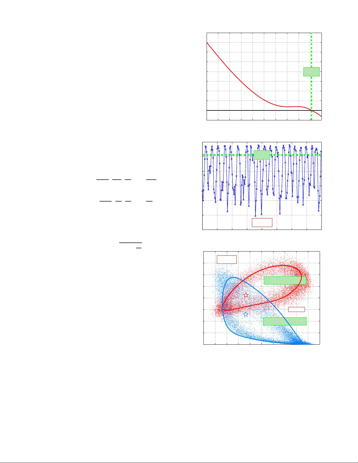
1 On the Asymp totic V alidity of the Decoupling Assumption for Analyzing 802. 11 MA C Protocol Jeong-woo Cho, Jean -Yves Le Bou dec, F ellow , IEEE, and Y uming Jian g Abstract —Perf ormance ev aluation of the 802.11 MA C pro- tocol is classically based on th e decouplin g assumption, which hypothesizes that th e backoff processes at di fferent nodes are independ ent. This d ecoupling assumption results from mean field con ver gence and is generally true in transient regime in the asymptotic sense (when the number of wireless nodes tends to infinity), but, contrary to widespread belief, may not n ecessarily hold in stationary regime. Th e issue is often related with the existence and un iqueness of a solution to a fixed poin t equation ; howev er , it was also recently sh own that this conditi on is not sufficient; in contrast, a sufficient condition is a global stability property of the associated ordin ary differential equation. In this paper , we giv e a simple condition that establish es the asymptotic validity of th e decouplin g assumption for the homogeneous case. W e also d iscuss th e h eteroge neous and the differentiated service cases and f ormulate a new ordin ary d ifferential equation. W e show that th e u niqueness of a solu tion to the associated fixed point equ ation is not sufficient; we exhib it one case where the fixed point equation has a uniqu e solution but the d ecoupling assumption is not valid i n the asymptotic sense in stationary regime. Index T erms —Mean field theory , ordinary dif ferential equ a- tion, fi xed p oint equation, 802.11, decoupling assumption . I . I N T R O D U C T I O N T HE W ireless LAN standa rd is evolving tow ards h igher and high er aggregate throughp ut. The increased max- imum bit r ate of 8 02.11n , 600 Mbps, along with its easy deployability , sugg ests the potential use o f an 80 2.11n access point as an wir eless ro uter tra nsacting a hu ge am ount of data of many nod es. In this work, we focu s on the per forman ce ev aluation of 80 2.11 u nder the many-nod e re gime as the populatio n size (th e n umber of wireless node s) N tends to infinity . Most existing work on performanc e e valuation of the 802.11 MA C proto col [2], [11], [1 2], [18] relies on the “deco upling assumption” wh ich was first ado pted in the seminal work by Bianchi [2]. Th ough h aving b een defined in various ways, it essentially assumes that all the nodes in the same network experience the same time-invariant collision prob ability , with This work was supporte d in part by “Centr e for Quantifiabl e Quali ty of Service in Communicatio n Systems, Centre of Excellence ” appointed by The Researc h Counci l of Norway , and funded by The Researc h Council, NT NU and UNINETT . A part of this work was done when J. Cho was with E PFL, Switzerl and. J. Cho is with the School of Information and Communication T echnol- ogy at KT H Royal Institute of T echnology , Stockholm, Sweden (email: jwcho@kt h.se). J.-Y . Le Boudec is with ´ Ecole Polytechniq ue F ´ ed ´ e rale de Lausanne (EPFL), CH-1015 L ausanne, Switzerl and (email: jean-yves.le boudec@epfl.ch) . Y . J iang is with the Department of T elematics, Norwegi an Univ ersity of Science and T echnology (NTN U), N-7491, Trondhe im, Norway . (email: jiang@i tem.ntnu.no). the direct conseque nce that the bac koff processes ar e indepen- dent 1 . This assumption is u nav oidable primarily because the stationary distribution o f the orig inal Mar kov chain canno t be explicitly written d ue to the irr ev ersibility of the chain [12] ev en for small numb er of backoff stages, i.e. , 3 and 4 , un less the po pulation of the network is very small. A similar point was stressed by P . R. K umar in an inter view with Science W atch Newsl etter [1 3]: ”A go od analogy is in thermodyn amics. Instead of trying to study the behavior of just thr ee or four molecules and how the y move ar o und, you study the behavior of billions and trillions of molecules. . . . Similarly , we want to see what you can say about wir eless networks in the aggr e gate. ” which suggests an analogy of the intractable small-scale problem s in different areas. If we liken each wir eless no de to a particle in a p hysical system, wh ich co ndition would suffice for ev ery particle being absolutely decou pled from the rest? Once we a ssume that the decoup ling assump tion holds, the analysis of th e 8 02.11 MAC proto col leads to a fixed p oint equation (FPE) [12], also called Bianchi’ s formula. Kumar et al. [ 12] revisited the FPE an d m ade several r emarkab le o bser- vations, adv ancing th e state of the a rt to m ore systematic mod- els and paving the way for m ore com prehensive understand ing of 802 .11. Above all, one o f the key findin gs of [ 12], alre ady adopted in th e field [ 15], [1 8], is that th e full interference model, also called th e single-cell model [1 2] and the main focus of our work, leads to the back off synchr ony pr op erty [17] which implies the backoff process can be comp letely separated and analyzed solely throug h the FPE techniq ue. This deco upling assumption c an be fo rmally justified as a consequen ce of convergence to me an field and of Sznitman ’ s result [23]; it can thus only be asym ptotically true as the populatio n N goes to in finity . Howev er, it is recently p ointed out by Bena ¨ ım and Le Boud ec [1, Sec tion 8.2] tha t Sznitman ’ s result and c on vergence to m ean field imp ly the asym ptotic validity o f the dec oupling assumption on ly in the transient regime, i.e . , over a finite ho rizon, and gi ven some initial condition s. In stationary regime, there m ay be no decoup ling assumption e ven in the limit of large popu lation size N . This may happ en f or example when the ord inary differential equation ( ODE) that defines the mean field limit has a limit cycle. In such a case, n odes are asy mptotically ind ependen t only conditiona l to the state of the fluid limit. In contrast, if the ODE satisfies a stron g global stability prop erty , namely , it has 1 The meaning of “to decouple ” in the literat ure as well as in our work is an abuse of terminology , in the sense that it has implied not only ‘to decoupl e nodes’ (independ ence) but also ‘to have a time-in v ariant collision probability ’. 2 a u nique stationary point to which all trajec tories converge, then the decou pling assumption is also valid in stationar y regime [1]. For the c ase of the 802.11 MA C proto col, the stationary po ints of the ODE are the solutio ns of the FPE mentioned above. Howe ver, existence and uniq ueness of a solution to the FPE does n ot guaran tee that all trajec tories of the ODE conv erge to the unique fixed p oint; in [1], th ere is a simple example of mean field limit wher e th e FPE h as a unique so lution but trajecto ries of th e ODE do not co n verge, in gen eral, to this uniqu e fixed p oint. Theref ore, th ough the decoup ling assumption s that underly Bianc hi’ s fo rmula is plausible and intuiti ve, the question of its v alidity can be asked. The main purpo se o f this p aper is to provide an answer to the following qu estion. “Under which conditio ns is the decoupling assumption for the model of the 802.11 MA C asymptotically valid?” T o put it another way , we ask wh ether the FPE metho d and Bianchi’ s assumption are valid. T o this end, we use mean field theoretic results [ 1], [7], [22] which state that, as N ten ds to infinity , a scaled version o f the original Markov chain m odel of the backoff p rocess in 8 02.11 MA C pro tocol conv erges to a nonlinear or dinary differ ential equa tion (ODE ) so th at the asymptotic validity of the decou pling assumptio n an d thus o f the FPE boils down to the stability of this ODE. Den oting by p k the attem pt prob ability of each wireless node at each time- slot in backoff stage k ∈ { 0 , 1 , · · · , K } , we assume in w hat follows th at ou r mean field models ar e d eriv ed when K is finite and fixed wh ile the n umber of nod es N g oes to infinity . In connection with the mean field mo dels, it is worth while to clarify why th e relev ant works [1], [7], [2 2] have used a specific intensity scalin g regime, under which th e activity o f each node in backoff stage k is scaled as fo llows: p k := ǫ ( N ) · q k ( q k is a constan t.) (1) where q k is called the scaled attempt rate through out this paper . It is na tural to assume that ǫ ( N ) is vanishing , i.e. , lim N →∞ ǫ ( N ) = 0 . Otherwise, the co llision probab ility between wireless nodes c on verges to on e as N goes to infinity . Mo re impor tantly , we have to use a n app ropriate form of intensity scaling ǫ ( N ) in order to av oid exceptional cases. For example, if ǫ ( N ) decr eases faster than 1 / N ( e.g. , ǫ ( N ) = 1 / N 2 ), it can be easily seen th at th e co llision probab ility vanishes as N tends to infinity , irrespective of whichever backoff stage e ach node be longs to (we r efer to Section II- E for a formal argument). In other words, eac h node is completely deco upled fr om th e rest. On the other h and, if ǫ ( N ) decreases slo wer than 1 / N ( e.g. , ǫ ( N ) = 1 / √ N ), the collision probab ility beco mes on e as N goe s to infinity . That is to say , ǫ ( N ) = 1 / N is the o nly intensity scaling r egime (u p to a constant factor) that deserves to b e analyzed. Under th e intensity scaling regime ǫ ( N ) = 1 / N , Bord enave et al. in [7, Theorem 5. 4] studied th e homogeneous case (all n odes hav e th e same per-stage backoff pro babilities) for the case whe n the numb er of backoff stages is infinite. They found the f ollowing sufficient con dition for global stability of the ODE, hen ce for the a symptotic validity of the d ecouplin g assumption: q 0 < ln 2 and q k +1 = q k / 2 , ∀ k ≥ 0 (BMP) where q k is the scaled attempt rate in (1) f or a no de in backoff stage k . In th is paper, we focus on the case w here the total nu mber of backoff stages K + 1 is finite, as this is true in practice and in Bianch i’ s formu la. Shar ma et al. [22] obtained a result for K = 1 and mentioned the diffi culty to go beyond. A compr ehensive summary of the literature and the outstanding qu estions raised therein h as been rec ently made by Duffy [9]. W e find that not on ly (i) the mon otonicity ((MONO) in Section II) but also (ii) the mild intensity o f scaled attempt rates ((MINT) in Section II) imply the uniqueness of a solution to the FPE, which is natu rally a nece ssary cond ition f or stability . Moreover , we prove that the latt er (MINT) guara ntees the global stability of the ODE. T hus the condition that the attemp t rate is upper-bound ed by the recipr ocal of th e populatio n, namely q k ≤ 1 fo r all k , suffices f or th e validity of the de coupling a ssumption. Moreover , f or the familiar parameter setting q k = q 0 /m k where m ≥ 1 , the cond ition (MINT) suffices f or ma ximizing the aggr egate through put of the network, h ence it is a practical condition . In order to o ffer various servic es to hig her pr iority u sers with a dditional per formanc e requ irements, 802 .11e standard introdu ced the en hanced distributed chan nel access (EDCA) function ality th at has three mecha nisms to d ifferentiate the per-class settin gs o f ( i) chan nel holding tim e, ( ii) con tention window (CW), and ( iii) idle time af ter each transmission, where th e first on e has no effect o n the backoff pr ocesses. Since the second one, CW differentiation, n ecessarily implies there are two or mo re classes, we call th e corr espondin g system heterogeneo us . The th ird o ne, called AIFS differenti- ation, imposes an additio nal complexity on the Markov ch ain analysis beca use whether the users of a class may attempt transmission at each time-slot depe nds on the type of the current time-slot, which again dep ends on the activity of the users in the previous time -slot. Th is mu tual interaction of the two ev olutio ns sub stantially com plicates the analysis. As o f now , there is no ODE in the literature which m odels AIFS differentiation using an appr opriate fo rmalism. T o tackle this problem, it is of importance to observe that the stage ev olution of all nodes (or stag e density) is much slower than the ev olution of the ty pe of time-slots u nder the AIFS differentiation. Thu s the former can be taken to b e constant by the latter . An application of mean field theoretic result [1, Theorem s 1 & 2], formalized based on the same observation, yields an e xtended ODE model o f the b ackoff p rocesses in EDCA-enabled 80 2.11 networks. W e also formulate an extended FPE o n the ba sis of this ODE, which is satisfied by the equ ilibrium points of the ODE. I t is rema rkable th at this FPE coincides with that prop osed in [1 2, Section VI] . The versatility of the ODE model is demo nstrated by in ves- tigating some selected co unterexamples. In the first exam ple, we consid er a h omogen eous system where all n odes use the same parameter s an d show that the system is bistable in that the b ackoff process, after whirling closely arou nd a n equilibriu m for a very long time, sudd enly jumps into ano ther 3 equilibriu m, and vice versa . The FPE m odel is only cap able of identifyin g thre e equilib rium points as its solutions, whe reas the ODE model is furth er capable of classifying the two of them into loca lly stab le po ints an d the other into u nstable point, accurately reflecting the multistability . The trajectories of the ODE constitute a separ atrix wh ich divides the initial condition space into two regions. W e also co nsider a het- erogen ous system where the set o f no des ar e divided into two classes. A delicate determination of the parameters ren ders the system oscillatory such that all trajectories con verge to a stable limit cycle form ed ar ound an unstab le u nique equilibr ium point wher e the limit cycle is as determin ed by th e extended ODE. This example also serves as an illustration of the fact that there may be a uniq ue solu tion to the fixed point e quation whereas th e d ecoupling assump tion do es not ho ld in the asymptotic sense. W e also stress that the stability con dition established in this work for the first time has been tantalizing other researcher s as well, e.g. , [2 2, Appendix B]. The rest of th e p aper is organized as fo llows. In Section II, we pr esent a b rief overview of r ecent ad vances in me an field theory and introdu ce the associa ted ordin ary d ifferential equation th ereof. In Section III , we prove a g lobal stability condition of the ODE, which is in tu rn shown to b e capable of optim izing the throughp ut. In Section IV, we elaborate on anoth er c omplexities arising from EDCA an d derive its correspo nding ODE mo del. Some cou nterexamples in Section V illustrate the utility of the ODE models. Concluding remarks and an outstanding prob lem are given in Section VI. I I . M E A N F I E L D T E C H N I Q U E R E V I S I T E D T o begin with, it shou ld be noted that our analytical model of 802. 11 MA C pro tocol is different f rom th e o riginal one. Thus we first briefly describ e the orig inal o peration of 8 02.11 MA C in Section I I-A and explore the d ifferences between our model and the real 802 .11 MAC pro tocol in Section II -B. If the d uration of per-stage backoff is taken to be g eometric (which is u niform in the standard), the backoff pr ocess in 802.1 1 is governed by a few rules: ( i) every node in b ackoff stage k attempts transmission with probab ility p k for every time-slot; (ii) if it succeeds, k changes to 0 ; (iii) otherwise, k ch anges to ( k + 1) mo d ( K + 1) where K is the index of the highest backoff stage. Markov chain models, which have been wid ely used in describing com plex systems includin g 802.1 1, however , very often lead to excessiv e complications as discussed in Section I. In this section, we present a surrogate tool for the analysis, mean field th eory . I t is n otew orthy that the rules used in 802.1 1, i.e. , ( i)–(iii), closely resemble the mean field equatio ns laid out be low . A. Basic O peration of DCF Mode T ime is slotted . Since our analysis is mainly f ocused on th e backoff proc edure o f 802.1 1 distributed coor dination fun ction (DCF), we call the standardized time in terval in the backoff proced ure of the 80 2.11 standard time-slot 2 for brevity . The 2 This is equi val ent to s lot in the work by Kuma r et al. [12] ( e.g. , 20 µs in IEEE 802.11b). duration s of frames, packets, and in ter-frame spaces used in the oth er pro cedures are generally different from th at of a time-slot. Each n ode follows the rando mized ac cess pr ocedure of 802.1 1 DCF . T o begin with, each no de gen erates a backoff value if it has a d ata p acket to sen d. Since the backoff proced ure of each node is controlled by inter -frame spaces that fill in spaces between fram es and packets, we introduce the m here to help to under stand the basic o peration of DCF mode. T w o typ es of inter-frame spaces are used in 8 02.11 DCF , namely , Short Inter-Frame Space (SIFS) and Distrib uted Inter- Frame Space (DIFS). Each n ode freezes (stops) the countd own proced ure as soon a s the medium b ecomes busy . On the o ther hand, on ly when the medium is idle for th e dur ation of a Distributed Inter-Frame Space (DIFS), a node may u nfreeze (start) its co untdown pro cedure of the b ackoff and de crements the ba ckoff by o ne p er every time-slot. If the backoff reaches zero, the sender transmits an R T S (read y to send) fr ame, followed by a CTS (clear to send) fr om the r eceiv er, a da ta packet from the sender and an ACK packet from the recei ver if R TS/CTS mechanism is switched on. Note that SIFS is smaller than DIFS so that no node is allowed to interr upt a seq uence of frames and packets which are sp aced out SIFS apart. There e xist K +1 b ackoff stage s whose i ndices belon g to the set { 0 , 1 , · · · , K } wh ere K > 0 . If a nod e has not attempted transmission for a da ta packet yet, the node is supp osed to be in the initial bac koff stage wh ere the backoff value is dr awn unifor mly f rom { 0 , 1, · · · , 2 b 0 − 1 } ( or { 1, 2, · · · , 2 b 0 } ). Here 2 b 0 is the co ntention window that serves as the initial value of a backoff co untdown. I f two o r mo re wireless nodes finish their countdowns at the s ame time-slot, there occ urs a collision between R TS f rames if th e R TS/CTS mechanism is switched on, otherwise two or mor e d ata packets collide with each other . If there is a collision, each node who participated in the collision multiplies its contention window b y the multiplicative factor m = 2 . I n oth er words, ea ch node changes its backoff stage ind ex k to k + 1 a nd ad opts a new con tention wind ow 2 b k +1 = 2 m k +1 b 0 . If k + 1 is g reater than the in dex of the highest backoff stage number, K , the node steps bac k into the initial backoff stag e and the contention window is set to 2 b 0 . Let L and L c denote the average d uration of a suc cessful packet tran smission a nd the fixed d uration of a c ollision, expressed in terms of backoff time-slot. Note here th at th e length of data packets c an be arbitrary random values. Also the fixed overhead for each successful tran smission is deno ted by L o . Note that L , L c and L o do not need to be integer number s but can be arbitrar y positiv e r eal numb ers. In 80 2.11 DCF , if the R TS/CTS mechanism is used, L represents the time to transmit an R TS fra me, a CTS frame , a d ata packet, a nd an A CK pa cket plus inter-frame spaces, i.e. , SIFS and DIFS, where L o is L min us the time to tran smit a data p acket. Th e duration L c , much smaller than L , is the time to transmit an R TS frame plus one DIFS. B. Dif fer ences between Our Model and 802 .11 DCF Mode Our a nalysis is made tractable by a numb er of differences between our m odel u sed in th is pap er an d the orig inal op era- tion of 80 2.11 DCF mode. First of all, we take the d uration of 4 per-stage backoff to b e geometric as we did at the beginn ing of Section II. Seco ndly , the parameter set is fixed for each version of the standar d whe reas e ach pa rameter in o ur model may be an arbitrary number . For e xample , in the IEEE 802.11b standard, m = 2 , K = 6 ( 7 attemp ts per packet), and 2 b 0 = 32 are used. W e also make a fe w assumptio ns for tractab le an alysis. • Single- cell assumption : Most importantly , this work fo- cuses on the perform ance of sing le-cell 802. 11 networks in which all 802.11 -complian t n odes ar e within su ch a distance from e ach other that a node can hear whatever the other n odes transmit. Since all no des freeze their backoff co untdown durin g channel activity , the to tal time spent in backoff co untdowns up to any time is the same for all nodes. Therefo re, it is sufficient to an alyze the backoff pro cess in ord er to inv estigate the per forman ce of single-ce ll networks. This techn ique has been adop ted in many work s in cluding [1], [7], [12], [18]. • G reedy-node a ssumption : Secondly , we o nly consider the case of greedy wire less n odes tha t per sistently con - tend for the wireless mediu m. • Error-free channel assumption : Lastly , w e assume that the wireless c hannels ar e er ror-free so that failed trans- missions are cau sed only by collisions betwee n R TS frames (for the case of R TS/CTS) or d ata p ackets. C. Bianchi’ s F ormula In perform ance analysis of 802. 11, Bianchi’ s for mula an d its many v ariants are pro bably the most known [2], [8], [1 1], [12], [ 15], [1 6], [18], [ 20]. Assumin g that there ar e N nodes, Bianchi’ s formu la can be wr itten comp actly in a m ore gen eral fixed point equa tion (FPE) fo rm: ¯ p = P K k =0 γ k P K k =0 γ k p k , (2) γ = 1 − (1 − ¯ p ) N − 1 (3) where ¯ p and γ respectively designate the average attempt probab ility and collision pro bability o f every node at eac h time-slot. The attempt probability in backof f stage k is denoted by p k and defined as the inverse of th e m ean conten tion window , i.e. , p k = 1 / ( b k − 1 / 2 ) . Note that, as lo ng as th e backoff stage k = 0 follows b ackoff stage k = K for any attempts, the statistics like ¯ p and γ are no t affected by whether attempts in th e highest backoff stage K are successfu l o r not. The FPE mode l has been used a s a de facto prin cipal tool for the analysis of th e 802.1 1 MA C Protoco l. The weak po int of the FPE model is that it can not be co ncluded entirely from the for m of FPE wheth er its solution (even if it is unique) might be a good first-order appro ximation o f ¯ p and γ . Exactly und er which co ndition the FPE ho lds is r ecently being inv estigated with rigorou s m athematical arguments [1], [7], [22], called mean field in depend ence . Th is fu ndamenta l approa ch was originally developed in the two works by Bor- denave et al. [5] and Sharma et al. [21] wher e the first mean field ana lyses of the 802.1 1 MAC protocol were per formed 3 . 3 The conference versions of the two works were submitted at roughly the same times. In the rest of the paper, we will refer to th eir journal versions [7], [22]. Rema rkably , Bordenave et al. [ 7] provided a broa der mean field framework which extends to m ultiple-cell networks ( cf . single-cell assumption in Sec tion II-B) and suppor ts the notion of ‘ resource’. The par ticle in teraction model p roposed in [1] overcom es some limitation s and broad ens a pplicability of the m odel prop osed in [7]. Th e three works [1], [7], [2 2] have fou nd that, as th e num ber of particles go es to in finity , i.e. , N → ∞ , the stage distribution of every node e volves accordin g to a set of K + 1 d imensional nonlinear ordinary differ en tial equa tions (ODE) under an app ropriate scaling of time. D. Th e Mean F ield ODE mo del Let u s dive into the d etails of the mean field interactio n model for 802.1 1 used in [1], [7], [2 2] and h ow the Markov chain o f the mo del converges to th e associated or dinary differential equ ation. Model descript ion : In our version of 802.11 DC F mode under the assumption made in Section II-B, there are N wireless nodes ev olving in a finite state spa ce { 0 , · · · , K } at discre te time-slots t ∈ { 0 , 1 , · · · } . Den oting by X n ( t ) ∈ { 0 , · · · , K } the ba ckoff stage (the state) of nod e n ∈ { 1 , · · · , N } at time-slot t , we collect the o bservations X n ( t ) , for all n ∈ { 1 , · · · , N } and com pute the relativ e frequ encies, whic h is called the occupancy measure ( or empirical measure). For- mally , the occupa ncy measur e in backoff stage k at (discrete) time-slot t is defined as Φ k ( t ) := 1 N N X n =1 1 { X n ( t )= k } (4) where 1 {·} is the indicator fun ction. Let A T be the transpose of a matrix A . It ca n be read ily observed that the o ccupancy measure vector Φ ( t ) := (Φ 0 ( t ) · · · Φ K ( t )) T possesses the Markovian property because all no des in the same backoff stage are exchangea ble un der th e g reedy-n ode assumption in Section II-B. Thu s the system can be described by K - dimensiona l vector Φ ( t ) rath er than N -dimen sional vector X ( t ) := ( X 1 ( t ) · · · X N ( t )) T though the n odes ar e no t distinguishab le any m ore. This Markov chain (discrete-tim e Markov Process) is in fact analogo us to the special co ntinuous- time Markov pro cess, i. e. , density dependen t popu lation pr ocess , that was u sed in the seminal work by Kurtz [ 10, Chapter 11 ]. Basically , the thr ee works, [1], [7], [22], are nontrivial extensions of th e resu lt in [10] to Mar kov chain version by mean s of the following scaling technique. Key scalings : Un like the de nsity dep endent po pulation pr o- cess in [1 4], our M arkov chain in (4) canno t converge to an ODE as N → ∞ b ecause a Mar kov chain e volves at discrete time-slots t ∈ { 0 , 1 , · · · } . The ODE is derived by mean s of the following two key scaling s. • Intensity scaling is to slow do wn the ev olution o f each node by a factor of ǫ ( N ) , such that each no de in backoff stage k attempts tra nsmission with probab ility p k = ǫ ( N ) · q k . 5 • Time ac celeration is to accelerate the ev olution of time- slots by 1 /ǫ ( N ) , such that a variable at t befo re this operation is translated into another variable a t t · ǫ ( N ) . The main p urpose of usin g the in tensity scaling ǫ ( N ) is to make sure that the inte nsity , define d as the n umber o f state (backoff stage) transition s per node per time-slot, vanishes, i.e. , co n verges to 0 as N → ∞ . I n ou r context, the inten sity is p k = ǫ ( N ) · q k , and thus we requir e lim N →∞ ǫ ( N ) = 0 . In Section II-E, the implicatio ns o f in tensity scaling will be explored in detail in conju nction with the collision probab ility and its physical meaning . Since the intensity i n the above vanishes, the number of state transitions of all nod es per time-slot is order of N · ǫ ( N ) which is dom inated by N . That is, the expected change of Φ k ( t ) over two consecutive time-slots is order of ǫ ( N ) which tends to zero as N → ∞ . Howev er, if we acceler ate the evolution of tim e- slots b y 1 /ǫ ( N ) , th e chan ge of Φ k ( t ) b ecomes ord er of on e, and thus the time-slots g et closer, h ence the time continuity . The limit variables which we obta in by applying the time acceleration and the limit oper ation N → ∞ are dubb ed mean field limits (MFL) in this pape r . T o av oid notationa l confusion , we use capital Greek letters, Φ k ( · ) (or Φ ( · ) ) an d Γ , to denote th e o riginal variables an d lower -case letters, φ k (or φ ( · ) ) and γ to deno te their MFLs. The ODE : The scaled version of the Ma rkov ch ain con- verges to an ODE system as N → ∞ . It is sh own in [7] that, as N tends to infinity , Φ ( t/ǫ ( N )) = (Φ 0 ( t/ǫ ( N )) · · · Φ K ( t/ǫ ( N ))) T conv erges in prob ability to φ ( t ) := ( φ 0 ( t ) · · · φ K ( t )) T which is the solution of the ODE: d φ 0 d t ( t ) = ¯ q ( t ) (1 − γ ( t )) − q 0 φ 0 ( t ) + q K φ K ( t ) γ ( t ) | {z } inflow from K (5) which is the differential eq uation with re spect to φ 0 ( t ) and d φ k d t ( t ) = q k − 1 φ k − 1 ( t ) γ ( t ) − q k φ k ( t ) , (6) which is the differential equation fo r k ∈ { 1 , · · · , K } . Note that we denote by ¯ q ( t ) := K X k =0 q k φ k ( t ) (7) the MFL of the av erage attempt rate and γ ( t ) is the MFL of the collision pro bability to be defin ed very soon. It is importan t to note that the above system is de generate 4 , because we a lso h a ve a man ifold relatio n φ 0 ( t ) ≡ 1 − P K k =1 φ k ( t ) , which can be plugged into ( 6) to eliminate ( 5), whereu pon we only nee d to consider the K -d imensional system (6). W e will use the reduce d version (6) thro ughou t th is work to simplify the exposition. Th is system (6) will be called homog eneous because all nodes adop t the same param eter set q k and K . The differential equation (6) can be in tuitiv ely u nderstoo d. For example, the first term and second term on the righ t-hand 4 A degenera te system has a singular Jacobian matrix which means that its linea rization cannot determine the local stability of the system. side in (6) are r espectiv ely the inflow cau sed by collisions in the ( k − 1) th b ackoff stage and the outflow ca used by any attempts in the k th backoff stage. Note that th e u nderbr aced term in (5) was not con sidered in [7], and exists only in networks with fin ite backoff stage s. Collision probability : Th e full d eriv ation o f the ODE is omitted due to the space limit and a detailed one can be found in the works by Sh arma et al. [22, Sec tion III] an d Borden av e et al. [ 7, Sec tion 5]. Howe ver , we believe that the r eaders can grasp the main idea by lo oking into the derivation of the MFL of collision probab ility in the fo llowing. Pick a backoff stage k ′ ∈ { 0 , · · · , K } . For any nod e in backoff stage k ′ , the c ollision p robability of the node at time- slot t is giv en by Γ( t, k ′ ) := 1 − ( 1 − ǫ ( N ) q k ′ ) − 1 K Y k =0 (1 − ǫ ( N ) · q k ) N Φ k ( t ) . (8) This is the prob ability that at least on e other nod e attempts transmission at time-slot t . Here we can see tha t the term ǫ ( N ) q k ′ vanishes as N → ∞ . Thus we can define the MFL of collision probab ility as follows: γ ( t ) := lim N →∞ Γ( t/ǫ ( N ) , k ′ ) . W e assume the f ollowing special intensity scaling regime throug hout the rest part of this pap er: ǫ ( N ) = 1 N . It follows fro m the d efinition of exponential fun ction lim N →∞ (1 − x/ N ) N = ex p( − x ) (9) and the definition of ¯ q ( t ) in (7) that γ ( t ) = 1 − e − P K k =0 q k φ k ( t ) = 1 − e − ¯ q ( t ) (10) Also, remark th at Γ( t, k ) d epends on b ackoff stage k , where as its MFL γ ( t ) is common to all nodes. E. The Inten sity S caling Re gime Here we expatiate upon o ur d iscussion o n the intensity scaling ǫ ( N ) in Section I . Note th at the expression (1 0) ho lds if and only if ǫ ( N ) ∈ Θ(1 / N ) . When ǫ ( N ) / ∈ Θ (1 / N ) , e.g. , ǫ ( N ) = 1 / N 2 or ǫ ( N ) = 1 / √ N , w e can see f rom the forms of (8) an d ( 9) that γ ( t ) becomes either zero o r one because K is a finite constant. Summing u p, if we co nsider ǫ ( N ) / ∈ Θ(1 / N ) , the decoup ling assumptio n is asym ptotically valid, which is in line with wha t in tuition tells us. In conn ection with the above discussion, the intensity scal- ing technique can be construed as an essential property th at must be imposed up on all practical systems wher e particles (or nodes) share a com mon resource of fixed capacity [7]. If ǫ ( N ) decreases faster th an 1 / N , e.g. , ǫ ( N ) = 1 / N 2 , th e comm on resource is n ot used at all as population tends to infinity , hen ce no collision. On the oth er hand, if ǫ ( N ) decrea ses slo wer than 1 / N , e.g. , ǫ ( N ) = 1 / √ N , the commo n resou rce is utterly squander ed in attemptin g transmission as N ten ds to infinity , ending up with collision s all th e time. Theref ore, the physical meaning of ǫ ( N ) = 1 / N is cr ystal clear . 6 F . Equilibrium P oin ts Equating the rig ht-hand sides of ( 5) an d (6) to zero y ields the following equilibr ium p oints: φ k = q 0 q k γ k φ 0 , and φ 0 = ¯ q q 0 P K k =0 γ k whereup on the backoff stage d istribution o f ev ery n ode at the equilibriu m can be comp uted as: φ k = γ k q k P K j =0 γ j q j . By p lugging th e m anifold relatio n P K k =0 φ k ( t ) ≡ 1 into the above, we can get the fo llowing fixed poin t equation in the stationary regime: ¯ q = P K k =0 γ k P K k =0 γ k q k , (11) γ = 1 − e − ¯ q . (12) Note tha t, under th e intensity scalin g regime, i.e. , p k = q k / N and ¯ p = ¯ q / N , (3) becom es lim N →∞ 1 − (1 − ¯ p ) N − 1 = lim N →∞ 1 −  1 − ¯ q N  N − 1 = 1 − e − ¯ q which is identical to (12). That is, we do not need to distin- guish between (12) a nd (3) unde r the intensity scaling regime. I I I . A S Y M P T OT I C V A L I DA T I O N O F D E C O U P L I N G The theor etical limit of mean field analy sis represen ted by (6) ne eds to b e clear ly und erstood. The non linear ODE model only imp lies that any nod e will be in backoff stag e k with the common proba bility φ k ( t ) u nder the asym ptotic r egime. The compon ent ratio φ ( t ) = ( φ 0 ( t ) · · · φ K ( t )) T , in gen eral a time-varying solutio n of (6), is no t guarantee d to b e con stant. Bordenave et al. [7, Theorem 5.4] studied it s g lobal stability of the asymptotic case when K = ∞ , but the more prac tical case for finite K remains to be proved. The need of a proof for finite K is stressed in [1 , pp.83 3] du e to its p ractical implication. In line with this, by app ealing to a L y apunov fu nction, Sharma et al. proved this f or th e case K = 1 where the re are on ly two backoff stages [2 2, Lemma 3]. A. Main Results Before p resenting the resu lt fo r finite K in Th eorem 1, we describe two different sufficient cond itions f or the uniqueness of the equ ilibrium. T o simplify the exp osition, we first d efine two conditions: q k is nonincre asing in k . (MONO) (11)-(12) has a unique solution. (UNIQ) The following lemma ho lds as long as the rig ht-hand side o f (12) is increasing i n ¯ q . That is, the lemma does not fully exploit the exponential f orm of ( 12). It is remark able that Lemm a 1 was orig inally established by Kumar et al. [ 12, Theorem 5 .1]. W e give a simpler altern ativ e proo f in A ppendix A based on the method of mathema tical indu ction. Lemma 1 (Monotonicity Implies Uniqueness) (MONO) implies (UNIQ). T o present the second sufficient condition for the uniqueness of the equilibr ium, we defin e an other condition: ¯ q ( t ) ≤ 1 , ∀ t ≥ 0 . (13) As we are inter ested in g lobal stability , we n eed to show that the solutions o f (6) with a ny initial cond ition co n verge to the unique eq uilibrium. Recall that ¯ q ( t ) = P K k =0 q k φ k ( t ) , from the form of which it is clear that (13) hold s fo r any initial condition φ (0) if and only if q k ≤ 1 , ∀ k. (MINT) W e call this cond ition (MI NT) which is an acr onym fo r ‘Mild INT ensity’. In a sense, we can interpret the intensity scaling regime p k = q k / N as a way of weakening the node activity . Fro m this point of v iew , (MI NT) implies we imp ose an additional constraint upon the node activity . Interestingly , the above up per boun d on the scaled attempt rates a lso imp lies (UNIQ). This intermediate result is pre- sented here to sh orten the proof of Th eorem 1, which is the final form of the result. Lemma 2 (Mild Intensity Implies Uniqueness) (MINT) implies (UNIQ). Pr oo f: Putting q max := max k ∈{ 0 , ··· ,K } q k , it is clear that (MINT) is equiv alent to q max ≤ 1 . First, we have ¯ q = P K k =0 γ k P K k =0 γ k q k ≤ P K k =0 γ k P K k =0 γ k q max = q max ≤ 1 . (14) Multiplying the both sides of (11) by e − ¯ q yields: ¯ q e − ¯ q = P K k =0 γ k P K k =0 γ k q k · e − ¯ q = 1 P K k =0 γ k q k · P K k =0 γ k P ∞ k =0 γ k (15) where the last equ ality f ollows from (12), i.e. , e − ¯ q = 1 − γ = 1 / P ∞ k =0 γ k . The second factor o f th e last equation of (1 5) can be rearrange d as P K k =0 γ k (1 − γ ) = (1 + · · · + γ K ) − ( γ + · · · + γ K +1 ) = 1 − γ K +1 = 1 − (1 − e − ¯ q ) K +1 which is a decr easing func tion of ¯ q . As the first factor of the last equatio n of (1 5) is also a d ecreasing fu nction of ¯ q , (15) is decreasing in ¯ q . On the other hand , ¯ q e − ¯ q is inc reasing in ¯ q ∈ [0 , 1] an d th e range of ¯ q e − ¯ q is [0 , e − 1 ] . Since (15) decreases from q 0 at ¯ q = 0 to P K k =0 (1 − e − 1 ) k P K k =0 (1 − e − 1 ) k q k · e − 1 at ¯ q = 1 , it suffices to sh ow th at the above is less th an or equal to e − 1 . In the mean time, (MINT) implies tha t the ab ove is less th an o r equ al to e − 1 . Therefo re, (11) and (12) h av e a unique solution. Unlike Lemma 1, the fo rms of both (11) an d (1 2) ar e fully exploited fo r the p roof o f Lemma 2. Spec ifically , the fact that ¯ q (1 − γ ) is an increasing f unction in ¯ q over the inter val [0 , 1 ] is used for the proo f of Lemm a 2. 7 ( ) UNIQ Stability ( ) MINT ( ) MONO ( ) BMP Fig. 1. Logical rela tions between conditions. So far we hav e shown that ther e ar e two sufficient con- ditions, ( MONO) and (MINT), fo r the uniqu eness o f the equilibriu m, (UN IQ), which is naturally a necessary cond ition for the global stab ility . W e now show th at one o f them imp lies the global stability in the following the orem, which also completes the logical relations between (MONO), (UNIQ), (MINT), and the global stability , as shown in t he V enn diagram in Fig. 1. Since it is not yet clear if there exists any case when (MONO) holds at the same time as the associated ODE is unstable, a part of the set ( MONO) is depicted b y the dashed line in Fig. 1. It is rem arkable that Lemma 2 is now ren dered obsolete by the following theor em because the global stability of (6) automatically implies (UNIQ), as clearly depicted in Fig. 1. Theorem 1 (Stability Condition) (MINT) implies the glob al stability of (6). Pr oo f: Because ¯ q ( t ) is bou nded, there exist ¯ q l and a sequence { τ i } such that lim inf t →∞ ¯ q ( t ) = ¯ q l , lim τ i →∞ ¯ q ( τ i ) = ¯ q l . Since φ ( t ) is a pr obability measure on a finite sample space { 0 , · · · , K } , φ ( t ) is tight [4]. Ap pealing to this, we can pic k a conver gent sub sequ ence { t i } such tha t lim t i →∞ φ k ( t i ) = φ k ( ∞ ) exists. Defining ν ( t ) = inf s ≥ t ¯ q ( s ) , we necessarily have ν ( t ) ≤ ¯ q ( t ) , ∀ t ≥ 0 and lim t →∞ ν ( t ) = ¯ q l . Conside r the deg enerate version of (6) which has one additional equ ation with respect to d φ 0 d t ( t ) . By replacing ¯ q ( t ) with ν ( t ) , we get the following modified ODE: d ϕ 0 d t ( t ) = ν ( t )e − ν ( t ) − q 0 ϕ 0 ( t ) + q K ϕ K ( t )(1 − e − ν ( t ) ) , d ϕ k d t ( t ) = q k − 1 ϕ k − 1 ( t )(1 − e − ν ( t ) ) − q k ϕ k ( t ) . Since ν ( t ) becomes a constant f or t = ∞ , this ODE re duces to a linear ODE as t → ∞ whose coefficient m atrix takes the following for m:          − q 0 0 0 . . . 0 q K γ l q 0 γ l − q 1 0 . . . 0 0 0 q 1 γ l − q 2 . . . 0 0 . . . . . . . . . . . . . . . . . . 0 0 0 . . . − q K − 1 0 0 0 0 . . . q K − 1 γ l − q K          where we used γ l := lim t →∞ (1 − e − ν ( t ) ) f or no tational sim- plicity . Applyin g Gershgo rin’ s circle theo rem to the tr anspose of this coefficient matrix shows that all th e eigenv alues are negativ e hence th at ϕ ( t ) con verges as t → ∞ . Thus ϕ ( ∞ ) should satisfy q 0 ϕ 0 ( ∞ ) = ¯ q l e − ¯ q l + q K ϕ K ( ∞ )  1 − e − ¯ q l  , (16) q k ϕ k ( ∞ ) = q k − 1 ϕ k − 1 ( ∞ )  1 − e − ¯ q l  , (17) for k ∈ { 1 , · · · , K } because lim t →∞ ν ( t ) = ¯ q l . Pluggin g (1 7) into (16) yields q k ϕ k ( ∞ ) = ¯ q l (1 − e − ¯ q l ) k , K X j =0 (1 − e − ¯ q l ) j . (18) Suppose the in itial cond ition ϕ k (0) = φ k (0) , ∀ k ∈ { 0 , · · · , K } . W e have the following equa tions fro m the m od- ified ODE: ϕ 0 ( t ) = e − q 0 t φ 0 (0) + R t 0 e q 0 ( s − t )  ν ( s )e − ν ( s ) + q K ϕ K ( s )  1 − e − ν ( s )  d s, (19) ϕ k ( t ) = e − q k t φ k (0) + R t 0 e q k ( s − t ) q k − 1 ϕ k − 1 ( s )  1 − e − ν ( s )  d s, (20) where k ∈ { 1 , · · · , K } . First we have ν ( t ) ≤ 1 from the assumption (MI NT). Since 1 − e − x and x e − x terms in the above equatio ns are increasin g functions when x ∈ [0 , 1] and ν ( t ) ≤ ¯ q ( t ) , it can be checked by p lugging (2 0) into (19) K times that ϕ 0 ( t ) ≤ φ 0 ( t ) and hence ϕ k ( t ) ≤ φ k ( t ) , ∀ t ≥ 0 and ∀ k ∈ { 0 , · · · , K } . That is, φ k ( t ) is lower-bound ed by ϕ k ( t ) . From ( 18) an d the d efinition o f th e su bsequence { t i } , we have the following relation : P K k =0 q k ϕ k ( ∞ ) = ¯ q l = P K k =0 q k φ k ( ∞ ) . where we recall φ k ( ∞ ) w as defined as lim t i →∞ φ k ( t i ) = φ k ( ∞ ) . Th is result taken toge ther with ϕ k ( t ) ≤ φ k ( t ) proves ϕ k ( ∞ ) = φ k ( ∞ ) , ∀ k ∈ { 0 , · · · , K } , a nd therefo re, P K k =0 ϕ k ( ∞ ) = 1 . Then it necessarily f ollows that ¯ q l should satisfy (1 1) and (12) which have a unique solution b y Lemma 2. This implies ¯ q l = ¯ q . Note that we can also prove ¯ q u = ¯ q in a similar way by d efining ¯ q u and { t i } such that lim sup t →∞ ¯ q ( t ) = ¯ q u , lim t i →∞ ¯ q ( t i ) = ¯ q u and lim t i →∞ φ k ( t i ) = φ k ( ∞ ) . This will show lim t →∞ ¯ q ( t ) = ¯ q . That is, there is only one limit point for ¯ q ( t ) . Finally , we can pick a new sequence { τ i } such that lim inf t →∞ φ k ( t ) = φ l k , lim τ i →∞ φ k ( τ i ) = φ l k , for all k ∈ { 0 , · · · , K } . Using the fact lim t →∞ ¯ q ( t ) = ¯ q , it can be easily p roven that lim t →∞ φ k ( t ) = φ k , ∀ k ∈ { 0 , · · · , K } , in a similar way . This establishes tha t ( φ , ¯ q , γ ) is glob ally stable. Remark 1 This result gives an answer to th e question raised in Section I and justifies the FPE appro ach u sed in [2], [8], [11], [12], [1 5], [16], [18], [2 0] under a special scaling 8 regime. T hat is, the d ecoupling assumption is validated in th e asymptotic sen se, as long as the scaled attempt rates are mild, i.e. , ( MINT). The resu lt of [7, Theo rem 5.4] implies tha t, for the case K = ∞ , a set of strong con ditions is requir ed for th e glob al stability of the ODE; a m onoton icity cond ition alon g with a condition on attempt rate in b ackoff stage k = 0 , as shown in the condition (BMP) in Section I. Th ese strong co nditions, designated also by (BMP) in Fig. 1, were proven to prevent wireless nod e to escape to infinite backoff stage. W e can see that they co rrespond to a p roper subset of the intersection o f (MINT) and (MONO). As co mpared with [7, Theorem 5 .4], Theorem 1 is a stron ger y et more practical argu ment d ue to finite K . As shown in Fig. 1 , while th e mo notonicity ( MONO) implies on ly the uniqu eness (UNIQ) which is not a decisive factor , (MINT) implies both (UNIQ) an d the g lobal stability , assuring the asym ptotic validity of the dec oupling assump tion. It is still op en wh ether (MO NO) implies the global stability or not. Inform ally , the proof of Theo rem 1 follows fr om the fact that the solution φ ( t ) cannot have mo re than on e limit point. The key observatio n un derlying its proof is that th ere exists a stable differential eq uation which b ecomes asympto tically linear as t → ∞ at the same time as its so lution ϕ ( t ) lower- bound s φ ( t ) such that φ ( t ) is sq ueezed in to φ as t → ∞ . It is an intriguing fact that the ab ove theorem may b e restated in ter ms o f γ ( t ) r ather than q k , hence an altern ativ e interpretatio n of the theorem: the ODE is glob ally stable if the collision probab ility γ ( t ) ≤ 1 − e − 1 = 0 . 632 for any initial condition φ (0 ) = ( φ 0 (0) · · · φ K (0)) T . This in terpretation means that if the collision prob ability is small enoug h, t hen the decoup ling assumptio n is asymp totically valid, which ap pears to be in best agree ment with ou r intuition. As was mentione d at th e b eginning of this pap er , there is only one intensity scaling regime ǫ ( N ) = 1 / N which deserves to be analyzed b ecause, und er this regime, it is not clear whether the collision pro bability would con verge to a uniq ue equilibriu m point and would stay around there forever . Though we have also shown that (MINT) is a sufficient con dition for the asymptotic validity of the decoup ling a ssumption, one may ask in r eturn whether there exist any examples wh ere (MINT) do es n ot hold and the d ecoupling assumption is n ot asymptotically valid. Y es, there is. W e will show in Sec tion V -B th at the collision prob ability m ay oscillate between two values as time go es if ( MINT) is violated. B. Achie vable Thr oug hput Recall th at L and L c denote th e average duration of a successful packet transmission and the fixed duration of a collision, expressed in term s of backoff time-slo t. The fixed overhead f or each successful tran smission is deno ted by L o . In what f ollows, we make a m ild assum ption th at L c ≥ 1 which means that the duration of a collision is no less than that of a single backoff time-slot. As we explained in Section II-A, L c is an R T S fram e plus a DI FS, both o f which is larger than a backoff time -slot in all version s of IEEE 802.1 1 MA C, regardless of the usage o f the R TS/CTS mechan ism. Assuming that ¯ q ( t ) → ¯ q as N tends to infinity , we can define the achiev able thro ughpu t o r altern ativ ely the MFL o f the aggregate thro ughpu t, as in [6, Section 5]: Ω( ¯ q ) := P 1 ( ¯ q ) · L P 1 ( ¯ q ) · ( L + L o ) + P 0 ( ¯ q ) + P c ( ¯ q ) · L c (21) where P 1 ( ¯ q ) := ¯ q e − ¯ q , P 0 ( ¯ q ) := e − ¯ q , and P c ( ¯ q ) := 1 − P 1 ( ¯ q ) − P 0 ( ¯ q ) are th e MFLs of the prob abilities at each time- slot that o nly o ne node attemp ts transmission, n one of the users attemp ts transmission, and at least two u sers attempt transmissions, respectively . Der i vations of these M FLs are similar to that of (8) and thus omitted. Since ( 21) holds on the cond ition that (6) is globally stable such that lim t →∞ ¯ q ( t ) = ¯ q , we can use (21) so long as (MINT) holds. Then the result of Theorem 1 poses anothe r que stion: “Is there q k satisfying (MINT) and maximizing (21) as well?” Dividing th e denominato r of (2 1) by its nominator, we can see that maximizing (21) is equiv alent to m inimizing 1 ¯ q (1 − L c ) + e ¯ q ¯ q L c . Differentiating this expression shows t hat th e global maxim um of (21) is at the solution of the following equation: 1 L c − 1 = ( ¯ q − 1)e ¯ q (22) whose left-han d side is monoto nically decr easing in L c over the domain (0 , ∞ ) and whose right- hand side is monotonica lly increasing in ¯ q over th e same dom ain. Also both sides have the same range, i.e. , ( − 1 , ∞ ) . T his implies, for each value of L c ∈ (0 , ∞ ) , there exists a uniqu e solution to (2 2), which is from now on den oted by ¯ q = ¯ q ∗ . I f L c = 1 , th e solu tion is ¯ q ∗ = 1 . Putting these facts together , we can s ee that, if L c ≥ 1 , there exists a solution ¯ q ∗ ≤ 1 to (22) which maximizes (21). It is more important that q k satisfies (MINT) becau se (MINT) is a sufficient cond ition (and th e only sufficient o ne we kno w) for the t hro ughou t equa tion (21) t o hold. T o this aim, we show here that there are in finitely m any con structions q k what satisfy ( MINT) and (MONO) and maximize (21) at the same time. For q k = q 0 /m k and ¯ q = ¯ q ∗ , p lugging (12) into (11) yields: ¯ q ∗ q 0 = P K k =0  1 − e − ¯ q ∗  k P K k =0 (1 − e − ¯ q ∗ ) k m k . (23) The right-ha nd side o f (23) is decr easing in m ∈ (0 , ∞ ) . For giv en optimal solu tion ¯ q ∗ , one can use (23) to fin d q 0 and m which satisfy ( MINT) and maximize (21) at th e same time. For instance, in o rder to obtain nonincreasing q k , o ne can simply set q 0 = 1 and com pute m fro m (2 3) wh ere m ≥ 1 is warranted because the left-han d side of (2 3) is no grea ter than 1 and the righ t-hand side of (23) de creases from 1 at m = 1 to 0 at m = ∞ . T o sum up, for every q 0 ∈ [ ¯ q ∗ , 1 ] where q ∗ is the so lution to ( 22), the co nstruction q k = q 0 / ( m ∗ ) k , wh ere m ∗ is the solution to (2 3), max imizes the ag gregate through put (21) as well as guaran tees the glo bal stability o f (6). 9 I V . M E A N F I E L D W I T H S E RV I C E D I FF E R E N T I AT I O N So far the discussion has centered on the homo geneou s system where all nodes hav e the same p arameter set. Now we turn to th e h eterogene ous case arising from the service differentiation mechanisms defined in 8 02.11e standard. In addition, a special kind o f coupling caused b y one of th e mechanisms necessitates form ulating a new ODE mo del. A. Prioritization Mechanisms Although three prio ritization m echanisms are provided b y enhanced distributed channel acc ess (EDCA) f unctionality , one o f which, c alled transmission opportunity (TXOP) [3], exerts its influence only on time-slo ts when all node s are freezed ( See Section II-A), hence n o nee d for making an analysis of it. Th e oth er two mec hanisms ar e to differentiate per-class settings of • co ntention window (CW), • ar bitration interframe space (AIFS). The first mechan ism, CW differentiation , in th e p resent context amounts to per-class setting of q 0 and K , o n the assumption that q k = q 0 / 2 k for k ∈ { 0 , · · · , K } . W e extend this feature by allo wing per-class setting of K and q k for a ny k ∈ { 0 , · · · , K } f or the sake of generality a nd notational aesthetics. Since CW differentiation implies that there are two or more c lasses, the corre sponding system will be called heterogeneous , whether the following dif ferentiation is enabled or not. The seco nd, called AIFS differentiation, is to offer a soft non-p reemptive prioritization to a cer tain class b y holdin g back o ther classes fr om attemp ting tran smissions f or a few time-slots. This pr ioritization is effectuated by idling n odes for different duratio ns, i.e. , AIFS, after every transmission. I n other words, AIFS d ifferentiation r eserves a few time-slots for high-p riority classes. The analysis here is presented for the case where there are two classes, i. e. , Class H ( high) and Class L (low), only to simplify th e exposition, but can be extend ed to arbitrary number o f classes. Let us call the time-slots reserved for Class H r eserved slots, which will correspon d to th e super script R. W e call the remain ing slots following reserved slots common slots, cor respondin g to the super script C. Note th at bo th Class H and Class L user s can a ccess the chann el du ring common slots, whereas the b ackoff proced ures of Class L u sers are suspended durin g reser ved slots. The per-class parameters and occupan cy measures are denoted b y q H k , q L k , K H , K L , Φ H k ( t ) and Φ L k ( t ) . There are two kinds of couplings cau sed by the above- mentioned prior itization mechan isms. • Inter-class co upling : As com pared with the analysis carried ou t in Section II-C wher e the stage evolution of n odes depen ds only on their own stage d ensity , i.e. , the occu pancy mea sure Φ ( t ) = (Φ 0 ( t ) · · · Φ K ( t )) T , the per forman ce analysis of 802.1 1 in the presen ce of CW d ifferentiation is complicated by the very fact that two-class users mutually intera ct with each other throug h Φ H ( t ) := (Φ H 0 ( t ) · · · Φ H K H ( t )) T and Φ L ( t ) := (Φ L 0 ( t ) · · · Φ L K L ( t )) T . Fortunately , it tur ns ou t not very difficult to incor porate this co mplication into the ODE model in the previous section because we are simply dealing with two e volutions o f the same kind. • Coupling between two kinds of evolutions : However , when it com es to AIFS differentiation , the issue is in- volved b y the fact that th e stage distribution of nod es in the previous time-slot affects the type of the curren t time-slot, and b esides, the type of the curr ent time-slot also affects the stage distribution of n odes in the next time-slot. Th at is, ther e are now two differ ent kin ds of ev olution s, stage ev olution of nod es and slot type ev olution of time- slots, th e latter o f wh ich ad ds a new type of state variable to th e Markov chain mod el in [2]. An inter esting point to note is that Sh arma et al. [22, Section IV] in a similar co ntext also re ckoned this difficulty thoug h they have not solved it. Among m any related works for mod eling the AIFS differ- entiation, the works by Robin son and Randh awa [19] an d Ramaiyan et al. [18] have taken the approach particular ly relev ant to our work. These works con ducted their analyses under the assump tion th at per-class collision proba bilities ( or per-class a verage attempt rates) are constant over all time-slots. In what f ollows, we first analyze in Section IV -B a Markov chain model of slot type ev olution based on the intuition that slot typ e ev olves much faster than per-class c ollision probab ilities do and demonstrate in Section IV -C that the result based on this analy sis can be validated u nder the mean field regime by the result o f [1], thereby a new variant of ODE model emerges. B. Mark ov Model for the Evolution of Slot T ype T o a void notational confusion , we use only the or iginal occupan cy m easures in discrete time, i. e. , Φ H k ( t ) an d Φ L k ( t ) in this subsection. Th e MFLs of these variables will be defined in th e next subsectio n. W e first divide the popu lation into two classes such that N H + N L = N , σ H := N H N , σ L := N L N . W ithout loss of gener ality , the sets of nod es of Class H an d Class L are denoted by N H := { 1 , · · · , N H } an d N L := { N H + 1 , · · · , N } . Thus we define the occup ancy measures as Φ H k ( t ) := 1 N X n ∈ N H 1 { X n ( t )= k } , Φ L k ( t ) := 1 N X n ∈ N L 1 { X n ( t )= k } so that we have σ H = P K H k =0 Φ H k ( t ) and σ L = P K L k =0 Φ L k ( t ) . Since th ere is no inter-class transition o f u sers, σ H and σ L are constant and satisfy the relation σ H + σ L = 1 . In this setting, the pro bability that one or mo re nodes attempt tran smission at time-slot t of slot type R or C is given as follows: Γ R ( t ) := 1 − K H Y k =0  1 − ǫ ( N ) q H k  N · Φ H k ( t ) , (24) Γ C ( t ) := 1 −  1 − Γ R ( t )  K L Y k =0  1 − ǫ ( N ) q L k  N · Φ L k ( t ) . (25) 10 Slot 1 Slot 2 ... Slot Δ ( t ) - 1 R G ( t) R G (t) C G (t) - 1 C G Reserved Slots Common Slots Slot Δ+ (t) - 1 R G (t) - 1 R G (t) - 1 R G (t) R G (t) R G (t) R G Fig. 2. Evolut ion of slot type follo ws a nonhomogeneo us Marko v chain. Here we in tentionally abuse the no tation Γ which is the same as the co llision pr obability in (8) be cause in the mean field limit the additiona l term q k ′ / N in (8) vanishes, and thus the MFLs of the above equ ations an d (8) are much alike. Now recall ou r assum ption, ǫ ( N ) = 1 / N , which was made in Section II -D. From the viewpoint of each individual no de, we can describe AIFS differentiation by o nly three ru les: (i) after any tran smission a ttempt which is either suc cessful o r a failure, AIFS pro cedure is initialized, i.e. , a cou nter value is set to zero ; (ii) if th e current time-slot is idle, the cou nter value is in cremented by one; (iii) if th e counter value reaches its designated per-class AIFS value, the node may attempt transmission with its per-stage probabilities, i.e. , q H X n ( t ) / N and q L X n ( t ) / N . Denoting the difference of the two per-class AIFS values by ∆ ≥ 0 , we can see that the tran sition structure based on th e aforemen tioned ru les are illustra ted by th e non homogeneous Markov chain in Fig . 2, where we used th e non-id le prob a- bilities, i.e. , Γ R ( t ) and Γ C ( t ) , and the id le p robabilities, i.e. , 1 − Γ R ( t ) and 1 − Γ C ( t ) , as we ll. Her e in Fig. 2 r eserved time-slots an d co mmon time-slots ar e respectively deno ted by the no tations ‘ Slot 1’– ‘Slot ∆ ’ an d ‘Slot ∆+ ’. Note that ∆+ means that, a fter any ∆ or mor e con secutiv e idle backoff time- slots, the correspo nding slot-type mu st be C . It should b e clear in Fig. 2 that not o nly slot-type but also the backoff stages of nodes, i.e. , Φ H ( t ) and Φ L ( t ) , are also changing over time- slots, hence Γ R ( t ) and Γ C ( t ) are. The simplification in the analy sis is mad e b ased on the following intuition that will be proven correct in Section IV -C: “ As p opulation grows, the stage distribution (den sity) varies much slo wer than the type of time-slots. ” This observation follows essentially from the intensity scal- ing, ǫ ( N ) = 1 / N , which leads to separation of time scales. This timescale decomposition imp lies that slot type ev olves on a r elati vely fast time scale, as co mpared with that of the ev olution of o ccupancy me asures. Formally speaking, the occupan cy measures, Φ H k ( t ) and Φ L k ( t ) , evolve at a rate of Θ(1 / N ) which ultimately vanishes as N → ∞ , whereas the probab ility that th e slot-typ e chan ges for each time-slot d oes not vanish and remains strictly positi ve. Th erefore, we can analyze the e volution of slot type as if the occupancy measures were constant. W orking ou t the balance e quations as if the nonho mogen eous Markov chain were homoge neous yields the following stationar y distributions for each slot type: Π R ( t ) = P ∆ − 1 i =0  1 − Γ R ( t )  i n P ∆ − 1 i =0 (1 − Γ R ( t )) i o + (1 − Γ R ( t )) ∆ Γ C ( t ) , Π C ( t ) = ( 1 − Γ R ( t ) ) ∆ Γ C ( t ) n P ∆ − 1 i =0 (1 − Γ R ( t )) i o + (1 − Γ R ( t )) ∆ Γ C ( t ) which satisfy Π R ( t ) + Π C ( t ) ≡ 1 . Note howe ver that in gen eral it is impossible to derive the stationa ry distribution of nonho - mogene ous Markov chains where the transition pro babilities are time-varying . C. Exten ded ODE Model with Prioritization Mechanisms The MFLs o f Φ H k ( t ) and Φ L k ( t ) are denoted b y φ H k ( t ) and φ L k ( t ) as in Sectio n II- D. As N tends to infinity , b y manipulatio n akin to (10), we can show that the collision probab ilities f or the d ifferent types o f time-slots, i.e. , (2 4) and (25), become in the mean field regime: γ R ( t ) := lim N →∞ Γ R ( t/ǫ ( N )) = 1 − e − ¯ q H ( t ) , γ C ( t ) := lim N →∞ Γ C ( t/ǫ ( N )) = 1 − e − ¯ q H ( t ) − ¯ q L ( t ) , where the MFLs o f the per-class average attempt rates are defined as ¯ q H ( t ) := K H X k =0 q H k φ H k ( t ) and ¯ q L ( t ) := K L X k =0 q L k φ L k ( t ) . Now we der i ve the final extended ODE by using the γ R ( t ) and γ C ( t ) . Let g R ( t ) and g C ( t ) de note th e r ates o f cha nge o f ( φ H ( t ) , φ L ( t )) when all time-slots are o f slo t type R or C, respectively . As we did in Section II-D, we eliminate mani- folds by using the equatio ns φ H 0 ( t ) ≡ σ H − P K H k =1 φ H k ( t ) and φ L 0 ( t ) ≡ σ L − P K L k =1 φ L k ( t ) and hence we consider ( K H + K L ) - dimensiona l OD E. Since Class H u sers are a llowed to attempt transmission only at time-slots of slo t-type R, wh ereas Class H users are allowed to do so at time-slots o f any slo t-type, the 11 rates of change can be expressed as follows: g R ( t ) =           q H K H − 1 φ H K H − 1 ( t ) γ R ( t ) − q H K H φ H K H ( t ) . . . q H 0 φ H 0 ( t ) γ R ( t ) − q H 1 φ H 1 ( t ) 0 . . . 0           , g C ( t ) =           q H K H − 1 φ H K H − 1 ( t ) γ C ( t ) − q H K H φ H K H ( t ) . . . q H 0 φ H 0 ( t ) γ C ( t ) − q H 1 φ H 1 ( t ) q L K L − 1 φ L K L − 1 ( t ) γ C ( t ) − q L K L φ L K L ( t ) . . . q L 0 φ L 0 ( t ) γ C ( t ) − q L 1 φ L 1 ( t )           . It is remark able that all the expressions intu iti vely derived based on the timescale decomp osition in Section IV - B can be formally justified b y the result of Bena¨ ım and Le Bou dec [1]. That is, the a dopted simplification can b e regard ed as a n atural consequen ce of the limiting regime . Formally speakin g, we can app ly [1, Theo rems 1 & 2] 5 to show that the resultant deriv ativ es o f ( φ H ( t ) , φ L ( t )) becom e: d d t  φ H ( t ) φ L ( t )  = g R ( t ) · π R ( t ) + g C ( t ) · π C ( t ) (26 ) where π R ( t ) and π C ( t ) take the following forms π R ( t ) = P ∆ − 1 i =0  1 − γ R ( t )  i n P ∆ − 1 i =0 (1 − γ R ( t )) i o + (1 − γ R ( t )) ∆ γ C ( t ) , π C ( t ) = ( 1 − γ R ( t ) ) ∆ γ C ( t ) n P ∆ − 1 i =0 (1 − γ R ( t )) i o + (1 − γ R ( t )) ∆ γ C ( t ) . This result h as the im plication th at we c an deri ve ( 26) as a linea r combinatio n of the MFL vectors, i.e. , g R ( t ) and g C ( t ) , with th e coefficients, i.e. , π R ( t ) an d π C ( t ) , wh ich can be defined as π R ( t ) := lim N →∞ Π R ( N t ) , π C ( t ) := lim N →∞ Π C ( N t ) where Π R ( · ) and Π C ( · ) are the stationary distrib utions we com- puted from Fig. 2 in Section IV -B as if the nonh omoge neous Markov chain were ho mogeneo us. Finally , a fter some manip ulation of (26), we ha ve th e following enh anced ord inary differential equatio n: d φ H k d t ( t ) = q H k − 1 φ H k − 1 ( t ) γ H ( t ) − q H k φ H k ( t ) , (27) d φ L k d t ( t ) = π C ( t )  q L k − 1 φ L k − 1 ( t ) γ C ( t ) − q L k φ L k ( t )  , (28) where (27) and (28) respectively h old for k ∈ { 1 , · · · , K H } and k ∈ { 1 , · · · , K L } . Here we u se the following shorth and notation: γ H ( t ) = π R ( t ) γ R ( t ) + π C ( t ) γ C ( t ) 5 The correspond ing assumptions can be easily checke d. whose form is obvious from ( 26). In the station ary regime, we can get the following fixed point equation : ¯ q H = σ H P K H k =0  γ H  k P K H k =0 ( γ H ) k q H k , (29) ¯ q L = σ L P K L k =0  γ C  k P K L k =0 ( γ C ) k q L k , (30) γ H = π R  1 − e − ¯ q H  + π C  1 − e − ¯ q H − ¯ q L  , (31) γ C = 1 − e − ¯ q H − ¯ q L . (32) Remark 2 It is remark able that th e extended ODE mo del laid out in (2 7) and (28) e ncompasses the h omoge neous system in Section II, and the heterogen eous system in Section IV as well, which has the two prioritization functionalities. For instance, if ∆ = ∞ , we have π R ( t ) = 1 an d the O DE model reduces to the homog eneous system (6). On the other hand, if ∆ = 0 , we have π C ( t ) = 1 and the ODE model reduces to a purely heterogen eous system, implying that the AIFS differentiation is disabled . What is the m ost su rprising is that the FPE (2 9)-(32) coincides with that proposed in [18, Section VI], wh ich was derived rath er intuitiv ely . In the fo llowing, we intro duce thr ee new conditio ns akin to those in Section II-D. q H k and q L k are nonincre asing in k , (33) (29)-(32) has a uniqu e solution , (34) q H k ≤ 1 and q L k ≤ 1 , ∀ k. (35) By adoptin g the above co nditions we present two lemm as. Lemma 3 (Monotonicity Implies Uniqueness) (33) implies (34). Lemma 4 (Mild Intensity Implies Uniqueness) (35) implies (34). Proofs of th e above two lemmas are in Appen dix. It is of impor tance to note that th ese lemmas are o f even greater generality becau se they ho ld f or all ∆ ≥ 0 and ∆ = ∞ as well, implying that Lem mas 1 and 2 respectively correspond to the special cases of Lemm as 3 and 4, i.e. , the case ∆ = ∞ . W e are not ab le to prove th e equivalent o f Theo rem 1 for the case where th ere ar e more than on e class d ue to the in ter- class coup ling arising f rom CW differentiation . This coupling makes it technically challen ging to fin d a stable ODE, wh ich would bound the solu tion of the ODE as in the proof of Theorem 1 . In th e me antime, th e o ther co upling ind uced b y AIFS differentiation d oes no t seem to cause a m ajor techn ical difficulty . As of n ow , we h av e to be conten t with having stated the problem precisely with its inheren t techn ical d ifficulty . 12 V . S E L E C T E D C O U N T E R E X A M P L E S Before p roceedin g to selected examples, th e gap between the ODE model and the backoff processes in 8 02.11 must be bridg ed. This gap em erged rig ht on app lying the intensity scaling in Section II- D. The scaling relation p k = q k / N sug- gests to u s th at replacing q k by N p k should yield a rea sonable approx imation if p k is small. Pluggin g this appro ximation and removing th e time acceleration from (6), we have d φ k d t ( t ) = p k − 1 φ k − 1 ( t ) γ ( t ) − p k φ k ( t ) (36) where γ ( t ) := 1 − e − N ¯ p ( t ) and ¯ p ( t ) := P K k =0 p k φ k ( t ) . In this section, we p rovide two c ounterexmap les which will demonstra te versatility of the ODE model. In particular, two goals of the simulation are as follows: • By comparing the traje ctories of the ODE mod el (3 6) with the simulation result of the corre sponding Discrete T ime Markov Chain (DTMC), we sho w that the simplistic ODE mode l is accurate enou gh to provide us insights into the form idably com plex DTMC. • For the case the stability con dition (MONO) is violated, the examples illustrate two major un stable b ehavior pat- terns of the system. Note that all Markov chains used fo r the simulation are ergodic: statistically spe aking, the two systems will forget their initial states after ev olving for a long enough time. T o this aim, we h av e run eac h of th e DTMC simu lations for 120 , 000 , 000 b ackoff time-slots. It is remarkab le that we mu st run the DTMC simulations for a very long duration beca use the DTMC in Sectio n V -A exhibits a phe nomeno n called bistability , which can be ob served by runnin g simulations for a relatively lo ng time ( e.g. , see Fig. 3(b)). T o obtain the shor t-term average statistics, th e entire du- ration of each simulatio n is divided into d isjoint intervals o f 2 , 000 time-slots and each shor t-term average data po int was calculated over o ne of the d isjoint intervals. W e assume th at all wireless nodes are in backoff stage 0 at the in itial time-slot. A. Example 1 : Multistability Consider the homogeneo us system (36). Pluggin g (2) into (3) yields: f ( γ ) :=1 − exp − N P K k =0 γ k P K k =0 γ k p k ! − γ = 0 (37) which is a f unction of only γ . Consid er the following m ul- tistability example wher e there are N = 120 0 nodes and K + 1 = 13 backoff stages. The attemp t prob ability a t each backoff stage p k is ( p 0 , p 1 , · · · , p 12 ) =  1 3200 , 1 160 , m 160 , · · · , m 11 160  where m = 6 / 5 = 1 . 2 . T he roots of ( 37) can be comp uted from Fig. 3(a) as ( γ 1 , γ 2 , γ 3 ) = (0 . 5 40 , 0 . 828 , 0 . 952) . The instantaneou s co llision p robability for each 2 000 ba ck- off time-slots is shown in Fig. 3(b), which tends to concentrate 0 0.1 0.2 0.3 0.4 0.5 0.6 0.7 0.8 0.9 1 −0.05 0 0.05 0.1 0.15 0.2 0.25 0.3 0.35 γ f( γ ) γ 1 =0.540 γ 2 =0.828 γ 3 =0.952 (a) f ( γ ) versus γ 0 0.5 1 1.5 2 2.5 3 3.5 4 x 10 6 0.4 0.5 0.6 0.7 0.8 0.9 1 γ 1 =0.540 γ 3 =0.952 Backoff time−slots Short−term collision probability DTMC (b) Short-term ave rage collision probability vs. back off time-slots 0.78 0.8 0.82 0.84 0.86 0.88 0.9 0.92 0.94 0.96 0.98 0 0.005 0.01 0.015 0.02 0.025 0.03 0.035 0.04 0.045 0.05 Short−term occupancy measure of stage 0 Short−term occupancy measure of stage 1−−3 γ 1 =0.540, φ 0 ≈ 0.953, φ 1 ≈ 0.026 γ 3 =0.952, φ 0 ≈ 0.822, φ 1 ≈ 0.039 DTMC (c) Short-term av erage occupanc y measure in back off stages, ( φ 0 ( t ) , φ 1 ( t )) , ( φ 0 ( t ) , φ 2 ( t )) and ( φ 0 ( t ) , φ 3 ( t )) . Sta rs ( ⋆ ) and cir cles ( ◦ ) : mean field limits; dots : DTMC simulation. Fig. 3. Bistabilty Example: There are three s olutio ns to the fixe d point equati on, two of which ( γ 1 and γ 3 ) are stable and the other one ( γ 2 ) is unstable . Short-ter m avera ge statistics measured for each 2000 backo ff time- slots suggest bistabilit y . around γ 1 = 0 . 540 an d γ 3 = 0 . 9 5 2 . No te that the average collision prob ability for th e entire du ration of the simulation is 0 . 832 that is neither γ 1 nor γ 3 . Recall that φ k ( t ) denotes the fraction of nodes in backoff stage k . Fig. 3(c) shows the 13 short-term average of the fraction of no des in backoff stage k ∈ { 1 , 2 , 3 } versus that in backoff stage 0 . From the top to the bo ttom, the short- term occupancy measures o f stages 1 − 3 are shown in ord er , where the two kinds of m arkers, i.e. , circle ( ◦ ) and star ( ⋆ ), stand f or the occup ancy measures at two equilibr iums, γ 3 and γ 1 , which are co mputed fro m (36). The bistab ility of this system is p recisely predicted fro m either two modes of be havior of ( 36) or th e eigenv alues of Jacobian matrices at the three equilibr ium poin ts. B. Example 2 : Stable Oscilla tion W e hav e man aged to discover a ra re exam ple by d elving into the heteroge neous system, witho ut AIFS differentiation, i.e. , ∆ = 0 , which in turn leads to π R = 0 and π C = 1 . Suppose ther e are two classes H an d L such that p opulation of each class is N H = N L = 64 0 . The number s of backoff stages a re assumed to be eq ual, i.e. , K H + 1 = K L + 1 = 21 . The attempt probab ility at each backoff stage is: ( p H 0 , p H 1 , · · · , p H 20 ) =  1 2400 , 1 480 , m 40 , · · · , m 19 40  ( p L 0 , p L 1 , · · · , p L 20 ) =  1 3840 , 1 64 , 1 64 , · · · , 1 64  where m = 4 / 5 . It is easy to verify that the co rrespond ing fixed p oint equation takes the f ollowing form : f ( γ ) := = 1 − Y X ∈{ H , L } exp   − N X P K X k =0 γ k P K X k =0 γ k p X k   − γ = 0 which has the following u nique solution as shown in Fig. 4(a): γ H = γ R = γ C = γ 1 = 0 . 912 . Since there is only one solution, one might be much inclined to haza rd the co njecture by Bian chi et a l. [2], [12] tha t the collision probab ility is approx imately γ 1 . Howe ver , there is a stable limit cycle aro und this eq uilibrium. In o ther words, the oscillation is stable, i.e. , not tr ansient but lasting forever . Th e ev ent-average collision p robability obtain ed throug h simula- tions is 0 . 869 which is less than γ H or γ C . W e can see from Fig. 4(b ) that, unlike the pre viou s example, the trajectory o f instantan eous collision probability forms almost per iodic oscillation an d does n ot tend to co ncentrate around the uniqu e equilibrium γ 1 . Tho ugh the oscillation is not deterministic but stochastic, it clearly p ersists as time go es to in finity . The period of the o scillation emp irically can be computed fr om Fig. 4(b ) as between 19 000 an d 20 000 time- slots. The oscillation an d its per iod are exactly pred icted from the tra jectories of th e ODE m odel (sold lines) as shown in Fig. 4(c). The unstability o f γ 1 can be decided by the eig en values of the corresp onding Jacob ian matr ix. The deco upling assumption does no t h old in the asympto tic sense; in contrast, n odes are co upled by th e oscillations of the occupancy measure, an emerging p roperty of the system dynamics. 0 0.1 0.2 0.3 0.4 0.5 0.6 0.7 0.8 0.9 1 −0.05 0 0.05 0.1 0.15 0.2 0.25 0.3 0.35 0.4 γ f( γ ) γ 1 =0.912 (a) f ( γ ) versus γ 0 0.5 1 1.5 2 2.5 3 3.5 4 x 10 5 0.4 0.5 0.6 0.7 0.8 0.9 1 γ 1 =0.912 Backoff time−slots Short−term collision probability DTMC (b) Short-term ave rage collision probability vs. back off time-slots 0.45 0.5 0.55 0.6 0.65 0.7 0.75 0.8 0.85 0.9 0.95 0 0.01 0.02 0.03 0.04 0.05 0.06 0.07 0.08 Short−term occupancy measure of stage 0 Short−term occupancy measure of stage 1 & 17 γ 1 =0.912, φ 0 ≈ 0.632, φ 1 ≈ 0.042 γ 1 =0.912, φ 0 ≈ 0.632, φ 17 ≈ 0.026 DTMC ODE: Lines (c) Short-term av erage occupanc y measure in back off stages, ( φ 0 ( t ) , φ 1 ( t )) and ( φ 0 ( t ) , φ 17 ( t )) . Solid lines and stars ( ⋆ ) : mean field limits; dots : DT MC simulation. Fig. 4. Oscillation Example: There is a unique soluti on ( γ 1 ) to the fi xed point equation but the decoupling assumption does not hold in the asymptotic sense. Short-term av erage statistic s measured for each 2000 backof f time-slots suggest s table oscillation around the unique equilibri um. V I . C O N C L U D I N G R E M A R K S W I T H A C O N J E C T U R E Since it is axiom atic that the fixed p oint eq uation ( FPE), called Bian chi’ s for mula, mu st h av e a un ique solution in o rder 14 to provide an appro ximation, there has been a specula tion that the u niquene ss of the solution mig ht assure the validity of the FPE, whic h ha s been the m ain subject of p revious approach es by Kumar et a l. [12], an d Ramaiyan et a l. [18]. On e coun- terexample in our pap er has shown that this specu lation is not always true, putting another emphasis on asymptotic validation of the decou pling assump tion wh ich underlies th e formu la. Thanks to r ecent advances in mean field theory [1], [7] and also [22], we have ana lyzed the validity of the FPE by determinin g the stability of an ordin ary d ifferential equation (ODE). In the cou rse of establishin g stability , we obtained an illumin ating insight that no t only m onoton icity but also mildness of scaled attempt rate gu arantees th e uniquen ess of the eq uilibrium, which mad e the log ical relations between them clear . P arado xically , the mathematical formalism of mean field theory presented us a succinct stability condition (MINT) , whose main implication is as follows: to achieve p erfect decoup ling between n odes as pop ulation N grows, in addition to reducing the attemp t pro bability at k th backoff to q k / N , we n eed to further d iminish the n ode ac ti vity such that the scaled attempt rate satisfies q k ≤ 1 . The existence of su ch an upper bou nd ap pears to be in best agreeme nt with our usual intuition. W e also have shown that there are infinitely many construction s of q k which max imize the agg regate throug hput as well a s satisfy (MINT) and (MONO), h ence the conditio n (MINT) is practical as well. Thoug h an EDCA prio ritization m echanism causes a new type of cou pling between the ev olutions of per-class remaining idle times and backoff stages, which h as bee n an intricate complication [2 2], anoth er penetratio n, also form alized b y mean field argumen t, h as led us to an extended form of an ODE model spinning off a gen eralized FPE as well. Lastly , we conje cture that (MINT) implies the g lobal sta- bility of (2 7) an d (28) as well, as observed in our exhau sti ve simulations. W e believe that it is pr ov able with a L yap unov function though the form o f which is unknown ye t. Althou gh theoretical sup port to this conjectu re is no t av ailable, we hope the discussion can introd uce the challen ging side o f the open stability prob lem. R E F E R E N C E S [1] M. Bena ¨ ım and J. -Y . Le Boudec. A class of mean field interaction models for computer and communication systems. P erf. E val. , 65(11- 12):823–83 8, Nov . 2008. [2] G. Bianchi. Performan ce analysis of the IEEE 802.11 distributed coordina tion function . IEEE J. Select. Are as Commun. , 18(3):535–547, Mar . 2000. [3] G. Bia nchi, I. Tinnire llo, and L . Scalia. Understanding 802.11e content ion-based prioriti zation mechanisms and their coex istence with leg acy 802.11 stati ons. IEE E Network , 19(4):28–34, July 2005. [4] P . Billing sley . Conv erg ence of P r obabili ty Measur es . Wile y-Intersc ience, 2nd ed., 1999. [5] C. Bordenav e, D. McDona ld, and A. Proutiere . Random multi-ac cess algorit hm: A mean field analysis. In Proc . 43th A nnual Allerton Conf. Comm., Contr ol, and Comput. , Monticell o, IL, Sept. 2005. [6] C. Bordenav e, D. McDonald, and A. Proutiere. Performanc e of random medium access control: An asymptotic appr oach. In Pr oc. A CM Sigmetri cs , June 2008. [7] C. Bordenav e, D. McDonal d, and A. Proutiere . A particle system in intera ction with a rapidl y varyin g en vironment : Mean field limits and applic ations. Networks and Heter ogeneo us Media , 5(1):31–62, Mar . 2010. [8] M. Carv alho and J. G arcia -Luna-Ace ves. A s cala ble model for channe l access protocols in multihop ad hoc netwo rks. In Proc. AC M MobiCom , Sept. 2004. [9] K. Duffy . Mean field marko v models of wireless local area network s. Marko v Proc esses and Related F ields , 16(2):295–328, 2010. [10] S . Ethier and T . Kurtz. Characterizat ion and con ver gence . Wi ley , 1986. [11] M. Garetto, T . Salonidis, and E. Knightly . Modeling per-flo w through- put and capturing starv ation in CSMA multi-hop wirele ss networks. ACM /IEEE T rans. Networking , 16(4):864–877, Aug. 2008. [12] A . Kumar , E. Altman, D. Miorandi, and M. Goyal . Ne w insights from a fixed-poin t analysis of single cell IEEE 802.11 WLAN s. ACM/IEEE T rans. Networki ng , 15(3):588–601 , June 2007. [13] P . Kumar . An intervie w with Dr . P . R. Kumar . Scien ce W atc h Newslett er , availab le at http:// esi- topics.com/ wir eless/ interviews/ PRKumar .html , June 2006. [14] T . Kurtz. Strong approximation theorems for density dependent Marko v chains. Stochastic Pr ocesses and thei r Applicat ions , 6:223–240, 1978. [15] B. -J. Kwak, N.-O. Song, and L. Miller . Performance analysis of expo nenetial backof f. ACM/ IEEE T rans. Networking , 13(2):343–355, Apr . 2005. [16] K . Medepal li and F . T obagi. T oward s performance modelin g of IEEE 802.11 based wirele ss networks: A unified framew ork and its applica- tions. In Proc. IEEE Infocom , Apr . 2006. [17] A . Proutiere. Pushing m ean field asymptotics to the limits: Stabili ty and performance of random medium access control. In Proc . Stoc hastic Network s Confer ence , ENS, Paris, June 2008. [18] V . Ramaiyan, A. Kumar , and E. Altman. Fixe d point analysis of single cell IE EE 802.11e WLANs: Uniquene ss, multistabi lity . A CM/IEEE T rans. Networki ng , 16(5):1080–10 93, Oct. 2008. [19] J . Robinson and T . Randha wa. Saturation throughpu t analysis of IEEE 802.11e enhanced distrib uted coordina tion function. IEEE J . Selec t. Area s Commun. , 22(5):91 7–928, June 2004. [20] T . Sakurai and H. V u. MA C access delay of IEEE 802.11 DCF. IEE E T rans. W irele ss Commun. , 6(5):1 702–1710, May 2007. [21] G . Sharma, A . Ganesh, and P . Ke y . Performance analysis of content ion based medium acce ss control protocols. In P r oc. IEE E Infocom , Barcel ona, Spain, Apr . 2006. [22] G . Sharma, A . Ganesh, and P . Ke y . Performance analysis of content ion based medium access control protocols. IEE E T rans. Inform. Theory , 55(4):1665 –1681, Apr . 2009. [23] A .-S. Sznitman. T opics in propagat ion of chaos. In P .-L. Hennequi n, editor , ´ Ecole d’ ´ Et ´ e de Pro babilit ´ es de Saint-Flour X IX - 1989 , volume 1464 of Lectu re Notes in Math. , pp. 165–251. Springer , Berlin , 1991. A P P E N D I X A. Alternative Pr oof of Lemma 1 W e show th e existence and uniqu eness of the equilibriu m point. Differentiating the right-han d side o f (11) with respect to ¯ q , we can see that the f ollowing equ ation determines the sign of the deriv ative. δ K := K X k =0 k γ k − 1   K X j =0 γ j q j   − K X j =0 γ j K X k =0 k γ k − 1 q k ! = P K k =0 P K j =0 γ k + j − 1  k q j − k q k  . Consider a proper subsum, δ κ , which can ob tained by replac- ing K with κ ∈ { 1 , · · · , K − 1 } . Recall that q 0 ≥ q 1 by th e assumption; then it is easy to see that δ 1 ≤ 0 is true. Now suppose δ κ is zer o or negativ e. W e show δ κ +1 ≤ 0 if δ κ ≤ 0 . Rearrangin g terms of δ κ +1 , it is not difficult to ob tain: δ κ +1 = δ κ + h P κ i =0 γ κ + i ( κ + 1 − i )  1 q i − 1 q κ +1 i where th e second term o n the r ight-hand side is zero or negativ e as q i is non increasing for i ∈ { 0 , · · · , K } . As δ ( K ) is zer o or negative, we can conclu de that the right-han d side of (11) is a non increasing func tion wh ich is positive and conv erges to ( K + 1) / P K k =0 q − 1 k at ¯ p = ∞ . This conclu sion 15 taken tog ether with th e fact that th e lef t-hand sid e o f (11) is an identical function from [0 , ∞ ) to [0 , ∞ ) proves that there exists a u nique equilibrium point ¯ q . B. Pr oof of Lemma 3 First, we n ote from (3 3) that the righ t-hand sides of (29) and (30) a re n onincre asing in γ H and γ C , respectively . The proof of this fact is almost identical to that of Lemma 1. Assume th at there are two solutions ( ¯ q H , ¯ q L ) a nd ( ´ ¯ q H , ´ ¯ q L ) o f the fixed point equation (29)-(32) and ´ ¯ q H ≥ ¯ q H , without loss of generality . If we assume that ´ ¯ q L ≥ ¯ q L , it fo llows from (32) that ´ γ C ≥ γ C . Because the righ t-hand sid e of (30) is no nincreasing in γ C , we m ust have ´ ¯ q L ≤ ¯ q L and henc e ´ γ C ≥ γ C . Now we have shown by co ntradiction th at ´ ¯ q H ≥ ¯ q H implies ´ ¯ q L ≤ ¯ q L and ´ γ C ≥ γ C . Moreover , we can rewrite ( 31) in the following form: γ H =  1 − γ R  ∆ + γ R P ∆ − 1 i =0  1 − γ R  i n P ∆ − 1 i =0 (1 − γ R ) i o + (1 − γ R ) ∆ γ C = 1 n P ∆ − 1 i =0 (1 − γ R ) i o + (1 − γ R ) ∆ γ C (38) where th e second equality can be easily verified. As γ R = 1 − e − ¯ q H is increasing in ¯ q H , ´ ¯ q H ≥ ¯ q H implies ´ γ C ≥ γ C and ´ γ R ≥ γ R . Comb ining these with th e fact that (38) is in creasing in γ R and γ C , we can establish that ´ ¯ q H ≥ ¯ q H implies ´ γ H ≥ γ H . On the other han d, since the righ t-hand side of ( 29) is nonincr easing in γ H , the inequality ´ γ H ≥ γ H must imply ´ ¯ q H ≤ ¯ q H . In conclusion, if we assum e ´ ¯ q H ≥ ¯ q H , we have ´ ¯ q H ≤ ¯ q H , which imp lies that ´ ¯ q H = ¯ q H . Th en it au tomatically follows that ´ ¯ q L = ¯ q L , ´ γ H = γ H , and ´ γ L = γ L . W e hav e y et to establish th e existence of the solution. W e first no te that th e left-han d sides of ( 29) an d (30) are identical function s of ¯ q H and ¯ q L , respectively , fro m [0 , ∞ ) to [0 , ∞ ) . Because (32) is increasing in ¯ q L , for each fixed ¯ q H , the r ight- hand side of (30) is a positive nonin creasing fun ction of ¯ q L by the pro of o f Lemma 1. Likewise, as (31) is inc reasing in ¯ q H for each fixed ¯ q L , the right-han d side o f (29) is a po siti ve nonincr easing fun ction of ¯ q H by the p roof of Lemma 1. This completes the proof . C. Pr oof of Lemma 4 Multiplying both sides of (29) and ( 30) resp ecti vely by (1 − γ H ) and (1 − γ C ) yields the following equ ations: ¯ q H (1 − γ H ) = σ H P K H k =0  γ H  k P K H k =0 ( γ H ) k q H k · (1 − γ H ) , (3 9) ¯ q L (1 − γ C ) = σ L P K L k =0  γ C  k P K L k =0 ( γ C ) k q L k · (1 − γ C ) . (40 ) The proof is similar to that of Lemm a 3 excep t that: (i) W e u se the fixed point equation (39), (40), (31) and (3 2). (ii) W e no te from Lemma 2 that the right-hand sides of (39) and (40) are decreasing respectiv ely in ¯ q H and ¯ q L , and less than or equal to the left-ha nd sides of (39) and (40) respe cti vely at ¯ q H = 1 and ¯ q L = 1 . T o complete th e p roof, it is sufficient to show that the left- hand sides of (39) and (40) ar e incr easing respectively in ¯ q H and ¯ q L . It f ollows from the proof of Lemm a 2 that (35) im plies ¯ q H ≤ 1 an d ¯ q L ≤ 1 . I t is also obvious f rom the for m of ¯ q L (1 − γ C ) = ¯ q L e − ¯ q H − ¯ q L that th e lef t-hand side of (40) in increasing in ¯ q L ∈ [0 , 1] . T o su m up again, it is now enou gh to sh ow that the left- hand side of (39) is increasing in ¯ q H ∈ [0 , 1 ] . T o estab lish th is, we rewrite (31) in a co mpact f orm γ H = 1 − ( e − ¯ q H h ( ¯ q H , ¯ q L ) h ( ¯ q H , ¯ q L ) + 1 + e − ¯ q H − ¯ q L h ( ¯ q H , ¯ q L ) + 1 ) where h ( ¯ q H , ¯ q L ) :=  e ¯ q H ∆ − 1  · 1 − e − ¯ q H − ¯ q L 1 − e − ¯ q H . Differentiating ¯ q H (1 − γ H ) with respect to ¯ q H yields (1 − ¯ q H ) e − ¯ q H h + e − ¯ q H − ¯ q L h + 1 + ¯ q H e − ¯ q H − e − ¯ q H − ¯ q L ( h + 1) 2 · d h d ¯ q H where h is a sho rthand notatio n for h ( ¯ q H , ¯ q L ) . The first term of the ab ove equation is p ositi ve for q H ∈ (0 , 1) . The sign of the second term is determin ed by d h d ¯ q H which is no nnegative because h can be rearrang ed as h ( ¯ q H , ¯ q L ) = ∆ X i =1 e ¯ q H i ·  1 − e − ¯ q H − ¯ q L  which is nondecr easing in ¯ q H . This completes the proof. 16 Jeong- woo Cho recei ved his B.S., M.S., and Ph.D. degre es in Electrica l Engi- neering and Compute r Science from KAIST , Daejeon, South Kore a, in 2000, 2002, and 2005, respecti vely . From September 2005 to July 2007, he was with the T eleco mmunication R&D Center , Samsung E lectro nics, South Korea , as a Senior Engineer . From August 2007 to August 2010, he held postdoc positions in the School of Compute r and Communicati on Sciences, ´ Ecole Polytec hnique F ´ ed ´ era le de Lausanne (EPFL), Switzerla nd, and at the Centre for Quantifiable Quality of Service in Communication Systems, Norwegian Uni versit y of Scien ce and T echnology (NTNU), Trondhei m, Norwa y . He is no w an assistant professor in the School of Informat ion and Communicatio n T echnology at KTH Royal Institute of T echnolog y , Stockhol m, Sweden. His current research intere sts include performance ev aluat ion in variou s networ ks such as peer-t o-peer network, wirel ess local area network, and delay-tole rant netw ork. Jean-Yv es Le Boudec is full professor at EPFL and fello w of the IE EE. He graduate d from ´ Ecole Normale Sup ´ erieure de Saint-Cloud, Paris, where he obtained the Agrega tion in Mathematics in 1980 (rank 4) and recei ved his doctorate in 1984 from the Univ ersity of Rennes, France. From 1984 to 1987 he was with INSA/IRISA, Rennes. In 1987 he joined Bell Northern Researc h, Ottawa , Canada, as a member of scientific s taf f in the Network and Product Traf fic Design Department . In 1988, he joined the IBM Z urich Researc h Laboratory where he was manager of the Customer Premises Networ k Department. In 1994 he joined EPFL as associate professor . His interests are in the performance and architectu re of communicati on systems. In 1984, he de vel oped analyt ical models of multip rocessor , multiple bus computers. In 1990 he in vent ed the concept called “MA C emulation ” which later became the A TM forum LAN emulation project, and dev eloped the first A T M control point based on OSPF . He also launched public domain softwar e for the interworki ng of A TM and TCP/IP under Linux. He proposed in 1998 the first s olutio n to the failu re propagation that arises from common infrastruc tures in the Internet . He contri buted to network calc ulus, a recent set of de velopmen ts that forms a foundati on to m any traf fic control concept s in the Internet. He earned the Infocom 2005 Best Paper a ward, with Milan V ojnovic, for eluci dating the perfect simulation and statio narity of mobility models, the 2008 IEEE Communica tions Society W illi am R. Bennet t Prize in the Field of Communications Networking, with Bozidar Radunovi c, for the analysis of max-min fairn ess and the 2009 ACM Sigmetr ics Best Pape r A ward, with Augustin Chaintreau and Nikodi n Ristano vic, for the mean field analysis of the age of information in gossiping protocols. He is or has been on the program committee or editorial board of m any confere nces and journals, includin g Sigcomm, Sigmetric s, Infocom, Perfor- mance Evalu ation and ACM/IEEE T R A N S A C T I O N S O N N E T W O R K I N G . He co-auth ored the book Network Calculus (2001) w ith Patrick Thiran and is the author of the book P erformanc e Evaluation of Computer and Communication Systems (2010). Y uming Jiang recei ved his BSc from Peking U ni versit y , China, in 1988, MEng fro m Beijing Instit ute of T echnology , China, in 1991 , and PhD from Na- tional Univ ersity of Singapore, Singapore, in 2001. He work ed with Motorola from 1996 to 1997. From 2001 to 2003, he was a Member of T echnic al Staf f and Resea rch Scientist with the Institut e for Infocomm Researc h, Singapore. From 2003 to 2004, he was an Adjunct Assistant Professor with the E lectri cal and Computer Engineeri ng Department, Nation al Univ ersity of Singapore. From 2004 to 2005, he was wit h the Centre for Quantifiabl e Quality of Service in Communication Systems (Q2S), Norwegian Uni versity of Science and T echnology (NTNU), Norw ay , supported in part by the Fello wship Programme of European Researc h Consortium for Informatics and Mathe matics (ERCIM). Since 2005, he has been with the Department of T elemat ics, NTNU, as a Professor . He visited Northwestern Uni versity , USA from 2009 to 2010. He was Co-Chair of IEE E Globecom2005 - General Conferen ce Sym po- sium, TPC Co-Chair of 67th IEEE V ehic ular T echnol ogy Conferenc e (VTC) 2008, and General/ TPC Co-Chair of International Symposium on W ireless Communicat ion Systems (ISWCS) 2007-2010. H e is first author of the book “ Stoc hastic Network Calc ulus ”. His research interests are the provision, analysi s and management of qual ity of s ervice guarantees in communication netw orks. In the area of network cal culus, his focus has been on dev elopin g models and inv estigat ing their basic properties for stochastic network calculus (snetca l), and recentl y also on applyi ng snetcal to performance analysis of wireless netw orks.