Subspace Properties of Network Coding and their Applications

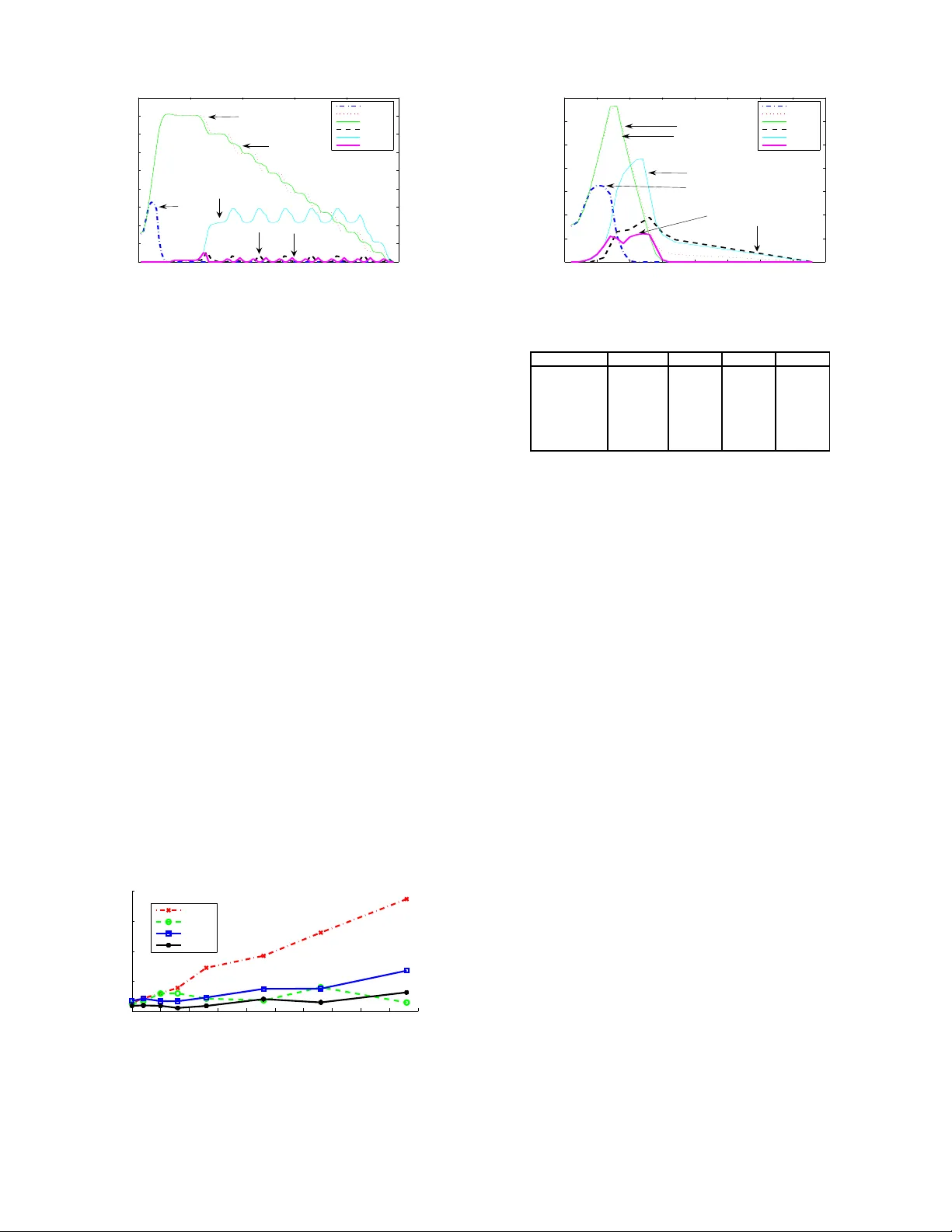
1 Subspace Properties of Ne tw ork Coding and their Applic ations M. Jafari Sia v oshani, Student Member , I EEE , C. Fragouli, Member , IEEE , S . N. Digga vi, Member , IEEE Abstract —Systems that employ netwo rk coding f or content distribution conv ey to the receiv ers linear combinations of the source packets. If we assume randomized network coding, d uring this process the network nodes collect random subspaces of the space sp anned by the source packets. W e establi sh severa l fundamental properties of the random subspaces induced in such a system, and show that these subspaces implicitly carry topological informa tion about the network and its state that can be passiv ely collected and inferred. W e lever age t his information towards a n umber of app lications that are interesting in their own right, such as topology i nference, bottleneck di scov ery in peer -to-peer systems and locating Byzantine attackers. W e thu s argue that, randomized network coding, apart from its b etter known properties for impro ving information delivery rate, can additionally facilitate network management and control. I . I N T R O D U C T I O N Randomized network cod ing offers a prom ising tec hnique for co ntent distribution systems. I n r andomized network cod- ing, each node in the network comb ines its incom ing pa ckets random ly and sends them to its neig hbour s [ 1], [2]. Th is is the approach adopted by mo st practical app lications today . For examp le, A v alan che, th e ﬁrst impleme ntation o f a peer- to-peer (P2 P) system th at uses network codin g, adopts su ch a random ized op eration [3], [4]. In ad-ho c wireless an d sensor networks as we ll, most prop osed protocols employing network coding again opt for rand omized network operatio n (see [9] and r eferences therein ). The reason for the popular ity of random ized network coding is because it facilitates a very simple and ﬂexible network operation without need o f syn chronizatio n am ong n etwork nodes, tha t is well suited to pac ket networks. T o every packet, a coding vector is appen ded that de termines how the packet is expressed with respect to th e orig inal data packets pr oduced at the source n ode. When interm ediate n odes combine packets, the coding vector keep s track of the linear co mbinations contained in a pa rticular packet. A rece i ver which collects enoug h packets, uses the coding vectors to determin e th e set of linea r e quations it ne eds to solve in order to recover the original data pa ckets. The work of M. Jafari S ia vosha ni and C. Fragouli was supported by the Swiss Nationa l Science Foundat ion through Grant PP00P2-128639. M. Jafari Siav oshani and C. Fragouli are with the School of Computer and Communicat ion Sciences, Ecole Polytechnique F ´ ed ´ erale de Lausanne (EPF L), Lausanne CH 1015, Switzerland (e-mail: m ahdi.ja fari siav oshani@ep.ch; christin a.fragouli @ep.ch). S. N. Digga vi was with the Ecole Polytec hnique F ´ ed ´ erale de Lausanne (EPFL), Lausanne CH 1015, Switzerland. He is now with the Department of Electric al Engineering, Univ ersity of California , Los Angeles (UCLA), CA 90095 USA (e-mail: suhas@ee.ucla .edu). Our con tributions start with the observation that cod ing vec- tors imp licitly carry inf ormation abo ut the n etwork struc ture as well as its state 1 . Su ch vectors b elong to appro priately deﬁned vector spaces, an d we ar e interested in funda mental proper ties of these (ﬁnite-ﬁeld) vector spaces. In particular, since we ar e in vestigating prop erties ind uced by random ized network codin g, we need to c haracterize ran dom subsp aces of the afo remention ed vector spaces. These proper ties of rando m subspaces over ﬁnite ﬁelds migh t be o f indep endent interest. W e aim to show , using these prop erties, that observing the coding vectors we c an passiv ely collect struc tural and state informa tion about a network. W e can lev erage this infor mation tow a rds sev e ral application s that are interesting in their own merit, su ch as topolo gy infere nce, network tomog raphy , an d network managemen t (we do n ot claim here th e design of practical p rotocols th at use these pro perties). Howe ver , we show th at ran domized network coding, apart fro m its b etter known pr operties f or facilitating infor mation de li very , can provide us with inf ormation abou t the ne twork itself. T o suppor t this claim, we start by studying the problem of passi ve topology inference in a content distrib ution sys- tem where interm ediate nodes perfor m rand omized network coding. W e show th at the subsp aces no des co llect d uring th e dissemination p rocess h a ve a depe ndence with each other which is in herited fr om the network structure. Using th is depend ence, we d escribe the cond itions that let u s perfectly reconstruc t the topology of a network, if subspaces of all nodes at som e time instant are available. W e then in vestigate a r e verse or dual pro blem of top ology inference , which is , ﬁnding the location of Byzantine attackers. In a network coded system, the adversarial no des in the network can disrup t the n ormal o peration of info rmation ﬂow by inserting erroneo us p ackets into the n etwork. W e u se the depend ence between s ubspaces gathered by network nodes and the to pology o f the network to extract info rmation abou t the location of attackers. W e pr opose several method s, co mpare them and inves tigate th e condition s that allow us to ﬁnd the location of attackers u p to a small un certainty . Finally , we then observe that the r eceiv ed su bspaces, e ven at one speciﬁc node, re veal so me information about th e network, such as the existence of bo ttlenecks or congestion . W e conside r P2 P n etworks for con tent distribution that use random ized n etwork coding techniqu es. It is known that th e perfor mance of such P2P networks depen ds critically on the good con nectivity of th e overlay to pology . Building on our 1 By state we refer to link or node failures, congestion in some part of the netw ork, etc. 2 observation, we p ropose algo rithms fo r topolog y manage ment to avoid bottlenec ks and clusterin g in network-cod ed P2P systems. T he pro posed approac h is decentralized , inhe rently adapts to the network to pology , and redu ces substantially the number of topo logy rewirings th at are necessary to ma intain a well connected o verlay ; moreover , it is integrated in the normal content distribution. The paper is organized as follows. W e star t with the notation and pro blem modelin g in § II. W e in vestigate the pro perties of vector spaces in a system that emp loys r andomized ne twork coding in § III and these pro perties give th e framework to explore application s in § IV, § V, and § VI. Finally , we conclu de the paper with a discussion in § VII. Sho rter versions of the se results h av e also appeare d in [10], [11], [1 2]. A. Related W ork Network co ding started by the work o f Ahlswede et al. [13] who showed that a so urce can multica st in formation at a rate app roaching the smallest m in-cut between the source and any rec ei ver if th e middle nod es in th e network combin e the infor mation packets. Li et al. [ 14] showed that linear network coding with ﬁnite ﬁeld size is sufﬁcient for multicast. K o etter et al. [ 15] presented an algeb raic f ramew ork fo r linear network codin g. Randomized network coding was propo sed by Ho et al. [16] where they showed that ra ndomly ch oosing th e n etwork code leads to a valid solution for a multicast problem with high probab ility if the ﬁeld size is large. I t was later app lied by Chou e t a l. [2] to demo nstrate th e p ractical aspects of rand om linear network cod ing. Gkan tsidis et al. [3], [4] imp lemented a practical ﬁle sharing system based on th is idea. Several other works ha ve also adopted randomized network codin g for co ntent distribution, see for examp le [5 ], [6], [7]. Network err or co rrecting co des, that are capable of cor rect- ing errors inserted in th e network , have been developed during the last few y ears. For exam ple see the work of K oetter et al. [17], Jaggi et al. [18], Ho et al. [19], Y eung et al. [20], [21], Zhang [2 2], an d Silva et al. [23]. These sch emes ar e cap able of delivering info rmation despite the pr esence of Byzantine attacks in the network or no des m alfunction , as lon g as the amount of undesired inf ormation is limited . T hese network error correctin g schemes allow to cor rect maliciou s packet corrup tion up to certain rate. In contrast, we use n etwork coding to identif y maliciou s nod es in ou r work. Recently , and following o ur work [12], ad ditional ap proaches are pro posed in th e literature, some building o n our results [24]. Overlay topo logy mon itoring an d m anagemen t that do not employ network cod ing has been an intensi vely stud ied re- search top ic, see for example [25]. Howe ver, in th e co ntext of network coding , it is a new area of research. Fragou li et al. [26], [27] took advantage of network coding capabilities for activ e link lo ss network m onitoring whe re the focus was on link lo ss rate inference. Passi ve infere nce of link loss rates has also been pro posed by Ho et al. [28]. In a subseq uent work of ours, Sharm a et a l. [ 29] stud y passiv e to pology estimation f or the u pstream no des of every network node. This work is based on th e assumption th at the lo cal codin g vectors for eac h nod e in the network ar e ﬁxed, generated in advance and known by all other nod es in th e network, u nlike ou r work that builds on rand omized operation. The idea of passive infe rence of topolog ical properties from su bspaces th at ar e build over time, as far as we know , is a novel contribution of th is work. I I . M O D E L S : C O D I N G A N D N E T W O R K O P E R A T I O N A simple observation motivates much of th e work presented in this paper: th e subspaces gathere d by the network no des during in formation disseminatio n with r andomized n etwork coding, ar e not co mpletely rand om, but h av e some rela- tionship, and this r elationship co n veys info rmation abo ut the network to pology as well as its state. W e will thu s investigate proper ties o f the collected subspa ces and show how we can use th em for d i verse application s. Different p roperties o f the subspaces are relev ant to e ach particular application and ther efore we will develop a fr ame- work for inv estigating these prop erties. This will also inv o lve some understandin g of modeling the p roblem to ﬁt the re- quiremen ts of an application an d then de velop ing subspace proper ties relevant to that mo del. A. Notation Let q ≥ 2 be a power of a p rime. In th is pape r , all vectors and matrices have elem ents in a ﬁnite ﬁeld F q . W e use F n × m q to denote the set of all n × m matrices over F q , and F ℓ q to denote the set of all row vectors of leng th ℓ . The set F ℓ q forms an ℓ -d imensional vector space over the ﬁeld F q . Note that all vectors are r ow vectors unless otherwise stated. Bold lower - case letters, e.g. , v , are used for vectors and bold capital letters, e.g. , X , are used to d enote matr ices. For a set of v e ctors { v 1 , . . . , v k } we denote their linear span by h v 1 , . . . , v k i . For a matrix X , h X i is the subspac e spanned by the rows of X . W e then h av e r ank( X ) = dim( h X i ) . W e denote subspaces of a vector space b y Π and some times also b y π . In this paper, we work on a vecto r space F ℓ q of dimension ℓ deﬁned over a ﬁnite ﬁeld F q . For two subspaces Π 1 , Π 2 ⊆ F ℓ q , we will denote their intersection b y Π 1 ∩ Π 2 and th eir joint sp an b y Π 1 + Π 2 where Π 1 + Π 2 , { v 1 + v 2 | v 1 ∈ Π 1 , v 2 ∈ Π 2 } , is the smallest sub space tha t contain s b oth Π 1 and Π 2 . It is well k nown that dim(Π 1 + Π 2 ) = dim(Π 1 ) + dim(Π 2 ) − dim(Π 1 ∩ Π 2 ) . W e also use the f ollowing metric to measu re th e distance between two subspaces, d S (Π 1 , Π 2 ) , dim(Π 1 + Π 2 ) − dim(Π 1 ∩ Π 2 ) (1) = dim(Π 1 ) + dim(Π 2 ) − 2 dim(Π 1 ∩ Π 2 ) . This metric was also introdu ced in [1 7], where it was used to design er ror corre ction codes. In a ddition to the metric d S ( · , · ) d eﬁned a bove, in some cases we will also need a m easure that compa res how a set A 3 of subspaces differs from anoth er set B of su bspaces. For this we will use th e average pair-wise distance deﬁned as follows D S ( A , B ) , 1 |A||B | X π a ∈A ,π b ∈B d S ( π a , π b ) . (2) It shou ld be no ted that the above relatio n do es not d eﬁne a metric fo r th e set of subspaces because th e self distance of a set with itself is no t zero. Howe ver, D S ( · , · ) satisﬁes the triangle in equality . In this pap er we will b e interested in investigating the relationship of the collected subspaces at neig hborin g network nodes. W e consider a n etwork represented as a directed acyclic graph G = ( V , E ) , with ϑ = | V | no des and ξ = | E | edges. For an a rbitrary edge e = ( u, v ) ∈ E , we d enote head( e ) = v and tail( e ) = u . For an arbitrary n ode v ∈ V , we den ote In( v ) th e set of incoming edg es to v and Out( v ) th e set of outgoin g edg es fro m v . If a nod e u has p parents u 1 , . . . , u p , we d enote with P ( u ) = { u 1 , . . . , u p } the set of p arents of u . W e use P l ( u ) to d enote the set of all ance stors of u at distance l from u in th e network (we say that two n odes u an d v are at distance l if there exists a path of length exactly l that connects them). W e d enote with π ( u i ) u ( t ) the sub space no de u receives f rom pa rent u i at exactly time t , an d with π u ( t ) the whole subspace (fr om all p arents) that node u rece i ves at time t , th at is π u ( t ) = P p i =1 π ( u i ) u ( t ) . W e also den ote with Π ( u i ) u ( t ) the subspace node u has received from p arent u i up to time t , that is, Π ( u i ) u ( t ) = Π ( u i ) u ( t − 1) + π ( u i ) u ( t ) . T hen the subspace Π u ( t ) th at the n ode has at time t can be expr essed as Π u ( t ) = P p i =1 Π ( u i ) u ( t ) . For a set of nod es U = { u 1 , . . . , u p } , we d eﬁne Π U = Π u 1 + · · · + Π u p . Finally , we use the big O notation which is deﬁned as follows. Let f ( x ) and g ( x ) be two fu nctions deﬁned on some subset of the real number s. W e write f ( x ) = O ( g ( x )) if and on ly if there exists a po siti ve re al nu mber M and a real number x 0 such that | f ( x ) | ≤ M | g ( x ) | f or all x > x 0 . Dur ing the rest of the paper we use O to comp are func tions of the ﬁeld size q , unless otherwise stated. For example, we will use f ( q ) = O ( q − 1 ) to imply that th e value o f f ( q ) goes to zero as q − 1 for q → ∞ . B. Network Operation W e assum e that th ere is an in formation sourc e lo cated on a node S that h as a set of n packets (messages) { x 1 , . . . , x n } , x i ∈ F ℓ q , to distribute to a set of receivers, where each packet is a sequen ce of ℓ sym bols over the ﬁn ite ﬁeld F q . T o do so, we will emp loy a dissemination p rotocol b ased on random ized network coding, namely , where each network node sends rando m linear comb inations (chosen to be unif orm over F q ) of its collected p ackets to its neighbo rs. W e assume for simplicity that ther e are n o packet-losses. Dissemination P r otocol It is p ossible to separate the dissemination protoc ols into the following oper ation categories. • Synchr on ous: All nodes are syn chronized and tran smit to their n eighbors accord ing to a glo bal clock tick (time- slot). At timeslot t ∈ N , nod e v sends linear com binations from a ll vecto rs it has collec ted up to tim e t − 1 . Once nodes start tran smitting info rmation, they keep transmit- ting un til all r eceiv ers are ab le to decod e. • Asynchr ono us: Nodes transmit lin ear combinatio ns at random ly and indepe ndently cho sen time instants. In this pape r , we focus o n the synch ronous network where we assume that each link has unit delay 2 correspo nding to each timeslot, h owe ver our results can b e extended to asynchro nous networks as well. Next, we explain in d etail the disseminatio n proto col, that is summ arized in Algorithm II.1. T im ing: W e depict in Fig. 1 the relative timing o f ev ents within a timeslot. Nod es transmit at the beginning of a time slot. W e assume that each packet is re cei ved by its intended receiv er b efore the end of th e timeslot. Thus, the timeslot duration incorpo rates the pa cket prop agation delay in one ed ge of the ne twork. Time t − 1 t Slot number t A B A Transmits B R eceives n The point that subspa ces are mea sured: Π B ( t ) Π A ( t − 1) Fig. 1. Timi ng schedule of the disseminat ion protocol gi ven by Algo- rithm II.1. Rate Allocatio n and Equiva lent Network Grap h: The dissemination protoco l ﬁrst associates with each link e of the network a rate r e (measured as th e number of p ackets transmitted per timeslot o n edge e ). Th ese rates are selected in advance using a r ate allo cation method , fo r example [8]. For the rest of the p aper, we con sider an equ i valent network graph, where each edge e has cap acity eq ual to its allo cated rate r e . On this new graph, we can d eﬁne the min-cu t c v from the source no de S to a n ode v ∈ V . Whenever we ref er to min-cut values in the f ollowing, we imply min -cut values over this eq uiv alent gr aph. W e assume that the rate allocation pro tocol we u se satisﬁes r e ≤ min[ c e , c tail( e ) ] , (3) where c e is the ca pacity of edg e e . This very mild assumption says that the nod e v = tail( e ) do es not sen d more infor mation than it receives, and is satisﬁed by all pro tocols that do no t send red undant packets, i.e. , o bserve ﬂow co nservation. In our work, we consider the case w here n ≫ c v , namely , the dissemination of the n so urce packets to the receivers takes place by using the network over se veral timeslots. Node op eration: When the dissemination starts, at times- lot say z ero, the source starts transmitting at each time slot and to each of its outg oing edges e , r e random ly selected linear comb inations of n inform ation p ackets. W e will call r S the source rate . The source con tinues un til it has transmitted linear combinations of all n p ackets, i.e. , f or n r S timeslots. 2 Unit delay can model a buffe ring windo w a node needs to wait to collec t pack ets from all its neighbors. 4 Every oth er nod e v ∈ V \ { S } in the network, operates as follows: • Initially it d oes not transmit, but only collects in a buffer packets fr om its parents, until a time τ v , which we call waiting time and we will deﬁne in the following. As we will see, each nod e can decid e the waiting time by itself and in dependen tly from other no des. • At each timeslot t , f or all t ≥ τ v + 1 , it tra nsmits to ea ch outgoin g edg e e , r e linear co mbinations of all packets it has c ollected in its buffer up to time t − 1 . Collected Subspaces: W e can think of each o f the n source m essages { x i } as co rrespond ing to one dimension of an n -dimensio nal sp ace Π S ⊆ F ℓ q where Π S = h x 1 , . . . , x n i . W e say that node v ∈ V at time t observes a subspace Π v ( t ) ⊆ Π S , with dimension d v ( t ) , dim(Π v ( t )) , if Π v ( t ) is th e space spanned by the received v ectors at node v up to time t . Initially , at time t = 0 , the collected sub spaces o f all nod es (ap art th e source) are emp ty; d v (0) = 0 , ∀ v ∈ V \ { S } . W aiting Ti mes: W e next d eﬁne the waiting times, that will b e used in the f ollowing sectio ns to en sure th at th e subspaces o f different no des be distinct, and are a usual assumption in disseminatio n p rotocols; in deed, for large n the waiting time does not affect th e rate. For exam ple, in the informa tion-theor etic proof of the main theorem in network coding [13], ea ch nod e waits u ntil it collects at least on e message from each of its incomin g links b efore starting transmissions. Deﬁnition 1: The waiting time τ v for a no de v is the ﬁrst timeslot during which nod e v r eceiv es infor mation fro m the source at a rate equ al to its min- cut c v , and add itionally , has collected in its buffer a sub space of dimension at lea st c v + 1 . Note that, because we are dealing with acyclic gr aphs, we can imp ose a par tial order o n th e waiting times of the no des, such that all p arents o f a node have smaller waiting tim e than th e node. Moreover, each no de can decid e whether the condition s f or the waiting time are met, by obser ving wheth er it receives in formation at a r ate eq ual to its min-cu t, and what is the dimension of the subspace it has co llected. That is, a no de d oes not need to know any top ological infor mation (apart fro m its min- cut), a nd the waiting times d o no t ne ed to be commu nicated in advance to the node s, but can be decid ed online b ased on the n etwork cond itions. Algorithm II.1: D I S S E M I N A T I O N P ROT O C O L ( G = ( V , E ) , S, n, τ v , r e ) for ea ch v ∈ V \ { S } do Π v (0) = ∅ , d v (0) = 0 t ← 1 while min v d v ( t ) < n                        for ea ch v ∈ V        if t ≥ τ v + 1 then    for ea ch e ∈ Out( v ) do  node v transmits fro m Π v ( t − 1) with r ate r e on e for ea ch v ∈ V do up date Π v ( t ) , d v ( t ) t ← t + 1 Alg. II. 1: Dissemination proto col. Source Operation and the Source Subsp ace Π S As we discussed, th e source needs to convey to the receivers n so urce pac kets th at span th e n -dim ensional subspace Π S = h x 1 , . . . , x n i , with Π S ⊆ F ℓ q . Π S is iso morphic to F n q ; thus, for the purpo se of study ing r elationships b etween su bspaces of Π S , we can eq uiv alently assume that Π S = F n q , and that node v ∈ V at time t ob serves a sub space Π v ( t ) ⊆ Π S . T his simpliﬁcation is very natural in the ca se where we employ coding vectors, reviewed b rieﬂy in the f ollowing, as we only need consid er the c oding vectors f or our purp oses and ignore the remainin g conten ts of the pa ckets; however , we can also use th e same ap proach in th e case where th e sou rce per forms nonco herent codin g, described sub sequently . a) Use o f Coding V ectors: T o enable receivers to decode, the source assigns n symbols of ea ch message vector (packet) to determine the linear re lation be tween that packet and the original vectors x i , i = 1 , . . . , n . W ithou t loss of generality , let us assume these n symb ols ( which form a vector of length n ) are placed at the beginning of each message vector . This v ector is called codin g vector . Each m essage vecto r x i contains two parts. Th e vector x C i ∈ F n q with length n is the cod ing vector and remain ing part, x I i ∈ F ℓ − n q , is the inform ation p art where x i , [ x C i | x I i ] . The cod ing vectors x C i , i = 1 , . . . , n are chosen such that they form a b asis fo r F n q . For simplicity we assume x C i = e i where e i ∈ F n q is a vector with on e at p osition i an d zero elsewhere. For our pur poses, it is sufﬁcient to restrict o ur algorith ms to examine th e codin g vectors. Thus, the sou rce has the space Π S = F n q ; during the informatio n d issemination, if a node v at time t has collected m packets z i with coding vectors z C i , it ha s observed the subspace Π v ( t ) =  z C 1 , . . . , z C m  . In other words, the co ding vectors capture all the inform ation we need for o ur application s. b) Subsp ace Cod ing: Our approach also works in the case of sub space cod ing, that was introdu ced in [ 17]. W e next brieﬂy explain the idea o f comm unication using sub spaces, in a n etwork p erformin g rand omized network codin g. In the following, we use th e same n otation as introduc ed in § II-B. Let { x 1 , . . . , x n } , x i ∈ F ℓ q denote the set of 5 packets the sou rce h as. Assume tha t th ere is no er ror in the network . An arbitrary receiver R v at nod e v collects m packets z i , i = 1 , . . . , m , whe re each z i can b e pr esented as z i = P n j =1 h ij x j . The coefﬁcients h ij are unkn own and random ly chosen over F q . In matr ix form, the transm ission model c an be represented a s Z v = H S v X , where H S v ∈ F m × n q is a rando m matr ix and X ∈ F n × ℓ q is the matrix whose rows are the sou rces’ packets. The matrices H S v are random ly c hosen, u nder constra ints imposed by the network topology . As stated in [17] and proved in [30], [31], [32], the ab ove model n aturally leads to con sider informa tion tr ansmission n ot via the ch oice o f x i but rather by the ch oice of the vector spac e span ned by { x i } . In the case of subspace c oding, the dissemination algor ithm works in e x actly the same way as in the case of coding v ectors; what c hanges is how the source m aps the inform ation to th e packets it transmits, and ho w decoding occurs. Howe ver, th is is orthog onal to our purp oses, since we p erform no decodin g o f the info rmation m essages, but simply observe th e relationsh ip between the subspa ces different nodes in the network collect. Thus, th e same appro ach can be applied in this case as well. C. In put to Algorithms W e ar e interested in design ing algorithm s that lev erage the relationships b etween subspaces ob served at different n etwork nodes for n etwork man agement and con trol. Th e a lgorithms design will depen d on th e in formation that we have access to. W e distinguish betwe en the f ollowing. • Global in formation : A central e ntity knows the sub spaces that all ϑ nod es in the network h av e observed. • Local Informatio n: There is no such omn iscient en tity , and each nod e v only knows what it has re cei ved, its own sub space Π v . W e may also have in formation between these two extreme cases. Mor eover , we may have a static view , wh ere we take a snapsho t of th e network at a given tim e instant t , or a no n- static view , where we take several snapshots of th e n etwork and u se the subspaces’ ev olutio n to d esign an algorithm . W e will argu e in Section I V that capturing even glob al informa tion can be accom plished with relatively low overhead (sending o ne add itional packet per n ode at th e en d of the dissemination proto col); thus, the algorithm s we develop even assuming global info rmation can in fact be implemented almost passively an d at low cost. I I I . P R O P E RT I E S O F R A N D O M V E C T O R S PAC E S O V E R A F I N I T E F I E L D F n q In this section, we will state a nd pr ove b asic prop erties and results th at we will exploit towards various applicatio ns in the following sections. In particu lar , we will inv e stigate the prop erties o f rando m sampling from vector spaces over a ﬁnite ﬁeld. Such prop erties give us a better insight and understan ding of r andomized network codin g and form a found ation for the results a nd algo rithms pre sented in this paper . A. Sa mpling S ubspaces over F n q Here, we explore prop erties of rando mly sampled subspaces from a vector sp ace F n q . W e start with the following lemma that explore s pro perties of a single subsp ace. Lemma 1: Suppo se we choose m vectors f rom an n - dimensiona l vector space Π S = F n q unifor mly at random to construct a space Π . Then the subspace Π will be full rank (has dimension min[ m, n ] ) w . h.p. (with h igh prob ability) 3 , nam ely , P [dim(Π) = min [ m, n ]] = [1 − O  q − 1  ] . Pr oof: Refer to App endix A. W e con clude that f or large values o f q , selecting m ≤ n vectors unif ormly at r andom fr om F n q to construct a subspa ce Π is equivalent to ch oosing an m -dimen sional subspace fro m F n q unifor mly at rand om. Note that this is not true f or sma ll values o f q . W e next examine con nections between multiple subspaces. Lemma 2: Let Π 1 and Π 2 be two sub spaces of Π S = F n q with d imension d 1 and d 2 respectively , inter section of di- mension d 12 and Π 1 * Π 2 ( i.e. , d 12 < d 1 ). Con struct Π ′ 1 by cho osing m vectors fro m Π 1 unifor mly at rando m. Then P [Π ′ 1 ⊂ Π 2 ] = O ( q − m ) . Pr oof: Refer to App endix A. Lemma 3: Suppo se Π k is a k -dimension al subspace o f a vector space Π S = F n q . Select m vectors u niformly at r andom from Π S to con struct the su bspace Π . W e have dim(Π ∩ Π k ) = min[ k , ( m − ( n − k )) + ] = (min[ m, n ] + k − n ) + , (4) with pro bability 1 − O  q − 1  . Pr oof: Refer to App endix A. Corollary 1: Suppo se Π 1 and Π 2 are two subspace of F n q with dimensio n d 1 and d 2 respectively an d joint dim ension d 12 . Let us take m 1 vectors u niformly at r andom from Π 1 and m 2 vectors fr om Π 2 to construc t subspac es ˆ Π 1 and ˆ Π 2 . W e h a ve dim( ˆ Π 1 ∩ ˆ Π 2 ) = min  d 12 , ( m 1 + m 2 − ( d 1 + d 2 − d 12 )) + , ( m 1 − ( d 1 − d 12 )) + , ( m 2 − ( d 2 − d 12 )) +  , with pro bability 1 − O  q − 1  . Pr oof: Refer to App endix A. By choosing Π 1 = Π 2 = F n q in Corollary 1 we h a ve the following co rollary . Corollary 2: Let u s construc t two subspaces ˆ Π 1 and ˆ Π 2 by choosing m 1 and m 2 vectors uniformly at random respectively from F n q . Then th e subspaces ˆ Π 1 and ˆ Π 2 will be d isjoint with probab ility 1 − O  q − 1  if m 1 + m 2 ≤ n . W e are n ow ready to d iscuss one of the imp ortant prop erties of ran domly ch osen subspa ces which is very useful for o ur work: ran domly selected subspaces tend to be “as far as possible”. W e will clarify an d make precise what we mean by “as far as possible”, see also [33]. W e ﬁr st review the 3 Throughout this paper , when we talk about an eve nt occurring with high probabil ity , we m ean that its probabil ity behav es lik e 1 − O  q − 1  , which goes to 1 as q → ∞ . 6 deﬁnition of a sub space in genera l po sition with resp ect to a family of subspaces. Deﬁnition 2 ([33, Chapter 3]): Let Π S be an n - dimensiona l space over the ﬁeld F q and fo r i = 1 , . . . , r , le t Π i be a subspace o f Π S , with dim(Π i ) = d i . A subspace Π ⊆ Π S of dimension d is in gen eral position with r espect to the family { Π i } if dim(Π i ∩ Π) = ma x [ d i + d − n, 0 ] , ∀ i ∈ { 1 , . . . , r } . (5) It should be no ted th at max[ d i + d − n, 0] is the minim um possible dim ension of (Π i ∩ Π) . So what the above deﬁnition says is that the intersection o f Π and each Π i is a s sma ll as possible. Using the ab ove deﬁnition we can state the following theorem 4 . Theorem 1 : Suppo se { Π i } , i = 1 , . . . , r , are sub spaces of Π S = F n q . Let us con struct a subsp ace Π by rando mly choosing m vectors from Π S . Then Π will be in gen eral position with resp ect to the family { Π i } w .h .p., i.e. , with probab ility 1 − O  q − 1  . Pr oof: Refer to App endix A. Theorem 1 d emonstrates a n ice pro perty of rando mized net- work c oding where the subspaces spann ed by coding vectors tend to be as far a s po ssible o n different paths of the n etwork. B. Rate of Innovative P ackets In the following sections, we will nee d to know the rate of receiving innovati ve message vectors (p ackets) at receivers in a dissemination protoc ol per forming rand omized network coding. By innovati ve we refer to vectors that do not b elong in the space sp anned by alr eady collected p ackets. As it is shown in [1 3], the source can multicast at ra te eq ual to the minimum min- cut of all receivers if the in termediate nodes can com bine th e incom ing me ssages. Mo reover , it is shown in [14] that u sing linear combin ations is sufﬁcient to achieve informa tion tran sfer at a rate eq ual to the minimum mincut of all r eceiv ers. In [13], [1], it is also demonstrated that choosing the coefﬁcients of the linear comb inations r andomly is sufﬁcient (no network -speciﬁc code d esign is requir ed) with high p robability if the ﬁeld size is large enou gh. T o ﬁnd the rate o f rece i ving inform ation at each no de where the implemen ted dissemination proto col perfo rms rando mized network cod ing, we can use the following result given in Theorem 2 . No te th at our d escribed d issemination p rotocol, although very c ommon in practice, does not exactly ﬁt to the pr evious the oretical results in the literatur e that examin e rates, bec ause the operation of th e network no des is not memory -less. That is, while for example in [1], [13], [14] each transmitted packet a t time t is a f unction of a small subset of the recei ved packets up to time t (the ones correspon ding to th e same infor mation message), in ou r case a pac ket transmitted at time t is a rando m lin ear c ombination of all packets re cei ved up to time t . This small variant o f the main theo rem on random ized network co ding is very intu iti ve, a nd we formally state it in following. 4 V ersions of this theorem can be easily deriv ed from results in the literature [33], but we repeat here the short deri vation for completeness Theorem 2 : Consider a source that transmits n packets over a con nected network using th e dissemination protocol described in § II-B, and assume that the network nod es perform random linear network coding over a sufﬁciently large ﬁnite ﬁeld. T hen ther e exists t 0 such that for all t > t 0 each node v in the network receives c v indepen dent linear c ombination s of the n source p ackets per time slot, wher e c v = mincut ( v ) . Pr oof: Refer to App endix B-A. Giv e n T heorem 2, we can state th e following deﬁnition. Deﬁnition 3: For a speciﬁc inf ormation d issemination pro- tocol over a network, we deﬁne the stead y state a s the time period du ring which each no de v in the network receives exactly c v indepen dent linear co mbinations of the n source packets p er tim e slot and none of the n odes, except sour ce S , has collected n line arly ind ependen t combinatio ns. W e call the time that the network en ters steady state p hase th e steady state starting time and de note it by T s . If the n etwork never attains th e steady state phase then we use T s = ∞ . For ou r pr otocol in § II-B, T s depend s n ot o nly on the network to pology , but also on the waiting times τ v . For the waiting time deﬁned in Deﬁnition 1 w e can upp er bou nd T s as stated in Lemma 4 . Lemma 4: If n is large enoug h, for the disseminatio n protoco l given in § I I-B we may upp er b ound the steady state starting time as follows T s ≤ 2 D ( G ) − 1 , where D ( G ) is the longest path fr om the sou rce to oth er nodes in the network 5 . Pr oof: Refer to App endix A. In or der to b e sure that the disseminatio n pro tocol given in § II-B enters th e steady state phase, n should b e large enoug h. Using Lem ma 4 we have the following result, Coro llary 3. Corollary 3: A sufﬁcient cond ition for n to be sure that the protoco l en ters the steady state is that 2 D ( G ) − 1 < ⌊ n c max ⌋ , where c max = max v ∈ V c v . I V . T O P O L O G Y I N F E R E N C E In th is section, we w ill use the too ls d e veloped in § III to in vestigate the relation between th e ne twork to pology an d the subspaces collec ted at the n odes during in formation dissemi- nation. W e will develop condition s that allow us to p assi vely infer the network topo logy with ( asymptotically on the value of q ) no error . Th e propo sed schem e is passiv e in the sense that it do es n ot alter the normal da ta ﬂow of the network, and the in formation rates that can be achiev ed. In fact, we can think of o ur p rotocol as identify ing the top ology of th e network which is ind uced by the trafﬁc. W e build our intuition starting from inf ormation d issem- ination in tree to pologies, and then extend ou r results in arbitrary topologies. Note that inform ation dissemination using network c oding in tree topolo gies doe s no t o ffer throug hput 5 Note that D ( G ) is differen t from the longest shortest path which is calle d diamete r of G in the graph theory literature . 7 beneﬁts as comp ared to routing ; howev er , it is an inter esting case study that will natu rally lead to our fra mew o rk for general top ologies. W e then deﬁne cond itions under which the top ology of a tree and that of an arb itrary network can be uniquely ide ntiﬁed using the obser ved subspaces. Note that uniquely id entifying the topolog y is a strong req uirement, as the num ber of topo logies for a given number of network nodes is expon ential in the num ber of n odes. A. T r ee T op ologies Let G = ( V , E ) be a network that is a directed tree of depth D ( G ) , rooted at the source nod e S . W e will present (i) ne cessary and sufﬁcient cond itions under which th e tree topolog y ca n be uniquely identiﬁed, and (ii) given that these condition s are satisﬁed, a lgorithms th at allow us to do so. W e ﬁrst con sider trees where each edge is allocated the same rate c , and thus the min- cut from the source to each node of th e tree equals c . W e then brieﬂy discuss the case of undir ected trees. Finally we examin e the case where edges are allocated different rates, and thu s nodes ma y have different min-cuts f rom the source. 1) Commo n Min-Cut: Assume th at ea ch edge of the tree has the same capacity c ( i.e. , a rate alloca tion alg orithm h as assigned the same r ate r e = c on each edge of th e tree). Thus all no des in the tree h av e the same min -cut, equal to c . Then according to the disseminatio n pr otocol intr oduced in Algor ithm II.1, each no de v will wait time τ v , until it has collected a c + 1 dimensional subspace, an d then start transmitting to its ch ildren. Our claim is that, we can then identify the n etwork top ology using a single snapsho t of all node’ s subspaces at a time t . Before forma lly proving the result in T heorem 3, we will give some intuition on why this is so, and wh y the waiting time is c rucial to achieve this. W e star t from an example o n the simple n etwork in Fig ure 2. Example 1: Consider the tree in Figure 2 and assum e that the edg es have u nit capacity ( c = 1 ). Alg orithm II.1 works as fo llows . At tim e t = 1 , node A receiv es a vector y 1 from the source S . Node A waits, as it h as not yet collected a c + 1 = 2 dim ensional sub space. At time t = 2 , it re cei ves a vector y 2 . It now has collected the subspace Π A (2) = h y 1 , y 2 i , and thus at th e next timeslot it will start transm itting. At tim e t = 3 , node A transmits vector s y B 1 and y C 1 to n odes B and C respectiv ely , with y B 1 , y C 1 ∈ Π A (2) . Thus Π B (3) =  y B 1  and Π C (3) =  y C 1  . Nod e A also r eceiv es a vector y 3 from the so urce, and th us Π A (3) = h y 1 , y 2 , y 3 i . Consider n ow the subspaces Π A (3) , Π B (3) a nd Π C (3) . W e see that Π B (3) ⊆ Π A (3) , an d Π C (3) ⊆ Π A (3) ; we thus co nclude that n odes B and C are children of nod e A . Mo reover , Π B (3) 6 = Π C (3) , which will allow us to d istinguish betwe en ch ildren o f these two nod es when we deal with larger tr ees. In contr ast, if Algo rithm I I.1 did not imp ose a waiting time, and node A started transmitting to no des B and C at tim e t = 2 , then both no des B and C would receive the same vector y 1 , i. e. , Π B (2) = Π C (2) = h y 1 i . In fact, at a ll subseq uent times, we will have that Π B ( t ) = Π C ( t ) = Π A ( t − 1 ) . Thus, we would no t be able to distinguish between these two no des.  S Π S A Π A ( t ) B Π B ( t ) C Π C ( t ) π A ( t ) π B ( t ) π C ( t ) Fig. 2. Directed tree with four nodes rooted at the source S . The main idea in our r esult is th at, if we c onsider two nodes u and v at the network which have collected su bspaces Π u ( t ) and Π v ( t ) at time t , then, u nless u an d v h av e a child -ancestor relationship ( i. e. , are on the sam e b ranch in th e tre e), it h olds that Π u ( t ) * Π v ( t ) and Π v ( t ) * Π u ( t ) . The challen ge in proving this is th at we dea l with subspaces ev olvin g over time , and thus we cann ot directly apply th e results in § II I. For example, fo r the ne twork in Figure 2, Π B ( t ) and Π C ( t ) are not subspaces that are selected uniformly at rand om fr om Π A ( t ) ; instead, th ey are build over time as Π A ( t ) a lso ev olves. W e will thu s need the following two results, that m odify the r esults in § I II to take into accoun t the time ev olution in the creation of th e subspaces. W e start by exam ining in Lem ma 5 the r elationship betwe en subspaces collected at the immediate c hildren o f a given parent node (for example, at the child ren B and C of node A ). These are created by samp ling the sam e subspaces (those at n ode A ). W e th en examine in Coro llary 4 the re lationship b etween subspaces collected at nodes that have different parents (for example, a node that h as B as pare nt an d a nod e th at has C as pa rent). Lemma 5: Suppo se there exist (pro per) subspace s Π(0) ⊂ Π(1) ⊂ · · · ⊂ Π( t − 1 ) with dimensions d 0 , . . . , d t − 1 , respectively . Let us co nstruct the set of subspac es Π u ( i ) , i = 1 , . . . , t , as follows. Set Π u ( i ) = P i j =1 π u ( j ) where π u ( j ) is the span of k u ( j ) vectors chosen uniform ly at random from Π( j − 1) suc h that k u (1) < d 0 and k u ( j ) ≤ ( d j − 1 − d j − 2 ) for j = 2 , . . . , t . Similarly , we con struct th e set of sub spaces Π v ( i ) = P i j =1 π v ( j ) where for k v ( j ) we hav e similar condition s, nam ely , k v (1) < d 0 and k v ( j ) ≤ ( d j − 1 − d j − 2 ) for j = 2 , . . . , t . Then we have Π u ( i ) * Π v ( j ) and Π v ( j ) * Π u ( i ) ∀ i, j ∈ { 1 , . . . , t } , with high pro bability . Pr oof: Refer to App endix A. Corollary 4: Suppo se that ther e exist two set of subspa ces { Π u ( i ) } t − 1 i =0 and { Π v ( i ) } t − 1 i =0 such that Π u (0) ⊂ · · · ⊂ Π u ( t − 1) and Π v (0) ⊂ · · · ⊂ Π v ( t − 1) . Moreover, assume that Π u ( i ) * Π v ( j ) and Π v ( j ) * Π u ( i ) ∀ i, j ∈ { 0 , . . . , t − 1 } . Now , constru ct two set of sub spaces { Π a ( i ) } t i =1 and { Π b ( i ) } t i =1 by setting Π a ( i ) = P i j =1 π a ( j ) and Π b ( i ) = P i j =1 π b ( j ) where π a ( i ) is c hosen unifo rmly at rand om fr om Π u ( i − 1) an d π b ( i ) is ch osen un iformly at r andom from 8 Π v ( i − 1) (with som e arb itrary d imension). Th en we h av e Π a ( i ) * Π b ( j ) and Π b ( j ) * Π a ( i ) ∀ i, j ∈ { 1 , . . . , t } , with h igh prob ability . Pr oof: Refer to App endix A. Theorem 3 : Consider a tree of depth D ( G ) where each edge has capacity c , and the disseminatio n Algorithm II.1. A static glo bal view of the network at time t , with 2 D ( G ) − 1 < t < ⌊ n c ⌋ , allows to u niquely determin e the tree structure with h igh p robability , if the waiting times ar e chosen accordin g to Deﬁnition 1. Pr oof: W e will say that a no de of th e tree is at level l if it has d istance l fr om the sou rce. In a tree there exists a unique p ath P u = { S, P l u − 1 ( u ) , . . . , P ( u ) , u } f rom source S to n ode u at lev el l u of the ne twork. If we consider a time t in steady state (where all nodes have nonem pty subspaces and no ne has collected the whole space), then clear ly u sing Algorithm II.1 for dissemin ation in the network for the no des along th e p ath P u it ho lds that Π u ( t ) ⊂ Π P ( u ) ( t ) ⊂ · · · ⊂ Π P l u − 1 ( u ) ( t ) ⊂ Π S . (6) Note that the conditions on t en sure that the network is in steady-state. T o identify the topo logy of the tree it is sufﬁcient to sh ow that Π u ( t ) * Π v ( t ) f or any node v that is n ot in P u . Let l u and l v be the distance of u and v f rom the source, respectively . First, we ob serve that, starting from the source, by app lying Lemma 5 and Co rollary 4 and becau se of Deﬁn ition 1 the subspaces o f th e no des at the same level (same d istance f rom the source) are different at all times. So it on ly r emains to check the cond ition Π u ( t ) * Π v ( t ) for those n ode v that are not in the same lev el as u . Consider two cases. First, if l u < l v then let v ′ be the ancestor of v at th e same level as u . By Corollary 4 we have Π u ( t ) * Π v ′ ( t ) so Π u ( t ) * Π v ( t ) because Π v ( t ) ⊆ Π v ′ ( t ) . Now co nsider the seco nd case, l u > l v . W e start b y assum- ing Π u ( t ) ⊆ Π v ( t ) and then we will show that this assumption leads to a contra diction. Let u ′ be the ancestor of u at the same lev el o f v . T hen we make the following observation. I f at tim e t we have Π u ( t ) ⊆ Π v ( t ) by Lemma 2 we sho uld have had Π P ( u ) ( t − 1) ⊆ Π v ( t ) an d so Π P 2 ( u ) ( t − 2) ⊆ Π v ( t ) and ﬁnally we sho uld had had Π u ′ ( t − l u + l v ) ⊆ Π v ( t ) . But acco rding to Corollar y 4 this is a co ntradiction b ecause u ′ and v are at the same level. In the ab ove argum ent, we have shown that Π P ( u ) ( t ) is the smallest subspace co ntains Π u ( t ) among all n odes’ su bspaces at time t . So we ar e done . Assume now that Th eorem 3 holds. T o determ ine the tree structure, it is sufﬁcient to deter mine the uniqu e paren t each node has. From the previous arguments, the parent of node u is the un ique n ode v such that Π v ( t ) is the minimu m dim ension subspace that co ntains Π u ( t ) . T hen, the parent o f no de u is the node v such that v = arg min w ∈ V : d uw = d u d w . As we will discuss in Section IV - C, collecting the subspace informa tion fr om th e n etwork nodes can be implemented efﬁciently . The a lgorithm that d etermines the tree topology reduces this inform ation to on ly two “sufﬁcient statistics”: the d imension of each subspace d u = dim(Π u ) , ∀ u ∈ V , and th e dimension of the inter section of every two subspace s d uv = dim(Π u ∩ Π v ) , ∀ u , v ∈ V , as described in Algo - rithm IV .1, assuming that the cond itions of Th eorem 3 h old. Algorithm IV .1: T R E E ( { d u } , { d uv } ) for ea ch u ∈ V do          if d u = n then u ← S else ( node u has paren t the n ode v with v = arg min w ∈ V : d uw = d u d w Alg. IV .1: Find the n etwork to pology for a tree. 2) Dir ected v .s. Un dir ected Network: I n a tre e with a sing le source, since ne w info rmation can only ﬂow from the source to each node along a single path, wheth er the network is dir ected or un directed makes no difference. In other word s, from (6 ), all vecto rs that a n ode will send to its pr edecessor will belon g in the subspace the pr edecessor alre ady ha s. Thu s Th eorem 3 still hold s for u ndirected n etworks with a comm on mincut. 3) Differ ent Min-Cuts: Assume n ow that the edge s of the tree have different cap acities, i.e., assigned different rates. In this case, the proo f of Theo rem 3 still ho lds, provid ed that th e condition in Theo rem 3 is mo diﬁed to 2 D ( G ) − 1 < t < ⌊ n c max ⌋ , where c max = max v ∈ V c v . W e u nderline that this th eorem would not h old withou t th e assumption in (3) . W itho ut this condition , it is po ssible that we cannot distinguish between no des at same le vel with a common pare nt as explained in th e fo llowing example. Example 2: If in the network in Figure 2, ed ge S A has unit cap acity , wh ile edge AB and AC hav e capacity two. In this case it is easy to see that there exists t 0 such that Π B ( t ) = Π C ( t ) = Π A ( t − 1) , ∀ t ≥ t 0 . Clear ly in th is case, we can not distingu ish between n odes B and C with this dissemination pr otocol.  B. General T opologies Consider now an arbitrar y ne twork topolog y , correspo nding to a d irected acyclic grap h. An intuition we can get fro m examining tree structures is that, we can distingu ish between two topo logies pr ovided all n ode sub spaces ar e distinct. Th is is used to id entify the u nique p arent o f each no de. In gener al topolog ies, it is similarly su fﬁ cient to identify the parents of each nod e, in o rder to learn the gra ph to pology . The f ollowing theorem claims that having distinct su bspaces is in fact a sufﬁcient con dition for topology identiﬁability over gener al graphs as well. Theorem 4 : In a synch ronou s network employing r andom- ized network coding over F q , a sufﬁcient condition to uniquely identify the top ology with high pro bability as q ≫ 1 , is that Π u ( t ) 6 = Π v ( t ) ∀ u, v ∈ V , u 6 = v , (7) 9 for some time t . Und er this condition, we can id entify the topolog y by collecting g lobal infor mation at times t a nd t + 1 , i.e. , two co nsecutive static views of the n etwork. Pr oof: Assume node u has the p parents P ( u ) = { u 1 , . . . , u p } . Let Π ( u 1 ) u ( t ) , . . . , Π ( u p ) u ( t ) d enote the su bspaces node u has r eceiv ed from its parents u p to time t , where Π u ( t ) = P p i =1 Π ( u i ) u ( t ) . From con struction it is clear th at Π ( u i ) u ( t + 1) ⊆ Π u i ( t ) . T o identify the n etwork topolo gy , it is sufﬁcient to decide which node v ∈ V is the pare nt that sent the subsp ace Π ( u i ) u ( t ) to node u for each i , and thu s ﬁn d th e p parents of node u . W e cla im that, p rovided (7) holds, n ode u has as par ent the node v which at time t has the smallest dimen sion su bspace containing Π ( u i ) u ( t + 1) . Th us we can uniquely identify the network topolog y , b y two static views, at times t and t + 1 , as Algo rithm IV .2 describ es. Indeed , let π ( u i ) u ( t ) den ote the su bspace that node u receives from parent u i at exactly time t , tha t is, Π ( u i ) u ( t + 1) = Π ( u i ) u ( t ) + π ( u i ) u ( t + 1) . For ea ch i ∈ { 1 , . . . , p } , if π ( u i ) u ( t + 1 ) * Π v ( t ) for all v ∈ V \ { u i } , clearly Π ( u i ) u ( t + 1) * Π v ( t ) for all v ∈ V \ { u i } , and we are done. Othe rwise, u sing Lemm a 2 an d because ( 7) ho lds, with high pro bability we have π ( u i ) u ( t + 1) * Π v ( t ) for all v ∈ V except those n odes th at their subspaces contain Π u i ( t ) . So we are do ne. Note th at to iden tify th e ne twork top ology , we n eed to know , for all nodes u , the d imension d u , dim(Π u ( t )) of their obser ved sub spaces at time t , th e dimension d ( i ) u , dim(Π ( u i ) u ( t + 1)) for all parents u i of nod e u , an d the dimen - sion of the in tersection of Π ( u i ) u ( t + 1) with all Π w ( t ) , w ∈ V , denoted as d ( i ) wu , dim(Π ( u i ) u ( t + 1) ∩ Π w ( t )) . Algorithm IV .2 uses this info rmation to infer th e topolo gy . Algorithm IV .2: G E N ( { d u } , { d ( i ) u } , { d ( i ) wu } ) for ea ch u ∈ V do                  if d u = n then u ← S else          for ea ch i ∈ { 1 , . . . , p u } do      node u has as parent the node v with v = arg min w ∈ V : d ( i ) wu = d ( i ) u d w Alg. IV .2: Find the top ology of a ge neral network . The sufﬁcient cond itions (7) in T heorem 4, may or m ay not hold, dep ending on the ne twork topo logy and th e infor mation dissemination p rotocol. Next, we will inves tigate for what net- work topolog ies the con ditions (7) hold for the dissemination Algorithm II .1 so th at the n etwork is identiﬁab le. Lemma 6: Consider two arb itrary nod es u and v , where P ( u ) = { u 1 , . . . , u p u } and P ( v ) = { v 1 , . . . , v p v } are the p ar- ents of u and v respectively . Let Π P ( u ) ( t − 1) = P p u i =1 Π u i ( t − 1) , and Π P ( v ) ( t − 1) = P p v i =1 Π v i ( t − 1) . If Π u ( t ) = Π v ( t ) we sho uld have ha d Π P ( u ) ( t − 1) = Π P ( v ) ( t − 1) w .h.p. Pr oof: Supp ose Π P ( u ) ( t − 1 ) 6 = Π P ( v ) ( t − 1 ) and let us assume tha t Π u ( t ) = Π v ( t ) = Π . This implies th at if π u ( t ) and π v ( t ) are sub spaces collected b y n odes u an d v at time t then, Π u ( t ) = Π v ( t ) = Π π u ( t ) + Π u ( t − 1) = π v ( t ) + Π v ( t − 1) . From co nstruction, we have Π = Π u ( t ) ⊆ Π P ( u ) ( t − 1) an d Π = Π v ( t ) ⊆ Π P ( v ) ( t − 1) . On the other han d, since we random ly chose π ( u i ) u ( t ) fro m Π u i ( t − 1) and since π ( u i ) u ( t ) ⊆ Π ( because π u ( t ) ⊆ Π ) using Lemma 2 we conclud e that we should have that Π u i ( t − 1) ⊆ Π which means we shou ld have Π P ( u ) ( t − 1) ⊆ Π . Similar ly , we should have Π P ( v ) ( t − 1) ⊆ Π . As a r esult (w .h. p.) we have to have Π P ( u ) ( t − 1) = Π P ( v ) ( t − 1) = Π , which is a contrad iction, so we are done. Corollary 5: If Π u ( t ) = Π v ( t ) = Π for t > l we sho uld have had Π P l ( u ) ( t − l ) = Π P l ( v ) ( t − l ) = Π , w .h.p. Pr oof: Consid er th e pa rents o f n odes u an d v as super n- odes P ( u ) and P ( v ) . Using a similar argument a s stated in Lemma 6, we can co nclude that the parents of P ( u ) and P ( v ) , denoted as P 2 ( u ) an d P 2 ( v ) , should satisfy Π P 2 ( u ) ( t − 2) = Π P 2 ( v ) ( t − 2) = Π . W e u se this argumen t l tim es to get the result. Lemma 7: If the dissemination proto col is in th e steady state, t ≥ T s , we co uld no t have Π u ( t ) = Π v ( t ) un less nod es u and v h a ve the same set of ancestor s at some l level above in the network. Pr oof: Because t ≥ T s , we have d u = dim (Π u ) < n and d v = dim(Π v ) < n . Let us assume Π u ( t ) = Π v ( t ) = Π so we h av e d , d u = d v . Fro m the Corollar y 5 we can write Π P l ( u ) ( t − l ) = Π P l ( v ) ( t − l ) = Π , for every l ≥ 1 . I ncreasing l , two cases may happ en. First, either P l ( u ) or P l ( v ) co ntains the source n ode S th at resu lts in dim(Π P l ( u ) ( t − l )) = n or dim(Π P l ( v ) ( t − l )) = n which is a co ntradiction since d < n . Second , n odes u and v have the same set of an cestors at some level l . Up to here, we have shown that assum ing the disseminatio n protoco l is in the steady state the subspaces of two arb itrary nodes a re equal only if they have the same ancestors at some lev el above in the n etwork. T he f ollowing result, Theo rem 5 states sufﬁcient c onditions th at m ake the nodes’ subspace different f or dissemination Algorithm I I.1. Theorem 5 : Suppo se two arbitra ry no des u and v have th e same set of pare nts P l = P l ( u ) = P l ( v ) at some level l . The following condition s are sufﬁcient so that the dissemination Algorithm II .1 satisﬁes co ndition (7) 6 : ˆ c u = min-cu t ( P l , u ) ≤ m in-cut ( S, P l ) = c p , ˆ c v = m in-cut ( P l , v ) ≤ min-cu t ( S, P l ) = c p . Pr oof: Consid er the set o f nodes in P l . From th e d eﬁ- nition we kn ow that th ere exists at least one path o f length l from ea ch no de in P l to the node u . But also the re mig ht exist 6 Note that the min-cut to node u , c u = min-cut ( S, u ) , equals c u = min { ˆ c u , c p } . 10 paths o f le ngth less than l from some node s in P l to u . If this is the case, bec ause the top ology is a directed acyclic g raph, we can ﬁnd a subset P ′ of th e nodes in P l such th at it forms a cut for the no de u an d the sho rtest p ath from each nod e in P ′ to u is l ; see Figure 3. Moreover, we ha ve min-c ut ( S, P ′ ) = c p and m in-cut ( P ′ , u ) = ˆ c u . Now assume that P ′ = { p 1 , . . . , p k } such that τ p 1 ≤ · · · ≤ τ p k . Let a 1 , . . . , a k , b e th e accumu lati ve m in-cut from S to each n ode in P ′ . By this we mean that a 1 = c p 1 and a 2 is the amo unt o f in crease in the min-cu t f rom S by addin g nod e p 2 and so on. W e similar ly consider the accumu lati ve m in-cut values from p i to u and deno te these by b 1 , . . . , b k . So we have P k j =1 a j = c p and P k j =1 b j = ˆ c u . From deﬁnition o f th e waiting times (Deﬁn ition 1) we can write d P ′ ( τ 1 ) ≥ a 1 + 1 , d P ′ ( τ 2 ) ≥ d P ′ ( τ 1 ) + ( τ 2 − τ 1 ) a 1 + a 2 , d P ′ ( τ k ) ≥ d P ′ ( τ k − 1 ) + ( τ k − τ k − 1 ) k − 1 X j =1 a j + a k . Then we h a ve d P l ( τ k ) ≥ d P ′ ( τ k ) ≥ ( τ 2 − τ 1 ) a 1 + · · · + ( τ k − τ k − 1 ) k − 1 X j =1 a j + k X j =1 a j + 1 . (8) For d u we ca n also write d u ( τ 1 + l ) ≤ b 1 , d u ( τ 2 + l ) ≤ d u ( τ 1 + l ) + ( τ 2 − τ 1 ) min[ a 1 , b 1 ] + b 2 , d u ( τ k + l ) ≤ d u ( τ k − 1 ) + ( τ k − τ k − 1 ) min[ k − 1 X j =1 a j , k − 1 X j =1 b j ] + b k , or d u ( τ k + l ) ≤ ( τ 2 − τ 2 ) min [ a 1 , b 1 ] + · · · + ( τ k − τ k − 1 ) min [ k − 1 X j =1 a j , k − 1 X j =1 b j ] + k X j =1 b j . (9) From (8), (9) an d the theorem assumptions we conclu de that d u ( τ k + l ) < d P l ( τ k ) . Now for ∆ t timeslots later we write d u ( τ k + l + ∆ t ) (a) ≤ d u ( τ k + l ) + ˆ c u ∆ t (b) < d P l ( τ k ) + c p ∆ t (c) = d P l ( τ k + ∆ t ) , where (a) is tru e beca use u receiv e s p ackets from P l with rate at mo st ˆ c u ; (b) is true because d u ( τ k + l ) < d P l ( τ k ) and ˆ c u ≤ c p ; and ﬁnally ( c) is tru e b ecause after τ k all of the nodes in P ′ receive packets at rate equ al to their m in-cut which means that P ′ (the same is true for P l ) receives packets at ra te equ al to its min -cut c p . The same in equality holds for the d imension of Π v ( τ k + l + ∆ t ) . Th us fo r time t > τ k + l we cannot have Π P l ( t − l ) = Π u ( t ) and Π P l ( t − l ) = Π v ( t ) if ˆ c u ≤ c p and ˆ c v ≤ c p . So u sing Corollar y 5 we are done . D E C u P ( u ) A B P 2 ( u ) P ′ Fig. 3. Sets used in the proof of Theorem 5: the set P ( u ) contains the parents of node u at distance l = 1 ; the set P 2 ( u ) contains the set of parents at distance l = 2 ; while P ′ is the subset of P 2 ( u ) at distance no less than l = 2 . Intuitively , wh at Theo rem 5 tell us is that, if for a no de u there exists a path th at doe s no t belong in any cu t b etween th e source and an other nod e v , then n odes u and v will deﬁnitely have d istinct subspaces. T he only case wher e no des u and v may have th e same subsp ace is, if they have a common set of parents, a com mon cut. Even then, they would need both of them to receive all the innovati ve in formation that ﬂows throug h the comm on cut at th e sam e time. Note that th e condition of Theor em 5 are also necessary fo r identiﬁably fo r the special case o f tree topolog ies, such as the topology in Figure 2. C. Practical Considerations W e he re argu e that our pro posed scheme can lead to a practical protoco l, where nod es passiv e ly co llect informatio n during th e d issemination, and send once a small am ount o f informa tion to the cen tral nod e in charge of the topolo gy inference . In particu lar , we assume tha t the nod es follow the info rmation dissemina tion protoco l an d at some point the central node qu ery them to r eport the subspaces they gath er at a speciﬁc 7 time t . W e now ca lculate the commu nication cost (total nu mber of bits required to be transmitted to a cen tral n ode) of the proposed passive inf erence a lgorithm. Eac h nod e h as to transmit at most 2∆ i ( G ) su bspaces to the central nod e where ∆ i ( G ) is the max imum in- degree of nodes in the network. There are ϑ n odes in the network so 2 ϑ ∆ i ( G ) su bspace have to be transmitted. Th e total number of subsp aces of Π S (which itself is an n -dim ensional space ) is n X i =1  n i  q ≈ n X i =1 q i ( n − i ) ≈ q n 2 / 4 , where  n i  q is the Gaussian number, th e n umber of i - dimensiona l sub spaces of an n -dimen sional space . T o app rox- imate the Gaussian number w e use [32, L emma 1] ; no te that the app roximation hold s for large q . 7 W e assume the query is send before time t actuall y occurs; Also note that if the number of source packets n is much larger than the min-cut to each node, and if we have an estimate for ∆ i ( G ) , a central node can with high probabil ity select at time t in steady s tate . A node can also send a feedback message to inform the central node if it is not at steady state at time t . 11 So to encode on e of th e subsp ace o f Π S we need approx - imately n 2 4 log 2 q bits. As a result, the total numb er of bits need to be transmitted to th e cen tral node is at mo st 2 n 2 ∆ i ( G ) ϑ 4 log 2 q . Clearly , the complexity dep ends on th e size of n , the number of packets that the so urce tran smits. In ou r work we assume that n is large enoug h, so that the network enters in steady state; o n the other hand, other con siderations such as decodin g complexity at network nodes, would require n to take moderate values. Note that, for our algo rithm to work, ( i.e. , to sample the n etwork while in the steady state) we only r equire that n = 2 β c max D ( G ) (Coro llary 3), wh ere β > 1 is some constant that d etermines how many time slots the ne twork is in the steady state. If n h as such a size, the maximu m numb er of bits that need to be tran smitted p er node (com munication cost p er nod e) is R com-cost/ND ≈ 2 β 2 c 2 max D ( G ) 2 ∆ i ( G ) log 2 q bits . In the ab ove equation β , c max , and ∆ i ( G ) are some co nstants. The only parameter that depen ds on the network size is D ( G ) . However f or the most of pr actical conten t distribution networks the long est path of n etwork is kept small to ensur e a go od connectivity between nodes in the network (see for example [34]). T o giv e a speciﬁc examp le for a p ossible c ommunica tion cost, let us con sider a practica l scen ario wh ere q = 2 8 , c max = 1 , β 2 = 5 , ∆ i ( G ) = 5 , and D ( G ) = 10 . The n we have R com-cost/nd ≈ 4 k ilobytes. In contrast, in a practical dissemination scenar io (ex. of video) w e would d isseminate a large n umber of in formation p ackets each possibly as large as a few m egabytes; th us the overhead of the topo logical informa tion would not be signiﬁcant. V . L O C A T I N G B Y Z A N T I N E A T TAC K E R S In this section we explor e a prob lem that is d ual to topolog y inference : given comp lete knowledge o f the topolo gy , we lev erage subspace pro perties to identify the lo cation of a malicious Byza ntine attacker . In a network cod ed system , the adversar ial nod es in the network disrupt the no rmal operatio n of the inf ormation ﬂow by insertin g erro neous pa ckets in to the network. This can be done b y inserting spuriou s data packets into their o utgoing edges. On e way in which these erro neous packets can be prevented fro m disrup ting infor mation ﬂow is by reduc ing the transmission rate to b elow the m in-cut of the n etwork, and using the redu ndancy to protect ag ainst errors; [ 20], [2 1], [22]. One such techn ique, using subspaces to co de info rmation was propo sed in [17]. In this appro ach, the source sends a basis of the sub space cor respondin g to the message. In the ab sence of error s, the linear opera tions of the interm ediate nodes do not alter the sen t sub space, and hence the receiver deco des the message b y collecting th e basis of the tran smitted subspace. A malicious attacker inserts vectors that do no t b elong in the transmitted subspace. Theref ore, if the message codebo ok uses subspaces that are “far e nough ” apart (ac cording to an approp riately deﬁned d istance measure ), then one can correct these erro rs [1 7]. No te that in this techn ique, we do n ot need any knowledge of the network topology for the error correction mechanism. All that is n eeded is that the in termediate nod es do n ot alter the transmitted subspace (which can be done if they do linear o perations). The app roach of this section to locating adversaries uses the framework developed in the previous sections, where it was shown th at un der ran domized network co ding, the subspaces gathered b y th e n odes o f the n etwork provid e informatio n about the top ology . Therefore, the basic premise in this section is to use the stru cture of the err oneous su bspace inserted by the adversary to reveal inf ormation a bout its lo cation, when we alr eady know th e ne twork top ology . A. Pr o blem F o rmulation Consider a network represented as a dire cted acyclic graph G = ( V , E ) . W e have a so urce, sending info rmation to r receivers, and one (o r more) Byzantine adversaries, located at interm ediate nodes of the network. W e assume co mplete knowledge of the network topolo gy , and consider the source and the receivers to be tru stworthy (au thenticated) n odes, that are gu aranteed not to be ad versaries. Suppose source S sends n vectors, that span an n - dimensiona l subspace Π S of the space F ℓ q , where we a ssume q ≫ 1 . In particular, in this section we will conside r (withou t loss of gen erality) su bspace co ding, where Π S belongs to a codebo ok C , Π S ∈ C designe d to correct network e rrors and erasures [1 7]. In the absence of any adversaries in the n etwork each receiver R i , i = 1 , . . . , r , c an decod e the exact s pace Π S . Now assume tha t ther e is an a dversary , E ve, wh o attacks on e of th e nodes in the network b y com bining a δ -d imensional subspace Π ε with its incom ing space an d sendin g th e resu lting vectors to its children. Then the receiver R i collects som e linearly indepen dent vectors that span a subspace Π R i . W e can write Π R i = H i (Π S + Π ε ) , where H i (Π) is a linear operato r . Th is op erator mod els the linear tra nsformation that the network indu ces on the inserte d source an d adversary packets. W e assume th at the receiver is able to at least detect th at a Byzantine a ttack is und er way . Mo reover , we assume that the receiver is ab le to decode th e subspace Π S that the source h as sent. This m ight be, either b ecause th e receiver has co rrectly decoded the sent messag e ( i.e. , u sing code constru ction fro m [17]), or , because after d etecting the presence o f an attack has requested the source sub space th rough a secure ch annel from the sour ce node . W e can restrict the Byzantin e attack in several ways, d e- pending on th e edges whe re the attack is launch ed, the number of c orrupted vector s inserted, and the vertices (n etwork nod es) that the adversary has ac cess to. In th is section we will distinguish between the cases where I. there is a single Byzantine attacker loc ated in a vertex of the network, and II. there are m ultiple indepen dent attackers, locate d o n different vertices, that act without coordinating with each other . 12 W e assume that each attacker lo cated on a single vertex is able to cor rupt any ou tgoing edges by inserting arb itrary erro neous informa tion. Howe ver, in this work we o nly consider th e case where the attackers inject indepe ndent informa tion without any coordin ation amo ng themselves. W e are in terested in under standing un der wh at co nditions we ca n u niquely iden tify the attacker’ s location (or, up to what uncertainty we can identif y the attacker), under the above scenarios. B. The Case of a Sin gle Adversary In this section we focus on the case wher e we want to locate a Byza ntine adversary , Eve, co ntrolling a single vertex o f the network graph . In § V -B1 we illustrate the lim itation o f using on ly the informa tion the rec ei vers have observed along with the knowl- edge of the topology , to locate the adversary . This motiv ates requirin g ad ditional inf ormation from the in termediate n odes related to the subspac es obser ved by them. In § V - B2, we show that such additional inform ation allows u s to localize the adversary either uniquely or within an ambiguity of at most two nodes. 1) Id entiﬁcation using o nly T opologica l Info rmation: In order to illustrate the ideas, we will examine the case where the corrup ted packets are in serted on a sin gle edg e of the network, say edge e A . The extension to the cases where multiple edges get corrup ted is easy . Since each r eceiv e r R k nows the subspaces { Π ( i ) R } it has received from its | In( R ) | pa rents, it knows wheth er what it received is corr upted or not (a subspace of Π S or no t). Using this, we can infer som e inf ormation regardin g topo logical proper ties that the edge e A should satisfy . In par ticular we have the following r esult, Le mma 8. Lemma 8: Let P e denote th e set o f pa ths 8 starting from the source and ending at edg e e . The n, if E C is th e set of incoming edges to recei vers that bring corrup ted packets, while E S the set of in coming edges to receivers th at only bring source inf ormation, the edge e A belongs in the set o f edg es E A , with E A , ( \ e ∈E C P e − [ e ∈E S P e ) . Pr oof: If R receives corrup ted vector s from an incomin g edge e th en th ere exists at least on e path that conn ects e A to e . The n e A is par t of at least on e path in P e . Con versely , if a receiver R does not receive corru pted packets from an incomin g edg e e , then e A does no t f orm part of any path in P e . That is, th ere do es no t exist a pa th th at connects e A to e . The fo llowing example illustrates this appro ach. Example 3: Consider the network in Figure 4, an d assume that R 1 receives corrupted pac kets from edge D R 1 and uncor- rupted packets from AR 1 , while R 2 receives only u ncorru pted packets. T hen E A = { DR 1 } and the attacker is located on node D .  8 In the follo w ing we are going to equi vale ntly think of P e as the set of all edges that take part in these paths. S A B C D R 1 R 2 Fig. 4. T he source S distribute s packets to receiv ers R 1 and R 2 . In Examp le 3, we were able to exactly iden tify the location of the ad versary , becau se the set E A contained a single edge, and n ode R 1 is trustworthy . I t is easy to ﬁnd n etwork conﬁgur ations where E A contains multiple edge s, or in fact all th e network edg es, and thus we can no longer identify the attacker . The following examp le illustra tes one such c ase. Example 4: Consider the line n etwork shown in Figu re 5. Suppose the attacker is no de A . If the receiver R sees a corrup ted packet, then u sing just the top ology , th e a ttacker could be any of the other nodes in the line network. This illustrates that just the topolog y and recei ver information could lead to large ambig uity in the locatio n of the attacker .  Therefo re, Ex ample 4 m otiv ates the ideas examined in § V -B2 which o btain additional inform ation and utilize the structural pro perties of the sub spaces observed. 2) Identiﬁ cation using Informatio n fr om all Network Nodes: W e will n ext discuss alg orithms where a central au thority , which we will call co ntr oller , requests from all n odes in the network to rep ort some add itional informa tion, related to the subspaces they have receiv e d from their parents. The adversary could send inaccurate information to the contro ller , but the other nodes r eport the inf ormation accurately . Our task is to design th e qu estion to the nod es such that we can locate the adversary , d espite its p ossible m isdirection. The co ntroller may ask the nod es of th e fo llowing typ es of informa tion, listed in d ecreasing ord er of complexity: Information 1: Each n ode v sends all subsp aces Π ( i ) v it has rece i ved fro m its p arents, where Π v = P i ∈ P ( v ) Π ( i ) v . Information 2: E ach node v sends a randomly c hosen vector fr om each o f the received su bspaces Π ( i ) v ( | In( v ) | vectors in to tal). Inform ation 2 is mo ti vated by the following well-known observation, see Lem ma 2 : let Π 1 and Π 2 be two subspaces of F n q , and assume th at we rando mly select a vector y from Π 1 . Then, f or q ≫ 1 , y ∈ Π 2 if and on ly if Π 1 ⊆ Π 2 . Thus, a r andomly selected vector f rom Π v allows to check whether Π v ⊆ Π S or no t. In fact, we will show in this section that for a sing le adversary it is sufﬁcient to use 9 Inform ation 2 , and classify the edg es of the network by simply testing whether the informa tion ﬂowing throug h each edge is a subspace of Π S or no t ( i.e. , is corru pted or n ot). Theorem 6 : Using I nformatio n 1, by splitting th e n etwork edges in to corru pted a nd un corrup ted sets, we can narr ow the 9 Using Information 2 these statement s are made with high probabilit y , i.e. , the probability goes to one as ﬁeld size q → ∞ . 13 S A B C D R Fig. 5. The source S sends information to recei ver R ov er a line network. location of the adversar y up to a set of at most two nod es. W ith Inf ormation 2, th e same result ho lds w .h.p. Pr oof: T he n etwork is a d irected acyclic g raph, so we can impose a p artial o rder on the edges of the graph , such that e 1 > e 2 if e 1 is an ancestor edge of e 2 ( i.e. , ther e exists a path from e 1 to e 2 ). Then h aving Inf ormation 1 or In formation 2 , we ca n divide the e dges of the network into two sets: the set of e dges E C throug h wh ich ar e repo rted to ﬂo w corrupted subspaces, and the remaining edges E S throug h which the source informa tion ﬂows so we have E = E S ∪ E C and E S ∩ E C = ∅ . Note that all th e outgoin g edges fro m th e sou rce belong in E S . Nodes in the network p erform rand omized n etwork c oding so every n ode that rece i ves co rrupted infor mation on at least one of its inco ming ed ges makes all o f the ou tgoing edg es polluted w .h. p. Let t v be the num ber of corrupted ou tgoing edges of a n ode v wh ere we have 1 ≤ t v ≤ | Out( v ) | . For each n ode v th at is not an adversary we have either t v = 0 o r t v = | Out( v ) | . Now , to prove the theorem we co nsider the following possible cases. 1) If the adversar y Eve cor rupts t A outgoin g e dges w here 1 < t A < | Out( A ) | we can iden tify th e nod e she h as attacked uniq uely b ecause its beh avior is different from all o ther no des. 2) If she co rrupts all of its o utgoing edges, t A = | Out( A ) | , then she can fra ud us by dec laring that one of th e nod e’ s incoming e dges is corr upted. If A de clares more than one o f the in coming edg es as co rrupted we can ﬁnd its location uniquely . 3) She can also cor rupt only on e o f its outgo ing edg es, t A = 1 , and p retends that its children is in fact the adversary by declaring all o f its incom ing ed ges br ing non-co rrupted in formation . Sh e can not declar e that any of its incom ing ed ges are polluted since then we may ﬁnd its loca tion uniquely . In all of the above cases the adversar y is o n the boun dary of two sets E S and E C and the ambiguity ab out its location is at most with ing a set of two vertices where this set contain s those two vertices that are conn ected by the corrup ted edge with h ighest ord er am ong all corrup ted edges (recall that we can compar e all of the corrup ted ed ges using the imposed partial or der). C. The Case o f Multip le Adversaries In the case of a single adversary , it was sufﬁcient to divide the set of edges into two sets, E S and E C , as describe d in the previous sectio n. In the presence of multiple adversaries, this may no longer be sufﬁcient. An additio nal dimen sion is that realistically , we may not know the exact number of adversaries present. In the following, we discuss a numbe r of algorithm s, that offer weaker or stron ger identiﬁability guara ntees. 1) Identiﬁ cation using only T opologica l I nformation: The approa ch in § V -B1 c an be directly extended in the case of multiple adversarie s, but again, offers no identiﬁability guaran tees. Example 5: Consider aga in th e n etwork in Figure 4 , and assume that R 1 receives corrup ted packets only from edge D R 1 while R 2 receives cor rupted packets only from e dge D R 2 . Then E A = { AD, C D , D R 1 , D R 2 } and (dep ending on our a ssumptions) we may have, - a single ad versary located on node D , - two adversaries, located on nodes A an d C , - two adversaries, located on nodes A an d D , or n odes C and D , or - three adversaries, located on n odes A , C , an d D .  2) Identiﬁ cation using Splitting : Similarly to § V - B2, using Inform ation 1 or In formation 2, we can divide the set of edges into two sets E S and E C , d epending on whether th e informa tion ﬂowing throug h each edge belon gs in Π S or not. Dep ending on the network topolog y , we may be able to uniquely id entify the locatio n of the attackers. Howe ver, this approa ch, altho ugh it guarantees to ﬁn d at least one o f the attackers (within an u ncertainty of at most two nodes), doe s not necessarily ﬁnd all the attackers, even if we k now their exact numb er . T o show this let us state the following deﬁnition. Deﬁnition 4: W e say th at n ode v is in the shadow of nod e A , if th ere exists a pa th that con nects every inc oming edge of v to a cor rupted outgo ing edg e of A . Then we have the fo llowing result. Lemma 9: By splitting the n etwork ed ges into two sets E S and E C we cann ot id entify adversarial nodes that ar e in the shadow of an adversary A . Pr oof: Th is is because if an attacker is in th e shadow of another attacker , it may corr upt only alread y co rrupted vectors and thus not incur a detectable ef f ect. So we cannot distinguish between an attacker an d a no rmal node that are in the shadow of A . The fo llowing example illustrates these p oints. Example 6: For the example in Figur e 4, assume that each attacker corrup ts all its outgo ing ed ges, and consider the following two situa tions: 1) Assume that no des A and C are attackers. If A reports truth fully wh ile C lies we g et E C = { AD , AR 1 , D R 1 , D R 2 , B C , C R 2 , C D } , which allows to identif y the a ttackers. 2) Assume th at n odes B and D ar e attackers. Then we say that node D is in the shad ow of no de B , as it co rrupts only alr eady pac kets corru pted by B . Ind eed, if E C = { S B , B A, B C, AD , AR 1 , D R 1 , D R 2 , B C , C R 2 , C D } , knowing that the sou rce is trustworthy , we can infer that node B is an attacker . Howev er , any of the nodes A , C , and D can eq ually pr obably be the second attacker . All these no des ar e in the shadow of n ode D .  Theorem 7 : Using I nformatio n 1 it is po ssible to narrow down th e location of those adversaries that have the high est 14 order in th e network using the splitting m ethod. The same result holds for Infor mation 2 w .h .p. Pr oof: As stated in the proof of Theorem 6 we can impose a par tial order on the edges of the network grap h. Then, by using Infor mation 1 or Informatio n 2 we may split the ne twork edges into two sets E S and E C . Because every node in the n etwork perf orms ran domized network codin g, th ere are only two possibilities for each adversary to corrup t its outgoin g ed ges an d repo rt subspaces for its incoming edg es such th at it is no t located un iquely . These are as follows. 1) She cor rupts some ( or all) of its o utgoing edges but reports its inco ming edges as un corrup ted. 2) She cor rupts all of its o utgoing ed ges an d r eports some (at le ast one ) o f its incomin g edges as corr upted. Now , let u s con sider th e set of all the corr upted ed ges that have high est order with r espect to other cor rupted edges and cannot be comp ared ag ainst each o ther . For ea ch of the above cases there shou ld be at least o ne adversary connec ted to e very edge in this set. 3) Id entiﬁcation using Subset Relationsh ips: In this sub sec- tion we d ev elop a new alg orithm to ﬁnd the adversaries which is based o n Info rmation 1. For each node u ∈ V , let P ( u ) = { u 1 , . . . , u p u } denote the set of paren t no des of u . W e are goin g to treat P ( u ) as a super node, an d use the notation Π P ( u ) = P p u i =1 Π u i for the union of the subspaces of all nod es in P ( u ) . Also reca ll that Π ( u ) v denotes the subspac e received by node v fr om no de u . Our last alg orithm c hecks, fo r every nod e u ∈ V , whether Π ( u ) v ? ⊆ Π P ( u ) ∀ v ∈ V : e uv ∈ E . (10) Then we h a ve the following result, Theore m 8. Theorem 8 : If the pairwise distance between adversaries is greater than two, it is possible to ﬁnd the exact number as well as the locatio n o f the a ttackers (within an u ncertainty of parent-ch ildren sets) using th e sub set meth od. Pr oof: Fir st, let u s focus on a single ad versary case where A ∈ V is the node attacked by the adversary . Th en we will generalize the idea for an arb itrary num ber of ad versaries. If (10) is satisﬁed fo r all children of u , we kn ow that node u is no t an adversary . If the relationship is n ot satisﬁed, that is Π ( u ) v * Π P ( u ) for at least one child of u , we consider node u as a p otential can didate f or being an ad versary . For sure we know that Π ( A ) v * Π P ( A ) ∀ v ∈ V : e Av ∈ E , but d epending on the subspace that the adversary reports, the relation (10) may not be also satisﬁed f or other nod es. Based on what the adversary rep orts there would be two possible cases. If the adversary prete nds that it is a trustworthy node (just declares the re cei ved subspace from its p arents) the above relation also fails for the ch ildren of A who re cei ve co rrupted subspaces. On the other hand, if the adversary tells the tru th and d eclares its c orrupted su bspace, we have Π ( u ) A * Π P ( u ) ∀ u ∈ V : uA ∈ E . Thus the ambiguity set we have identiﬁed includes the ad- versary an d its par ents a nd/or its children depen ding on th e adversary’ s repor t. Repeating this procedu re fo r e very node in the network, we ca n id entify sets of po tential adversaries. W e kn ow that depend ing on the adversaries action th ere exists amb iguity in ﬁnd ing their exact location. I n fact in th e worst case, the uncertainty is within a set of nod es includ ing the adversary , its parents an d its children. So if the d istance between a dversaries is g reater than two, the “u ncertainty” sets do not overlap. In this case we can ea sily disting uish between different adver- saries. This procedure allo ws to identify adversaries (within the mentioned parent- children ambiguity set), even if on e is in the shadow of an other, and even if we d o not know th eir exact number, provided th ey a re “far enoug h” in the network to be distinguishab le. V I . P R AC T I C A L I M P L I C A T I O N S F O R T O P O L O G Y M A NA G E M E N T In § IV , we demon strated that using subspaces o f all no des, we can infe r the network to pology un der certain condition s. In this section , we will sh ow that even from what a sing le no de observes, it is p ossible to g et some in formation regarding th e bottleneck s and clustering in the n etwork. Lev eraging this obser vation in the con text o f P2P network s, we propose algorithms that use this inform ation in a distrib u ted peer-initiated m anner to av oid bo ttlenecks and c lustering. A. Pr o blem Statemen t and Motiva tion In peer-to-peer networks that e mploy network coding for content distribution (see for example A valanche [ 3], [4]) we want to cr eate an d m aintain a well-con nected n etwork topolog y , to allow the informa tion to ﬂow fast between the nodes; h owe ver, th is is not straightf orward. Peer-to-pee r a re very dynam ically changing networks, where hundr eds of nodes may join an d leave the network within secon ds. All no des in this network ar e co nnected to a small nu mber o f neigh bors (four to eigh t). An arriving no de is allocated neighb ors among the activ e pa rticipating n odes 10 , which accep t the solicited connectio n unless they have alrea dy reached the ir maximum number of neighb ors. As a result, no des th at arr i ve at a round the same time tend to g et co nnected to each o ther , since th ey are all simu ltaneously av ailable and loo king for ne ighbors. That is, we have formatio n of clusters and bo ttlenecks in the network. T o a void this problem, one method adopted in protoco ls is to ask all nod es to period ically drop one n eighbor and recon nect to a ne w one among an acti ve peers list. This ra ndomized rewiring results in a ﬁxed a verage number of reconnections per node in depende ntly of how goo d or b ad is the form ed network topolog y . Thus to achieve a g ood, on the average, perfo rmance in terms of b reaking clusters, it e ntails a mu ch larger n umber of rewiring than requir ed, and un necessary top ology ch anges. 10 This is usually done by a centra l node which we call it (followi ng A valan che) “registra t”. This is the central authorit y that keeps the list of all nodes in the netwo rk and gi ves ev ery ne w node a set of neighbors. 15 (a) S A B C D (b) S A B C D Fig. 6. The source S distrib utes packets to the peers A , B , C and D over the overlay network (a), that uses the underlying physical network (b). An altern ati ve appro ach is to have peers initiate topolog y rewirings wh en they detect they are in a cluster . Clearly a cen tral node co uld keep some structural in formation , i.e. , keep track of the cur rent network top ology , and use it to make more educated choices of neighbor allocations. Ho wev er , the infor mation th is central n ode can collect only reﬂec ts the overlay network top ology , and is oblivious to band width constraints from the u nderlying p hysical links. Acquir ing bandwidth inf ormation for the u nderlying physical links at the central no de re quires costly estimation techniq ues over large and hetero geneous network s, an d steer s towards a cen tralized network o peration. W e will argue that such bottlen ecks can be inferred almost passively in a peer-initiated m anner, thus alleviating these drawback s. Here, we will show that th e cod ing vectors the peers r eceiv e from their neigh bors can be used to passively infe r bottlen eck informa tion. This allows individual no des to initiate top ology changes to correct problematic connectio ns. In particular, p eers by keep ing trac k of th e co ding vectors they receive can detect problem s in both th e overlay topo logy and the under lying physical links. The f ollowing example illustrates th ese points. Example 7: Consider the toy network d epicted in Fig- ure 6(a) where the edges corre spond to logical (overlay network) links. The sou rce S has n packets to distribute to four peers. Nodes A , B and C are d irectly conn ected to th e source S , a nd also amon g themselves with logical links, wh ile node D is con nected to nodes A , B and C . In this overlay network, th ere exist thr ee ed ge-disjoint path s between so urce and any other no des. Assume n ow (as sh own in Figu re 6(b) ) that the logical links S A , S B , S C share the bandwidth of the same u nderlyin g physical link, which forms a bottleneck between the source and the r emaining nodes o f the network. As a result, assume th e bandwidth on each of these link s is only 1 / 3 o f the band width of the remaining links. A central no de (registrat), ev en if it keep s track o f the complete logical n etwork structure b y queryin g each node asking ab out its neig hbors, is oblivious to the existence of th e bottlenec k and th e a symmetry betwee n the link ban dwidths. Node D howe ver, can infer this info rmation b y ob serving the codin g vectors it rece i ves from its neig hbors A , B and C . Indeed , when node A r eceiv e s a cod ed packet f rom the source, it will forward a lin ear co mbination of th e pa ckets it has a lready co llected to n odes B and C and D . Now each of the nodes B and C , once they recei ve the packet from node A , they also attemp t to send a co ded packet to no de D . But the se packets will not brin g new inf ormation to no de D , because th ey will be long in the line ar span of coding vector s that node D h as already r eceiv e d. Similarly , when n odes B and C receive a ne w packet from the so urce, no de D will end up being offered three coded packets, one fr om each o f its neig hbors, and o nly one of the thr ee will brin g to node D new inf ormation.  More form ally , the co ding vector s nod es A , B and C will collect will effectively span the same subspac e; thus the cod ed packets th ey will offer to n ode D to download will belong in signiﬁcantly overlapp ing subspaces and will thu s be redun dant (we formalize these intuiti ve ar guments in § VI-B). Node D can infer from th is p assi vely collec ted in formation that the re is a bottleneck between nodes A , B , C and the source, and can thus initiate a conn ection ch ange. B. Theo r etical F ramework Here we use the same notation s in troduced in § II. For simplicity we will assume that the network is synch ronous 11 . Nodes are allowed to tran smit linear combinations of their received pa ckets on ly at clock ticks, at a rate equal to the adjacent link ban dwidth. Now we use th e framew o rk of § III to investigate the informa tion that we can ob tain fro m the local in formation of a node’ s su bspace. From no tations deﬁned in § II, we k now that for an arbitra ry node v we can write Π v ( t ) = X i ∈ P ( v ) Π ( i ) v ( t ) . W e are interested in understan ding wh at informatio n we can infer from these recei ved subsp aces Π ( i ) v , i ∈ P ( v ) , about bottleneck s in the network. For examp le, th e ov erlap of subspaces from th e neigh bors reveals some in formation about bottleneck s. Therefo re, we need to show that such overlaps occur d ue to topolog ical prop erties and not due to particu lar random linear com binations chosen by the network code. Let u s assume that the subspac es Π ( i ) v a node v receiv es from its set o f paren ts P ( v ) have an intersectio n o f dimen sion d . Th en we h av e the following observations. Observation 1: The subspaces Π ( i ) v , i ∈ P ( v ) , of the neigh - bors h a ve an inter section of size a t least d ( see Coro llary 1). Observation 2: The min-cu t between the set o f nodes P ( v ) and the sour ce is smaller than the m in-cut between the n ode v and set P ( v ) (see Theo rem 2) . In the fo llowing, we will discuss algorith ms th at use such observations for topolo gy manag ement. C. Algorithms Our peer-initiated algorithms for topolo gy managemen t con- sist o f three tasks: 1) Each peer d ecides whether it is satisﬁed with its con - nection or not, using a dec ision criterion . 11 This is not essential for the algorithms but simpliﬁes the theoreti cal analysi s. 16 2) An un satisﬁed peer sends a re wiring request , that can contain different levels o f in formation , either directly to the registrat, or to its neighb ors (these are the only nod es the peer can comm unicate with ). 3) Finally , the registrat, having r eceiv ed rewiring requests, allocates n eighbors to n odes to be reconn ected. The decision cr iterion can capitalize on the fact that over- lapping rec ei ved subspaces indicate a n opp ortunity for im- provement. For example, in the ﬁrst algor ithm we propose (Algorithm 1), a nod e can decide it is not satisﬁed with a particular neig hbor, if it receives k > 0 , non-in novati ve coding vectors fr om it, where k is a parameter to be d ecided. Then it has each unsatisﬁed n ode dir ectly contact the registrat and specify the neighbor it would like to change. The registrat random ly selects a new ne ighbor . This algorithm, as we demonstra te thro ugh simulation results, may lea d to more rewirings than necessary: indeed, all nod es inside a cluster may a ttempt to change their n eighbors, wh ile it would have been sufﬁcient fo r a fraction o f them to do so. Our second algo rithm (Algo rithm 2) uses a different d e- cision cr iterion: for every two neighb ors u and v , each peer computes the rate at w hich the received joint space ˆ Π u + ˆ Π v and intersection space ˆ Π u ∩ ˆ Π v increases. I f the ratio between these two rates beco mes g reater than a th reshold T , the n ode decides it would like to ch ange one of the two neighbor s. Howe ver, instead o f d irectly contactin g the registrat, it uses a decentralized voting method that attempts to further reduce the n umber of recon nections. Th en the registrat rando mly selects and allocates one new n eighbor for the nodes ha ve sent r e wiring requ est. Our last prop osed alg orithm (Alg orithm 3), while still p eer- initiated an d d ecentralized, relies more than the two previous ones in the compu tational capabilities of the registrat. The basic observation is th at, nodes in the same cluster will not only receive overlapping subspace s f rom th eir paren ts, but moreover , they will en d up collec ting subspaces with very small d istance (this follows fro m T heorem 2 and Corollar y 1 and is also illustrate d thro ugh simula tion results in § VI -D; see Figure 8). Ea ch u nsatisﬁed peer v sends a rewiring request to th e registrat, indicating to the r egistrat th e sub space Π v it has collec ted. A peer can decide it is not satisﬁed using for example the same criter ion as in Algo rithm 2. The registrat waits for a short time period , to collect requests from a numb er of dissatisﬁed node s. The se are the n odes of the network that have detecte d they ar e inside clusters. It then calculates the distance between the identiﬁed subspaces to decide wh ich pee rs b elong in the same cluster . While exact such calculations can be compu tationally de manding, in prac tice, the registrat can u se one of the many hashing algorithm s to efﬁciently do so. Finally the registrat break s the clusters b y rewiring a small num ber of n odes in each cluster . The allocated new n eighbor s are either no des that b elong in different clu sters, or, nodes that have no t send a rewiring request at all. W e will compare our p roposed algorithm s against the Rando m Rewiring c urrently employed b y many peer-to-pee r protoco ls ( e.g. , see [3], [4], [34]). In this algor ithm, each time a peer r eceiv es a packet, with p robability p con tacts the registrat and asks to ch ange a neighbor . The registrat rand omly selects which neigh bor to chang e, and ra ndomly allocates a new neig hbor from the active p eer no des. 1 2 3 4 5 6 7 8 9 10 11 12 13 14 15 16 17 18 19 20 21 22 23 24 25 26 27 28 29 30 Topolog of a network with 3 clusters. Fig. 7. A s ample of topology with three cluste rs: cluster 1 contains nodes 1 – 10 , cluster 2 nodes 11 – 20 and cluster 3 nodes 21 – 30 . D. Simula tion Results For our simula tion r esults we will start from r andomly generated topolog ies similar to Figure 7 , that consists o f 30 nodes conn ected into thr ee distinct clusters. Th e source is node 1 , and belong s in the ﬁrst cluster . The bottleneck links are indicated with arrows (an d thus indicate the und erlying physical link stru cture). Ou r ﬁrst set of simulation resu lts depicted in Fig ure 8 show that the subspaces within each cluster are very similar, while the sub spaces acr oss cluster s are signiﬁcan tly different, where w e use the d istance measure D S ( · , · ) deﬁne d in (2). These resu lts in dicate for example that k nowledge o f these subspace s will allow the registrat to accurately de tect and break clusters (Algo rithm 3). Our second set of simu lation r esults c onsiders again topolo- gies with three clusters: cluster 1 has 15 no des and contains the source, clu ster 2 has also 15 no des, while the num ber of nodes in cluster 3 incr eases from 15 to 2 50 . During th e simulation s we assum e th at the registrat keeps the nod es’ degree betwee n 2 and 5 , with an average degree of 3 . 5 . All edges cor respond to unit capa city lin ks. W e com pare th e perf ormance of the three p roposed alg o- rithms in § VI-C with rando m rewiring. W e im plemented these algorithm s as f ollows. For random rewiring, every time a node receives a packet it changes on e o f its neighbo rs with probab ility p = 8 500 . For Algo rithm 1, we use a parameter of k = 10 , and check wh ether the no n-innovati ve packets received exceed this v alu e ev ery fou r r eceiv ed packets. For Algorithm 2, every node checks each rec ei ved s ubspaces every four r eceiv ed packets using the threshold value T = 1 . Finally for Algor ithm 3 , we assum e that n odes use the same criter ion as in Algorithm 2 to decide whether they form part of a cluster , again with T = 1 . D issatisﬁed nod es send the ir observed subspaces to the registrat. The registrat assigns no des u and v in the same cluster if d S (Π u , Π v ) ≤ 7 . T able I compar es all algorithm s with respect to the average collection tim e, de ﬁned as the difference between the tim e a peer receives the ﬁrst pa cket and the time it can decod e all packets, and averaged over all p eers. All alg orithms per form similarly , indicating that all algo rithms result in b reaking the clusters. It is importan t to note that the average collection time is in term s of num ber o f exchang es n eeded and d oes not 17 0 20 40 60 80 100 0 2 4 6 8 10 12 14 16 18 Time (Round) Average Distance Average distance between clusters, links that connect clusters have capacity 0.1 Dst(1,1) Dst(1,2) Dst(1,3) Dst(2,2) Dst(2,3) Dst(3,3) (1,2) (1,3) (1,1) (2,3) (2,2) (3,3) 0 5 10 15 20 25 30 35 40 0 2 4 6 8 10 12 14 Time (Round) Average Distance Average distance between clusters, links that connect clusters have capacity 1 Dst(1,1) Dst(1,2) Dst(1,3) Dst(2,2) Dst(2,3) Dst(3,3) (2,3) (2,2) (1,2) (3,3) (1,1) (1,3) Fig. 8. Simulation results for the topology in Figure 7, with bottleneck link capaci ty v alues equal to 0 . 1 (left) and 1 (right). account for the delays incu rred due to rewiring. W e co mpare the number of such rewirings n eeded next. Figure 9 plots the a verage numbe r of r ewi rings each alg o- rithm emp loys. Random rewiring incurs a numb er of rewirings propo rtional to the n umber of P2P nod es, and indep endently from the under lying network topo logy . Our p roposed algo- rithms on the other han d, adap t to the existence and size of clusters. Algo rithm 3 leads to the smallest numb er of rewirings. Algorithm 2 leads to a larger n umber of rewirings, partly due to tha t the new neigh bors are chosen r andomly and not in a manner that necessarily breaks the clusters. The behavior of alg orithm 1 is interesting . This algorith m rewires any node that has received more than k no n-innovati ve packets. Con sider cluster 3 , who se size we increase for the simulations. If k is small with r espect to the cluster size, then a large number of nod es will collec t close to k no n-innovati ve packets; thu s a large nu mber of no des will ask f or rewirings. Moreover , even a fter r ewirings that br eak the cluster occur, some nod es will still c ollect linearly depe ndent info rmation and ask fo r addition al rewirings. As cluster 3 incr eases in size, the inf ormation disseminates m ore slowly within the cluster . Nodes in the bo rder, close to the bottlen eck link s, will n ow be the on es to ﬁrst ask for r ewirings, long b efore other n odes in the network collect a large number of no n-innovati ve packets. Thus once the clusters are b roken, no new rewirings will be requested. This desirab le behavior of Alg orithm 1 manifests itself for large clusters; for small clusters, such as cluster 2 , the second algo rithm for example a chiev es a better perfo rmance using less re connection s. 50 100 150 200 250 300 350 400 450 500 550 0 100 200 300 400 Total number of P2P nodes Average number of rewirings Random Algo1 Algo2 Algo3 Fig. 9. A verage number of re wirings, for a topology with three clusters: cluster 1 has 15 nodes, cluster 2 has 15 nodes, while the number of nodes in cluster 3 increases from 20 to 250 as described in T able I. V I I . C O N C L U S I O N S A N D D I S C U S S I O N In this work we explo red the proper ties of subspaces each node co llects in networks th at em ploy rando mized network T ABLE I A V E R AG E C O L L E C T I O N T I M E T opology Random Algo 1 Algo 2 Algo 3 15 – 15 – 20 20 . 98 22 . 14 20 . 57 20 . 39 15 – 15 – 40 18 . 72 21 . 13 19 . 36 19 . 47 15 – 15 – 70 18 . 88 21 . 54 18 . 97 19 . 54 15 – 15 – 100 18 . 6 21 . 48 18 . 91 21 . 42 15 – 15 – 150 19 . 56 20 . 85 19 . 96 20 . 18 15 – 15 – 250 18 . 79 19 . 8 19 . 18 18 . 99 coding and found that there exists an intr icate relationsh ip between th e structure of the network an d these prop erties. This ob servation led us to utilize th ese relationsh ips in several different ap plications. As the ﬁrst app lication, we studied the condition s un der which we can p assi vely infer the n etwork topolog y durin g content distribution. W e showed th at th ese condition s are not very restrictive an d hold f or a gen eral class of infor mation dissemina tion protoc ols. As ou r secon d application, we foc used on locatin g Byzantine attackers in the network. W e studied and formu lated th is p roblem and found that for the single adversary we can identify the ad versary within an uncertain ty of two n odes. For the case of mu l- tiple adversaries, we discussed a number of algo rithms and condition s u nder which we can gu arantee iden tiﬁability . For our last application , we inves tigated the relation b etween the bottleneck s in a logical ne twork an d the subspaces received at a speciﬁc n etwork nod e. W e leveraged our observations to propo se d ecentralized peer-initiated algo rithms for rewiring in P2P systems to av o id clu stering in a co st-efﬁcient manner, and ev aluated o ur algo rithms throu gh simulatio ns results. The app lications studied in this pa per dem onstrate ad- vantages of u sing r andomized network coding for network managem ent and co ntrol, that are addition al to throug hput beneﬁts. T hese are just a few examples an d we believ e that there exist a lot mor e application s where we can use th e subspace properties de velop ed in this w o rk. W e h ope that these proper ties will beco me part of a toolb ox that c an b e used to develop applications fo r systems that emp loy network co ding technique s. R E F E R E N C E S [1] T . Ho, R. Koet ter , M. Medard, M. Effros, J. Shi, and D. Karger , “ A random linear netw ork coding approach to multicast, ” IEEE T ransaction s on Information Theory , vol. 52, pp. 4413–4430, Oct. 2006. [2] P . A. Chou, Y . W u, and K. Jain, “Practica l networ k coding, ” Allerton , Montice llo, IL , Oct. 2003. [3] C. Gkantsidis and P . Rodrigue z, “Network coding for large scale content distrib ution, ” in the Procee dings of IEEE INFOCOM , Mar . 2005. 18 [4] C. Gkantsidis, J. Miller , and P . Rodriguez, “Comprehensi ve view of a liv e netw ork coding P2P system, ” ACM SIGCOMM/USENIX IMC , 2006. [5] W ei L i-shuang, Song W ei, Hu W en-bin and Hu Zheng-bing , “Using netw ork coding makes P2P content sharing s cala ble”, 2nd Internation al W orkshop on Database T echnology and Applica tions (DBT A), 2010. [6] Xi W ei and Dong-Y ang L ong, “P2P Content -Propagat ion Mechan ism T ailore d by Network Coding”, Internation al Symposium on Computer Networ k and Multimedia T echnology , CNMT 2009. [7] X. Zhang and B. Li, “On the market po wer of networ k coding in P2P content distrib ution systems, ” INFOCOM , pp. 334–342, A pr . 2009. [8] D. S. Lun, N. Ratnakar , M. Medard, R. Koe tter , D. R. Karger , T . Ho, E. Ahmed, and F . Zhao, “Minimum-cost multicast over coded packe t netw orks”, IEEE T rans. Inform. Theory , vol. 52, no. 6, pp. 2608–2623, Jun. 2006. [9] C. Fragouli, J. Wi dmer and J. Y . L e Boudec, “ A network coding approach to energy efﬁc ient broadcasting: from theory to practice, ” Proce edings INFOCOM, 25th IEEE Internati onal Confer ence on Computer Commu- nicati ons , Barcelona, pp. 1–11, Apr . 2006. [10] M. Jafari Siav oshani, C. Fragouli, and S. Diggavi , “Subspace properties of randomized network coding, ” IEE E Informatio n Theory W orkshop , pp. 17–21, Berge n, Norway , Jul. 2007. [11] M. Jafari Siavoshan i, C. Fragouli, S Diggavi , and C. Gkantsidis, “Bot- tlene ck disco very and ove rlay m anageme nt in network coded peer-to-pe er systems, ” ACM SIGCOMM W orkshop on Internet Network Manage ment , Ky oto, Japan, Aug. 2007. [12] M. Jafari Siav oshani, C. Fragouli, S. Diggavi , “On locating byzantin e attac ker s, ” Network Coding W orkshop , Jan. 2008. [13] R. Ahlswede, N. Cai, S-Y . R. Li, and R. W . Y eung, “Networ k informa- tion ﬂo w , ” IEEE T ransac tions on Information Theory , vol. 46, pp. 1204– 1216, Jul. 2000. [14] S.-Y . R. Li, R. W . Y eung, and N. Cai., “Linear network coding, ” IE EE T ransacti ons on Information Theory , vol. 49, pp. 371–381, 2003. [15] R. Koett er, M. Medard, “ An algebraic approach to network coding, ” T ransacti ons on Networki ng , Oct. 2003. [16] T . Ho, R. Koette r , M. Medard, D. Karger and M. E f fros, “The beneﬁts of coding ove r routing in a randomized setting, ” IEEE Internati onal Symposium on Informatio n Theory , 2003. [17] R. Koe tter and F . Kschischang, “Coding for errors and erasures in random network coding, ” IEEE T ransact ions on Information Theory , vol. 54, no. 8, pp. 3579–3591, Aug. 2008. [18] S. Jaggi, M. Langber g, S. Katti, T . Ho, D. K atabi , and M. Medard, “Resili ent network coding in the presence of byzantine adversa ries, ” in the P r oceedings of IEEE INFOCOM , pp. 616–624, 2007. [19] T . Ho, B. L eong, R. Koett er , M. Medard, M. E f fros, and D. Karger , “Byzan tine m odiﬁcat ion detecti on in multicast networks using random- ized network coding, ” IEEE Internati onal Sy mposium of Information Theory , Jun. 2004. [20] R. W . Y eung and N. Cai, “Ne twork error corr ectio n, i: basic concep ts and upper bounds, ” Communication and Informatio n System , vol. 6, pp. 19– 35, 2006. [21] N. Cai and R. W . Y eung, “Network error correction, ii: lower bounds, ” Communicat ion and Information System , vol. 6, pp. 37–54, 2006. [22] Z. Zhang, “Network error correcti on coding in packe tized netw orks, ” IEEE Information Theory W orkshop , Oct. 2006. [23] D. Silv a and F . R. Kschischang, “Univ ersal secure netw ork coding via rank-metri c codes, ” IEEE T ransact ions on Informatio n Theory , vol. 57, no. 2, pp. 1124–1135, Feb . 2011. [24] E. Kehdi and B. Li, “ N ull ke ys: Limiting malicious attacks via null space properti es of network coding, ” in the Proce edings of IEEE INFOCOM , pp. 19–25, Brazil, Apr . 2009. [25] “R ON: Resilie nt Overlay Net works, ” a vaila ble online at http:/ /nms.csail.mit.ed u/ron . [26] C. Fragoul i and A. Ma rkopo ulou, “ A network codi ng approac h to ov erlay netw ork monitoring, ” Allerton , Oct. 2005. [27] C. Fragouli, A. Markopoulou, and S. Digga vi, “ Acti ve topology infer - ence using network coding, ” Allerton , Oct. 2006. [28] T . H o, B. Leong, Y . Chang, Y . W en, and R. Koette r, “Network m oni- toring in multicast network s using network coding, ” IEEE Internati onal Symposium on Informatio n Theory , Jun. 2005. [29] G. Sharma, S. Jaggi, and B. K. Dey , “Network tomograp hy via netw ork coding, ” in Pr oceeding of IT A W orkshop , UCSD, 2007. [30] M. Jafari Siav oshani, C. Fragouli, and S. Diggavi , “Noncoherent multi- source network coding, ” IEEE Internation al Symposium on Information Theory , T oronto, Canada, pp. 817–821, Jul. 2008. [31] D. Silv a, F . R. Kschischang , and R. K oette r , “Communication over ﬁnite- ﬁeld matrix channel s, ” IE EE T ransacti ons on Information T heory , vo l. 56, iss. 3, pp. 1296–1305, Mar . 2010. [32] M. Jafari Sia voshani, S. Mohajer , C. Fragouli, S N. Diggavi , “On the capacity of non-coherent network coding, ” IEEE Tr ansactions on Informatio n Theory , to be appeare d in Feb . 2011. [33] L. Babai and P . Frankl, “Linear algebra methods in combinatoric s, ” prelimin ary versi on, Univ ersity of Chicago. [34] A. Al-Hamra, A. L egou t, and C. Barakat, “Understa nding the properties of the BitT orrent overla y , ” INRIA T echni cal Report , av ailable online at http:/ /arxi v .org/pdf/070 7.1820 , Sophia Antipoli s, France. [35] D. Laksov and A. Thorup, “Countin g matrices with coordinate s in ﬁnite ﬁelds and of ﬁxed rank, ” Mathematica Scandinavic a , vol. 74, pp. 19–33, 1994. [36] R. Motwani and P . Ragha van, “Randomized Algorithms, ” Cambridge Univer sity Press , 2000. A P P E N D I X A P RO O F S Pr oof of Lemma 1: First, let us ﬁx a basis for Π S . Then choosing m vector unifor mly at rando m from Π S is equivalent to choo se an m × n matrix A unifo rmly at rand om fro m F q and co nstruct Π = h A i with respect to this ﬁxed basis. It is well known ( e.g. , see [35]) that the num ber o f different m × n m atrices A with rank 0 ≤ k ≤ min[ m, n ] over F q is equal to N m,n ( k ) , q ( m + n − k ) k k − 1 Y i =0 (1 − q i − n )(1 − q i − m ) (1 − q i − k ) . So we can write P [dim(Π) = k ] = N m,n ( k ) q mn . Then u sing the T aylor series 1 1 − ǫ = 1 + ǫ + ǫ 2 + · · · for | ǫ | < 1 , choosing ǫ = q − 1 , we can write Pr[dim(Π) = k ] = q − ( m − k )( n − k ) [1 − O ( q − 1 )] . By setting k = min[ m, n ] we are done. Pr oof of Lemma 2: Th e prob ability that all m vectors are in the intersection is P [Π ′ 1 ⊂ Π 2 ] =  q d 12 q d 1  m = q ( d 12 − d 1 ) m , which is of ord er O ( q − m ) provid ed that Π 1 * Π 2 , i.e. , d 12 < d 1 . Pr oof o f Lemma 3: L et v 1 , . . . , v m be the vector s chosen random ly fr om Π S to con struct Π , namely , we hav e Π = h v 1 , . . . , v m i . Then con struct the sequ ence o f subsp aces Π( i ) , i = 0 , . . . , m , as f ollows. First, set Π(0) , Π k and then deﬁne Π( i ) for i 6 = 0 recursively , Π( i ) = Π( i − 1 ) + h v i i . W e also deﬁne d ( i ) , dim(Π( i )) , i = 0 , . . . , m . From Lemma 2, by choosing Π 1 = Π S , Π 2 = Π( i − 1) and m = 1 we deduce that d ( i ) = d ( i − 1) + 1 with pr obability 1 − O  q − 1  , u nless d ( i − 1) = n . Now we con sider two cases. First, if m + k ≤ n th en we have dim(Π + Π k ) = k + m o r equ iv alently dim(Π ∩ Π k ) = 0 with high pro bability , i.e. , 1 − O  q − 1  . Second ly , wh en m + k > n we have dim(Π+Π k ) = n with probability 1 − O  q − 1  . From Lem ma 1 we have dim (Π) = min[ m, n ] w .h .p. So we have dim(Π ∩ Π k ) = dim(Π k ) + dim(Π) − dim(Π k ∪ Π) = k + min[ m, n ] − n . Combining th ese two cases we can wr ite dim(Π ∩ Π k ) = ( k + min[ m, n ] − n ) + , 19 w .h .p., which completes the pr oof. Pr oof of Cor ollary 1: Let us deﬁne Π 12 = Π 1 ∩ Π 2 , where d 12 = dim(Π 12 ) . Using Lemma 3, and taking Π S = Π 1 and Π k = Π 12 , we have dim( ˆ Π 1 ∩ Π 12 ) = min  d 12 , ( m 1 − ( d 1 − d 12 )) +  , with p robability 1 − O  q − 1  . Now , we can wr ite P h ˆ d 12 = α i = P h ˆ d 12 = α | dim ( ˆ Π 1 ∩ Π 12 ) = β i P h dim( ˆ Π 1 ∩ Π 12 ) = β i + P h ˆ d 12 = α | dim ( ˆ Π 1 ∩ Π 12 ) 6 = β i P h dim( ˆ Π 1 ∩ Π 12 ) 6 = β i , where ˆ d 12 = dim( ˆ Π 1 ∩ ˆ Π 2 ) . Substituting β = min [ d 12 , ( m 1 − ( d 1 − d 12 )) + ] we ob tain P h ˆ d 12 = α i = P h ˆ d 12 = α | dim ( ˆ Π 1 ∩ Π 12 ) = β i  1 − O  q − 1  + O  q − 1  . Selecting α pro perly and using Lemma 3 on e m ore time, we get P h ˆ d 12 = α i = 1 − O  q − 1  , where α = min[ β , ( m 2 − ( d 2 − β )) + ] , which com pletes the proof . Pr oof o f Theorem 1: T o prove the theorem, it is sufﬁcient to show that (5 ) is v alid for one speciﬁc i with high probability . This is sufﬁcient because if p i is th e prob ability that Π is in general position with resp ect to each Π i , i = 1 , . . . , r , th en the pro bability that Π is in general po sition with the whole family is lower b ounded by 1 − P r i =1 (1 − p i ) . Now by applying Le mma 3, we know that p i = 1 − O  q − 1  which co mpletes the proof . Pr oof of Lemma 4 : H ere we assume that n is very large. Then in Cor ollary 3 we will d eriv e a sufﬁcient cond ition on the largeness o f n . Let v be the nod e that has the longest path to the source S . Because of Deﬁnition 1 we can wr ite T s ≤ τ v − 1 . Then we may u pper bou nd τ v as fo llows τ v ≤ 2 + max u ∈ P ( v ) τ u , where P ( v ) is the set of p arents of v . Now we c an repe at the above argu ment until we reach the source S . So ﬁnally we have τ v ≤ 2 D ( G ) , which lead s to the lemma’ s assertion . Pr oof o f Lemma 5: Let us write dim( π u (1) ∩ Π v ( j )) ( a ) = dim ( π u (1) ∩ (Π v ( j ) ∩ Π(0))) ( b ) = dim( π u (1) ∩ π v (1)) ( c ) = min [ d 0 , ( k u (1) + k v (1) − d 0 ) + , k u (1) , k v (1)] = ( k u (1) + k v (1) − d 0 ) + < k u (1) , where ( a ) follows because π u (1) ⊆ Π(0) and ( c ) is a result of Corollar y 2. So ∀ j ∈ { 1 , . . . , t } we have π u (1) * Π v ( j ) which results in Π u ( i ) * Π v ( j ) , ∀ i, j ∈ { 1 , . . . , t } . By symmetry , we hav e the second assertion of the lemma, nam ely , Π v ( j ) * Π u ( i ) , ∀ i , j ∈ { 1 , . . . , t } . Now , it only remains to check ( b ) . W e will pr ove this by induction . Obviously , Π(0) ∩ Π v (1) = π v (1) . Sup pose th at we have Π(0) ∩ Π v ( k ) = π v (1) whe re k < t then we show that it also ho lds for k + 1 . W e know that π v (1) ⊆ Π(0) ∩ Π v ( k + 1) . T o show that Π(0) ∩ Π v ( k + 1) ⊆ π v (1) we pr oceed as follows. Let w ∈ Π(0) ∩ Π v ( k + 1) th en w ∈ Π(0) and w ∈ Π v ( k + 1) = P k +1 i =1 π v ( i ) . W e may decom pose w as w = P k +1 i =1 w i where w i ∈ π v ( i ) . Then we notice that w k +1 = w − P k i =1 w i ∈ Π( k − 1) and Π( k − 1) ∩ π v ( k + 1) = ∅ w .h.p . (by Lemm a 3). So we conclu de that w k +1 = 0 which mean s w ∈ Π v ( k ) . This shows that w ∈ Π(0) ∩ Π v ( k ) wh ere by in duction assumption we h av e w ∈ π v (1) and we are don e. Pr oof o f Cor ollary 4: Because we h av e Π u (0) * Π v ( j ) then by Lemma 2 w e have π a (1) * Π v ( j ) w .h .p. So as a result we have Π a ( i ) * Π v ( j − 1) ∀ i, j ∈ { 1 , . . . , t } . Because Π b ( j ) ⊆ Π v ( j − 1) we conclude tha t Π a ( i ) * Π b ( j ) ∀ i, j ∈ { 1 , . . . , t } w .h.p . By symmetr y , we also dedu ce th e other part of the co rollary . A P P E N D I X B A L G E B R A I C M O D E L F O R S Y N C H RO N O U S N E T W O R K S In this appendix we employ an a lgebraic approach to analyze the dissemination proto col given in Algorithm II. 1. This approa ch is similar to [ 15] a nd [1], but differs in that we introdu ce memor y into the co ding proc ess. W e intro duce memory as follows. Suppose we are interested in ﬁnding the tran sfer function between the source and a n arbitrary node v . Let X be a n × ℓ matrix with rows the n p ackets (vectors) that the source wants to tra nsmit to the receivers. W e assume that dim( h X i ) = n . Let Y ( t ) ∈ F ξ × ℓ q be a matrix with rows the packets that pass throu gh t he ξ ed ges of the network at time t . Let Z v ( t ) be the set o f packets th at node v re cei ves. Sim ilarly to [1 5], we will write state-sp ace equations that inv o lve these vectors; h owe ver , we will e nsure that, at each time t , co ding at each nod e occur s across all the packets that the n ode has received befo re tim e t . In each timeslot t , the sourc e injects | O ut( S ) | packets into th e network th at are rando m linear comb inations of th e original sour ce packets X . These linear combinatio ns ca n b e captured as M ( t ) X , wher e M ( t ) ∈ F | Ou t( S ) | × n q is a ran dom matrix. In termediate network nodes will tr ansmit packets on their outg oing ed ges depend ing on the network connec ti v ity , and th e state o f th e dissemination proto col. The ne twork connectivity can be captured by the ξ × ξ adjacency matrix F of the lab eled line graph of the gr aph G , d eﬁned as follows F ij ,  1 head( e i ) = tail( e j ) , 0 other wise. T o m odel rand om cod ing over a ﬁeld F q , we co nsider a sequence of rando m m atrices F ( t ) 1 , . . . , F ( t ) t − 1 which confo rm 20 to F . Tha t is, the entries of these matrices have for i 6 = j ( F ( t ) k ) ij = 0 wherever F ij = 0 and hav e ra ndom nu mbers from F q in a ll othe r p laces. The dissemination pro tocol dictates when a node can start transmitting packets, according to its waiting time (equiv a- lently , wh en the outgo ing ed ges of the nod e will have p ackets send throug h them). T o captu re this, we will use the step function u ( t ) , u ( t ) ,  1 t ≥ 0 , 0 other wise , and d eﬁne the ξ × ξ diagon al ma trix U ( t ) as, ∀ i ∈ E : U ii ( t ) , u  t − τ tail( i ) − 1  , where τ v is the waiting time for no de v . In th is section we assume th at the waiting times may h av e arbitrary values and we d o not restrict them acc ording to Deﬁnition 1. Using the above deﬁnitions, the set o f pac kets (vectors) that each no de v receives in every time instant t > 0 can be written as fo llows      Y ( t ) = U ( t )  AM ( t ) X + P t − 1 i =1 F ( t ) i Y ( t − i )  , Z v ( t ) = B v Y ( t ) , (11) where Y (0 ) = 0 . In the above, A ∈ F ξ ×| Out( S ) | q is a ma trix which rep resents the conne ction of no de S to the rest o f the network. In the same way matrix B v ∈ F | In( v ) |× ξ q deﬁnes the connectio n of no de v to th e set of e dges in the network. It is worth n oting th at althou gh (1 1) is written for th e packets transmitted on each edge, we can write th e same set of eq uations for the coding vector s. Suppose we are intere sted in ﬁnding the output of su ch a system at some time instan t T . W e can r e write the above equations b y deﬁning new matrices as follows. W e can collect the source rand om operatio ns as M T ,    M (1) . . . M ( T )    ∈ F T | Out( S ) |× n q . For the states of system we deﬁne Y T ,    Y (1) . . . Y ( T )    ∈ F ξT × ℓ q . W e also deﬁne a new set of matrices which represent the input- output relation. Using matrix A we deﬁne the following matrix A T , I T ⊗ A =    A . . . A    ∈ F ξT × T | Out( S ) | q . For the connec tion of node v we deﬁne B v ( T ) ,  0 | In ( v ) |× ( T − 1) ξ B v  ∈ F | In( v ) |× ξ T q . W e deﬁne matrix F T which represen t how the states are related to each other F T ,         0 0 0 0 · · · F (2) 1 0 0 0 · · · F (3) 2 F (3) 1 0 0 · · · F (4) 3 F (4) 2 F (4) 1 0 · · · . . . . . . . . . . . . . . .         ∈ F ξT × ξ T q . Finally , we u se matrix U T that captu res the time when transmissions start for each edge U T ,    U (1) . . . U ( T )    ∈ F ξT × ξ T q . Using the above deﬁnition s, we can rewrite ( 11) as follows    Y T = U T ( A T M T X + F T Y T ) , Z v ( T ) = B v ( T ) Y T . This equation can be solved to ﬁn d the inpu t-output transfer matrix at time T which r esults in Z v ( T ) =  B v ( T )( I − U T F T ) − 1 U T A T M T  | {z } H S v ( T ) X , (12) where H S v ( T ) ∈ F | In( v ) |× n q . Fr om the deﬁn ition of m atrix F T , we know th at it is a “strictly lower triang ular matr ix” which means F T is nilpoten t and we have F T T = 0 . The same applies fo r th e m atrix U T F T , n amely we have ( U T F T ) T = 0 . So the m atrix ( I − U T F T ) − 1 has an in verse wh ich is equ al to ( I − U T F T ) − 1 =  I + · · · + ( U T F T ) T − 1  . Finally , note that if th e node s do not wait befo re starting the transmission ( τ v = 0 : ∀ v ∈ V ), then we will h av e U T = I ξT × ξ T . A. Pr o of of Theorem 2 For simplicity , in the f ollowing p roof, we assume that each edge of the network has capacity 1 . Edg es with ca pacity more than 1 can b e m odeled by r eplacing the m with multiple edge s of un it capacity . From (12) the transfer matrix fro m S to v at time T is equal to H S v ( T ) . Knowing th at the min-cu t of n ode v is c v , we choose a set of c v incoming edges to v such that there exist c v edge d isjoint pa ths fro m S to v an d ﬁnd the input-o utput transfer matrix just for th is set of edges. Th en we can w rite ˆ H S v ( T ) = ˆ B v ( T )( I − U T F T ) − 1 U T A T M T (13) = ˆ B v ( T )  I + · · · + ( U T F T ) T − 1  U T A T M T , where ˆ H S v ( T ) ∈ F c v × n q and ˆ B v ( T ) ∈ F c v × ξT q . Let f ( t,k ) ij denote fo r th e entries o f F ( t ) k and m ( t ) ij denote fo r th e entr ies of M ( t ) . Every node in the network p erforms ran dom linear network c oding so m ( t ) ij and f ( t,k ) ij (those that ar e not zero ) are cho sen unifo rmly a t ran dom from F q . 21 From (1 3) we know that each entry o f ˆ H S v ( T ) is a polyno mial o f d egree at mo st T in variables m ( t ) ij and f ( t,k ) ij . For T > t 0 ( v ) where t 0 ( v ) , max i ∈ P ( v ) τ i , we know that there exists a trivial solution for variables m ( t ) ij and f ( t,k ) ij (which simp ly r outes c v packets fr om S to v thro ugh the c v edge d isjoint paths) that results in ˆ H S v ( T ) =  I c v 0 c v × ( n − c v )  . (14) Note that by ch anging the routin g so lution (in fact b y chang- ing the variables m ( t ) ij proper ly) we could chang e the place of identity matr ix in (14) arbitrarily . W e con clude that the determinan t o f every c v × c v submatrix o f ˆ H S v ( T ) ( which is a polyn omial of degree at mo st c v T in variables m ( t ) ij and f ( t,k ) ij ) is not identical to zero. So by using the S chwartz-Zippel lemma [36] we c an upper bou nd the pro bability that ˆ H S v ( T ) is n ot fu ll rank if the variables m ( t ) ij and f ( t,k ) ij are ch osen unifor mly at rand om as fo llows P h rank ˆ H S v ( T ) < c v i < c v T q . W e can a pply the same argumen t f or k < n c v consecutive timeslots to show that P h rank ˆ H S v ( T : T + k − 1 ) < k c v i < k c v ( T + k ) q , where ˆ H S v ( T : T + k − 1 ) ,    ˆ H S v ( T ) . . . ˆ H S v ( T + k − 1)    . Now let us deﬁne the ev e nt A k ( v ) as follows A k ( v ) : rank ˆ H S v ( T : T + k − 1 ) = k c v . Then we can write P [ ∩ v ∈ V A k ( v )] = 1 − P h ∪ v ∈ V A ∁ k ( v ) i ≥ 1 − X v ∈ V P h A ∁ k ( v ) i ≥ 1 − k ( T + k ) q X v ∈ V c v , where T > t 0 and t 0 , max v ∈ V t 0 ( v ) . This means that assuming q is large e nough we are sure that with h igh pr obability each node v receives c v innovati ve packets per time slo t for t > t 0 .

Subspace Properties of Network Coding and their Applications

Original Paper

Comments & Academic Discussion

Leave a Comment

Original Paper

Related Papers

Comments & Academic Discussion

Leave a Comment