Understanding the Paradoxical Effects of Power Control on the Capacity of Wireless Networks

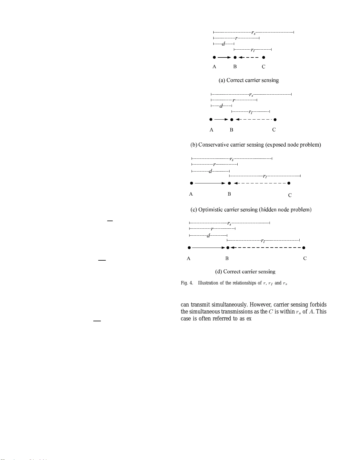
1 Understanding the P aradoxical Ef fects of Po wer Control on the Capacity of W ireless Netw orks Y ue W a ng ∗ John C.S. Lui ∗ Dah-Ming Chiu + ∗ Department of Co mputer Science & Engineering + Department of Information Engineering The Chines e Uni versity of Hong K ong Email: { ywang ,cslui } @cse.cuh k.edu.hk , dmchiu@ie.c uhk.edu.hk Abstract — Recent w orks sho w conflicting results: network ca- pacity may increa se or decre ase with higher transmission po wer under dif ferent scenarios. In thi s work, we want to un derstand this paradox. Specifically , we addr ess the f ollowing questions: (1)Theoretically , should we increa se or decrease tra nsmission power to ma ximize network ca pacity? (2) Theoretically , how much network capac ity gain can we achiev e by power contro l? (3) Under realistic situations, how do po wer control, link schedu ling and routing interact wi th each other? Under whi ch scenarios can we expect a large capacity gain by using higher transmis- sion p ower? T o answer these questions, fi rstly , we prov e th at the optimal n etwork capacity is a non-decreasing function of transmission power . Secondly , we p ro ve that the optimal network capacity can be increased un limitedly by higher t ransmission power in some network confi gurations. Howe ver , when nodes are distribut ed uni fo rmly , th e gain of optimal network capacity by higher transmission power is upper-bounded by a p ositiv e constant. Thirdly , we discuss why network capacity in practice may increase or decrease wi th h igher transmission power under different scenarios usin g carrier sensing and the minimum hop- count routing. Extensive simul ations are carried out to verify ou r analysis. K e ywor ds: Network Capacity , Po wer Contro l, Routing, Link Scheduling I . Introduction W ireless networks have be en activ ely developed for provid - ing ubiq uitous network access in the past d ecades. Recently , wireless mesh networks (WMNs) are co nsidered as a key solution to extend the coverage of the I nternet, espe cially in areas where wir ed networks are expe nsiv e to deploy , e.g., in rural area s. There fore, im proving n etwork capacity is on e of the m ost importan t issues in the research of wire less networks. Roughly speak ing, n etwork capacity is the total end-to- end throug hputs, which we will c arefully define in Section II. V arious techniqu es rang ing fr om p hysical layer to network layer have bee n proposed f or this pu rpose, such as MIMO [1], multi-chan nel multi-rad io [2], high- throug hput routin g [25]– [28], etc. One way to increase network capacity is by lev eragin g transmission power . Th is is effecti ve especially in WMNs wh ere stationar y mesh ro uters usually have sufficient power su pply , for example, th ey can shar e power su pply with street-lamps as cited in [3 ]. In this paper, we study the im pact of power contr ol on the capacity of wireless network s. In par ticular , w e consider wire- less networks where nodes are stationar y and are connec ted in ad-hoc man ner . Under this network setting, power control c an significantly affect network capacity via the inter actions with the link schedu ling and the routing algorith ms. First, many link sch eduling algorithm s in wir eless networks nowadays im plement ca rrier sensing to av oid transmission collisions due to interfere nces 1 . That is, transmitters sense channel states b efore tran smissions and they can transmit only wh en th e sensed no ise strength is below carrier sensing threshold. Power contro l has a tight relatio n with ca rrier sensing. When transmission p ower incr eases, the sensed n oise strength, mainly due to in terference, is more likely beyon d carrier sen sing thresho ld, which ma y redu ce spatial reuse, i.e., the n umber of simultane ous transmissions. Since n etwork capacity dec reases with lower spatial reu se, hig her transmis- sion p ower m ay d ecrease network capacity . Second , power control has a tight relation with ro uting. On th e one hand , higher transmission power m ay redu ce the number of hop s o r transmissions that a sour ce ne eds to r each its destination for a longer transmission ra nge. Since network capacity incre ases with fewer numb er of tran smissions for an app lication-layer packet, highe r transmission power may in crease n etwork ca- pacity . On the o ther hand, bec ause longe r transmission rang e reduces spatial reu se (see Section II), higher transmission power ca n decr ease network capac ity . Consider ing perfect link sched uling, authors in [4] argued that network ca pacity decreases with high er transmission power under the minim um hop-co unt routing . However , som e recent works showed that network capacity actually increases with hig her transm ission power in some scenar ios [ 5] [6]. In this pap er , we system atically ch aracterize the impact of p ower con trol on network capac ity and provide a d eep understan ding on the interesting pa radox : why n etwork capac- ity may increase or decrease with hig her transmission power in different scen arios? Specifically , we address the fo llowing questions: 1) Th eoretically , should we increase or decrease transmis- sion power to max imize network cap acity? 2) Th eoretically , how much n etwork capa city gain can we achieve b y power con trol? 3) Und er realistic situations, h ow d o power co ntrol, link scheduling and r outing interact with each other? Unde r which scenarios can we expect a large capacity gain 1 W e do not consider CDMA at the moment, which applies some other techni ques for interfe rence cance llation. 2 using higher transmission power? The contributions o f this work are as follows: • W e pr ove that the optimal n etwork capacity is a non- decr easing functio n o f transmission power when the network is using the o ptimal link schedulin g an d rou ting. • W e prove that u nder some specific configu rations, the optimal network capacity ca n be increased unlimitedly by h igher tran smission power . Howe ver , when nodes are distributed uniformly over a space, the gain of the optimal network capacity by hig her transmission power is u pper- bound ed by some positiv e con stant. T o the be st of our knowledge, we are the first to prove this pro perty . • W e provide a qu alitati ve an alysis o n the inter actions o f power co ntrol, car rier sensing and the minimum hop- count routing . The later two a re the key featu res co m- monly used in the link sched uling an d routing algorithm s nowadays. Throug h this analysis, we can explain the parado xical effects of p ower contr ol o n in creasing net- work cap acity . T he essential r eason is that carrier sensing and the min imum h op-cou nt rou ting are n ot optimal. W e also provide a taxo nomy of different scenarios wh ere network capacity (may) increase or de crease with h igher transmission power . • Besides the theoretical con tributions, ou r work o ffers some importan t implicatio ns to n etwork desig ners. First, one can redesign th e link scheduling and routing algo- rithms so as to increase network capacity u nder high transmission p ower . Second, we o bserve from simulation that high tr ansmission p ower can significan tly incr ease network cap acity in the networks who se d iameters are within a few h ops, which can find app lications in small WMNs. The rest of th e paper is organ ized as follows. In Section II, we p resent a m odel o f wireless networks and de fine perf or- mance measures. In Section III, we prove the theo retical n et- work capacity gain of power control. In Section IV, we discuss why n etwork capacity in pra ctice may increase o r dec rease with h igher transmission power , co nsidering the interactio ns of power co ntrol, carrier sen sing and the minimum h op-cou nt routing . In Section V, we study h ow ne twork capacity varies with tran smission p ower in different scenarios v ia simulation . In Section VI, we present related works. In Section VII we conclud e our paper . I I . System Model In this section, we first pre sent a phy sical m odel commo nly used in the r esearch of wireless networks [7]. Then we defin e perfor mance measures and some no tations used thr ougho ut this paper . In this paper, we con sider a sta tic n etwork of n nodes which are located on a 2D plane. Nodes are con nected in ad-hoc manner . W e use ( A, B ) to den ote a link transmitting from node A to no de B , an d use | A − B | to d enote th e Euclidean distance between A and B . W e m ake the following assumptions fo r the wireless physical m odel: 1) Common transmission power . All n odes use the same tran smission power . This assumption simp lifies our discussions. Actu ally , the au thors o f the COMPO W ( COMmon POW er) p rotocol showed that per-node (or per-link) p ower contro l can o nly improve network capacity marginally than common power control [4] . 2 ) Sing le ideal chann el. All nodes tra nsmit on an id eal c hannel withou t chan nel fading. Th is assumption simplifies our analysis so that we can focus on under standing this parado x. In pr actice, there are some ph ysical tech nologies such as M IMO whic h can gr eatly mitigate channel fading by using smart a ntennas [1]. 3 ) S ingle transmission rate. All nodes transm it at the same date rate o f W bp s. 4) Corr ect packet r eception ba sed on signa l-to-no ise (SNR) threshold. Let P t be th e transmission power . For a link e , the r eceiv ed signal strength P r at e ’ s r eceiv er is P r = c p P t d α , (1) where c p is a con stant determ ined b y some phy sical p arame- ters, e.g. antenna height, α is the path loss exponen t, varying from 2 to 6 d ependin g o n the environment [9], and d is th e distance fro m e ’ s tran smitter to its receiver (we call it th e length of link e ). W e assum e all c p ’ s are equa l. Thus, by letting P t denote c p P t , we can simplify Eq. (1) as P r = P t d α . (2) For link e , its sign al-to-no ise (SNR) is d efined at its receiv er side, which is S N R = P r P i 6 = e I i + N 0 , (3) where P r is the signal streng th at e ’ s r eceiv er, I i is the interferen ce strength from some o ther transmitting link i to e , an d N 0 is th e white noise. I i is also calculated b y Eq.( 2) except that d here is the distance fr om i ’ s transmitter to e ’ s receiver . The accum ulativ e interfer ence stren gth and N 0 are treated as n oise by e ’ s r eceiv er . No te that N 0 is u sually small comparin g with interfere nce streng th so that we can ignore it. T o suc cessfully r eceiv e a p acket, the f ollowing two co ndi- tions should both be satisfied: P r ≥ H r , ( 4) and S N R ≥ β , (5) where H r is the receiving power thr eshold a nd β is the SNR threshold for decod ing packets correctly . From the ab ove eq uations, on e can der iv e r , the maximu m distance between a tra nsmitter and a receiv er fo r successful packet receptions (the maximum is achiev ed when interferenc e is zero), r = min (  P t N 0 β  1 /α ,  P t H r  1 /α ) . (6) W e refer to r as transmission range . T wo no des can form a link when they are within a distance of r . The in terfer ence range r I of a link e is defined as th e minimum distance between an interferin g transmitter and e ’ s receiver so that e ’ s transmissions are not co rrupted . Let d be 3 the length of e . Fro m Eq. (2)-(3), and igno ring N 0 , we have P t /d α P t /r α I = β , which yields r I = β 1 /α · d (7) W e observe that r I is a constant times of d an d is inde- penden t o f transmission p ower . Another observation is that the silence area for successfu l transmissions of a lin k is propo rtional to the link length. This sug gests that spatial reuse, i.e. the number of simultaneo us transmissions, will decr ease with the lengths of links. Next, we define ne twork capac ity according to [8] 2 , which is fr om the perspective of end-users. W e consider a network G and a set o f flows F . Each flow is associated with a r ate. The rate o f a flow is th e average end-to -end throug hput of th e flow . W e use a vector to deno te th e rates of all flows, n amed flow rate vector . Capa city r egion defines all flow rate vectors that can be suppo rted b y the network. W e define traffic pattern as th e ratio of the rates o f all flows, which can be represented in the vecto r f orm: ( v 1 , v 2 , ..., v | F | ) , where v 2 1 + v 2 2 + ... + v 2 | F | = 1 . Given the traffic pattern, we can obtain a c orrespon ding flow rate vector a · ( v 1 , v 2 , ..., v | F | ) by a scaling factor a . T he network cap acity und er th e traffic pattern of ( v 1 , v 2 , ..., v | F | ) is define d as max a> 0    a · X i =1 ... | F | v i    , (8) , which is the max imum total rates of flows suppo rted by the network. W e illustrate th e above d efinitions by an example. Th ere are f our no des ( A , B , C and D ) and two flows ( f 1 from A to C and f 2 from B to D ) in the n etwork of Fig. 1. So there are thre e links ( ( A, C ) , ( B , C ) and ( C, D ) ) con tending the chann el. Let λ 1 and λ 2 be th e rates o f the two flows, respectively . W e can ea sily calcu late the capacity region of ( λ 1 , λ 2 ) b y the constraint λ 1 + 2 λ 2 ≤ W . Suppose the traffic pattern is ( 1 √ 2 , 1 √ 2 ) , then th e network capacity is 2 3 W when λ 1 = λ 2 = 1 3 W .         Fig. 1. Illustration of the definition of netw ork capacity Equiv alently , we can calculate n etwork capacity as follows. Giv en the traffic patter n ( v 1 , v 2 , ..., v | F | ) , we generate the correspo nding traffic workload vector b · ( v 1 , v 2 , ..., v | F | ) by a large scaling factor b ( b · v i is the traffic workload a ssigned 2 W e adopt thi s definitio n of netw ork capacit y because it isola tes the capa city definiti on from fai rness concerns to the i th flow). Sup pose th at the n etwork d eli vers all traffic workloads in time T , th en the network capacity is b · P i =1 ... | F | v i T . (9) Finally , we define th e network capacity gain of p ower control. Given the wireless network an d the traffic pattern, let C P ( R, S ) be the network capacity when P t = P unde r the routing a lgorithm R and th e link sched uling algo rithm S . R defines the ro utes of each flow , and S d efines wh ether a link can transmit at any time t . W e use C ∗ P ( R ∗ , S ∗ ) or C ∗ P to denote the o ptimal network capacity when P t = P unde r the optimal routing algorith m R ∗ and the optimal link schedu ling algorithm S ∗ . Let P and K P ( K > 1 ) be the minimal and the m aximal transmission power , respectiv ely . Note that P shou ld guaran tee network connectivity ; Otherwise, netw ork capacity is meaning- less since some flows may not be ab le to find routes to rea ch their destinatio ns. W e de fine network capacity gain of power contr ol ( G K ( R, S ) ) by u sing th e routing algo rithm R and the link scheduling algorith m S as G K ( R, S ) = C K P ( R, S ) C P ( R, S ) . (10) Furthermo re, we define the theoretical network capa city ga in of power contr ol ( G ∗ K ), i.e., G ∗ K = C ∗ K P C ∗ P . (11 ) Unless we state other wise, we will use K to denote the ratio of the m aximal transmission power to the minimal transmission power in this pa per . I I I . Theoretical network capac ity g ain o f power control In this section, we der i ve the theo retical capa city gain of power contro l based on the inf ormation- theoretic persp ectiv e. In order to deri ve the optimal network capacity , we ass ume that nodes transmit in a sy nchron ous time-slotted mode and each transmission occupies o ne tim e slot. Fro m n ow on we w ill u se the ph rase ”with high p r o bability” abbreviated as ”whp” to stand f or ”with pr obability appr oaching 1 as n → ∞ ” where n is the nu mber of nodes in the network. The f ollowing theorem states the relation ship between the optimal network capacity and transmission power . Theorem 1: G iven the network top ology a nd the traffic pat- tern, the op timal ne twork c apacity is a n on-decreasing fu nc- tion of the common transmission power . Ther efore , G ∗ K ≥ 1 . Proof: L et S ∗ P ( t ) d enote the set of transmitting lin ks at time slot t whe n P t = P . For any lin k e ∈ S ∗ P ( t ) , its SNR satisfies P r P i ∈ S P ( t ) ,i 6 = e I i + N 0 ≥ β , (12) where P r is the signal strength of e an d I i is the inter ference strength f rom some other transmitting link i to e . Now we set P t = K P ( K > 1 ) and use the same routes an d the same link 4 scheduling sequenc e a s P t = P . W e can see that at time slot t , e ’ s SNR is K P r P i ∈ S ∗ P ( t ) ,i 6 = e K I i + N 0 > P r P i ∈ S P ( t ) ,i 6 = e I i + N 0 ≥ β , (1 3) where we use th e fact that P r and I i are prop ortional to P t . So S ∗ P ( t ) can be sch eduled at t wh en P t = K P for any t . Since R ∗ and S ∗ are o ptimal routin g an d link sched uling, w e have C ∗ K P ≥ C ∗ P by optimality . Remarks: The theorem seems cou nter in tuitiv e but is ea sy to understan d. Basically , given a set of simu ltaneous link s, SNR does n ot dec rease with higher tr ansmission p ower beca use both signal streng th and interferen ce strength incre ase at the same ratio . N etwork capacity can be fu rther imp roved if we can find better rou tes under higher transmission power . Th erefore, theor etically , it is desirab le to u se h igher transmission power to in crease network cap acity . An in teresting qu estion is how mu ch network capa city g ain we can ach iev e by using higher tran smission power . T o answer this que stion, let u s analyze it b ased on the infor mation- theoretic perspective [7]. W ithout loss of gene rality , we scale space and suppo se that n nodes are located in a disc of un it area. Theorem 2: I n general, G ∗ K can be unboun ded whe n n → ∞ . Proof: W e prove it by con structing a sp ecific network. There are 2 m +1 vertical links each with a length of d . The horizontal distance b etween a ny two adjacent vertical lin ks is 2 d . Fig. 2 illustrates five vertical link s where ( A 1 , A 2 ) is th e mid dle link o f the network. A 3 ev enly separates the line between A 1 and A 2 . Also, there are two nod es evenly separ ating the line between any two horizon tally n eighbo ring no des. So there ar e totally n = 12 m + 3 nod es in the n etwork. There is a flow along each vertical link from the to p node to the bo ttom n ode. Let α = 4 and β = 10 in th e physical model. The m aximal transmission p ower K P is set large enough that the transmission range r is mu ch larger th an d and N 0 can be n eglected. Thus, the 2 m + 1 vertical link s can transmit simultaneou sly for any m . T o see this, we can check the SNR of the m iddle link ( A 1 , A 2 ) which suffers the most interferen ce, i.e., S N R ( A 1 ,A 2 ) ≥ K P d 4 2 · P m i =1 K P ( √ d 2 +(2 id ) 2 ) 4 . (14) S N R ( A 1 ,A 2 ) ≈ 11 > β when m → ∞ . Therefore, C ∗ K P is (2 m + 1 ) W or ( 1 6 n + 1 2 ) W . The minimal tr ansmission power P is set so that d > r > 2 3 d . T hus all flows have to g o thr ough A 1 , A 3 and A 2 to rea ch their destinations. For example, the route fr om E 1 to E 2 is thro ugh C 1 , A 1 , A 3 A 2 and C 2 . So C ∗ P is at m ost 1 2 W since ( A 1 , A 3 ) an d ( A 3 , A 2 ) ar e th e bo ttleneck links fo r all flows. Therefo re, G ∗ K is at least ( 1 3 n + 1) , which is unbou nded when n → ∞ . Remarks: The above theorem shows that network capacity can be in creased unlimitedly by using highe r transmission power in some network configur ations. . . . . . . d 2d A 1 A 2 B 1 B 2 C 1 C 2 D 1 D 2 E 1 E 2 A 3 Fig. 2. A network havi ng unbounded G ∗ K Howe ver , n odes p lacement is ap proxim ately ra ndom in many r eal networks. W e will show that G ∗ K is upp er-bounded by a constant whp for netw ork s with uniform node distribution. Before we finally prove this result, we hav e the following lemmas. W e first cite a lemma which was proved in [7] . Lemma 1: F or any two s imultane ous l inks ( A, B ) an d ( C, D ) , we ha ve | B − D | ≥ ∆ 2 ( | A − B | + | C − D | ) , wher e ∆ = β 1 /α − 1 . Remarks: From this lemma, if we draw a disc fo r each link where the center of the disc is the link ’ s receiver and the radius is ∆ 2 times the lin k length, all such d iscs are disjoin t. Note tha t ∆ > 0 because we usu ally have β > 1 in pr actice. Lemma 2: Consider a set of simultan eously tr ansmitting links wher e the length o f any link is at least d . Given a r e gion whose dia meter is 2 R , the numb er of links intersecting the r e gion is upp er-bounded by 1 ∆ 4 (4(∆ + 1) R d + ∆ + 2 ) 2 , where ∆ = β 1 /α − 1 . Proof: See Append ix A-1 . W e define r c as the critical transmission rang e for ne twork connectivity whp . Fro m [ 7], we k now that r c = q log n + k n π n for n nodes u niformly located in a disc o f unit area, wher e k n → ∞ as n → ∞ . Lemma 3: Assume transmission power is sufficiently lar ge so that r > 4 r c . F or a network with uniform n ode distribution, ther e exist s a r oute between a ny two nod es A and B which satisfies the following con ditions whp: (a) fo r a ny relay link on the r ou te, its length is smaller than or equal to 4 r c ; (b) the vertical distanc e fr om any relay no de to the straight-line se gment o f ( A, B ) is at most r c ; (c) the numb er o f h ops between any two r elay no des a 1 and a 2 is not mor e than | a 1 − a 2 | 2 r c + 1 . Proof: See Append ix A-2 . Remarks: Intuitively , the lemm a sh ows that th ere exists a route which can ” approx imate” the straight-line se gmen t of any two n odes whp for a network with unifor m n ode distribution. Theorem 3: A ssume α > 2 and transmission p ower is su f- ficiently la r ge so that r > 4 r c . F or a network with unifo rm node d istrib ution , G ∗ K is b ound ed by a con stant c whp, where c is not depen ding on K or traffic pa ttern . Proof: Let P and K P ( K > 1 ) be the minimal an d max imal transmission power, respectively . Le t S ∗ K P ( t ) b e the set of 5 simultaneou sly transmitting links at tim e slot t wh en P t = K P . T o p rove th is the orem, it is sufficient to prove that f or any t we can sch edule the traffic in S ∗ K P ( t ) in a t most c time slots when P t = P . By optimality , we have G ∗ K ≤ c . W e will construct such c . T o av oid co nfusion here, w e use ”link ” to denote a link when P t = K P and use ”sublink” to denote a lin k when P t = P . Note that we constru ct all sub links fr om their correspo nding links in this pr oof accord ing to Lemma 3. That is, supp ose P is sufficiently large so th at r > 4 r c , we can find the r ela y sub links wh ich satisfy the conditions of Lemm a 3 for each link in S ∗ K P ( t ) whp when P t = P . First, w e will show that such a sublin k is interfered b y at most c 0 sublinks, wher e c 0 is a constan t not dependin g on K or tra ffic patter n. Note that we on ly consider the link s in S ∗ K P ( t ) with a leng th larger than o r equal to r c here, since we can schedu le the links in S ∗ K P ( t ) with a length smaller th an r c using another time slot. W e consider some relay su blink ( A, B ) . I n the prepara tory step, we co unt the nu mber o f sublin ks inter secting the ann ulus U ( i ) of all poin ts lyin g within a distance between ir c and ( i + 1) r c from B , wh ere i ≥ m ( m is a co nstant which we will d etermine later). W e e venly divide U ( i ) in to ⌈ 2 π ( i + 1) ⌉ sectors, each of wh ich has a central a ngle of at most 1 i +1 . Consider such a sector S . It is easy to see that its diameter is not m ore th an 2 r c . So we can draw a disc of ra dius 2 r c , named S ′ , to cover S . Fro m Lemma 3, a r elay sublink deviates from its corr esponding link by a distance of not more than r c . Therefo re, if a sub link intersects S ′ , the shor test distance between its corresp onding lin k a nd S ′ is at least r c . Fig. 3 illustrates the worst case fo r a link (de noted by the d irectional dashed line) whose sublinks intersect S ′ , where the link should at least intersect a d isc of radius 3 r c . Since we consider th e links with a len gth not less than r c , fr om Lemma 2, the number of lin ks whose sublinks intersect S ′ is upp er-bounded by 1 ∆ 4 (4(∆ + 1) 3 r c r c + ∆ + 2 ) 2 = 1 ∆ 4 (13∆ + 14 ) 2 . A sublink cannot intersect S ′ if the sho rtest distance be - tween its transmitter (or rece i ver) and S ′ is larger than 4 r c , since its length is not more th an 4 r c accordin g to Lem ma 3. Therefo re, fo r any link, the nu mber of its corr espond ing sublinks in tersecting S ′ is u pper-bound ed by 2(2+4) r c 2 r c + 1 = 7 .                         ! " # $ % & ' ( ) * + , - . / 0 1 2 3 4 5 6 7 8 9 : ; Fig. 3. Illustra tion of the worst case for a link whose sublinks can intersect S ′ From the a bove re sults, the n umber of sublin ks inter secting the annu lus U ( i ) is upper-bound ed by ⌈ 2 π ( i + 1) ⌉ · 1 ∆ 4 (13∆ + 14) 2 · 7 < c 1 ( i + 2) , wh ere c 1 = 14 π ∆ 4 (13∆ + 14) 2 . Besides, f or a su blink inter secting U ( i ) , the distance f rom its tran smitter to B is not less than ( i − 4) r c . As a result, the to tal interfe rence to B co ntributed by th e sublinks intersecting U ( i ) is uppe r- bound ed by c 1 ( i + 2) · P (( i − 4) r c ) α . Consider th e d isc C ( B , mr c ) of all poin ts lying within a distance mr c from B . Suppose that n o simultaneous trans- missions of the sub links intersecting C ( B , mr c ) are allowed, the SNR of ( A, B ) is lower -boun ded by P (4 r c ) α P ∞ i = m c 1 ( i + 2 ) · P (( i − 4) r c ) α + N 0 = P (4 r c ) α N 0 ( 6 α − 1 m 1 − α + 1 α − 2 m 2 − α ) · c 1 P r α c N 0 + 1 . (15) W e see th at the denom inator of th e last term above app roaches 1 when m → ∞ fo r α > 2 ( In pr actice, we usually have α > 2 [9]. And α = 2 corre sponds to th e free-space path loss model). Sup pose P is sufficiently large so that r > 4 r c , the n we have P (4 r c ) α N 0 > β . So ther e m ust exist some c onstant m making Eq . ( 15) larger th an o r equal to β . Clearly , m o nly depend s on c 1 . Theref ore, ( A, B ) is only interfered by th e sublinks intersecting C ( B , mr c ) . So the num ber o f sublinks interfering ( A, B ) is upp er-bounded by c 0 = 1 ∆ 4 (4(∆ + 1 ) ( m + 1) r c r c + ∆ + 2) 2 · ( 2( m + 4) r c 2 r c + 1) = m + 5 ∆ 4 ((4 m + 5 )∆ + 4 m + 6) 2 , (16) following the similar argume nts above. No te that c 0 is not depend ing on K or traffic patter n. Second, we can co nsider e ach sub link as a vertex . I f a sublink is n ot inter fered by some other su blink, they are assigned b y different colors . Fr om the well-known result of vertex coloring in gr aph th eory , we kn ow that each sublink can be schedu led at least onc e in every c 0 + 1 slots to finish the traffic of S ∗ K P ( t ) . Finally , consider the links in S ∗ K P ( t ) with its length sm aller than r c , we have c = c 0 + 2 , where c is no t d ependin g on K or traffic pattern . Remarks: First, the assum ption of ” the tran smission power is sufficiently large” is n ecessary for G ∗ K to be upper-boun ded. W e illustrate it by an example. Consider th ere is o ne flow transmitting from A to B in a lin ear topolog y . Suppo se there is a direct co mmunica tion b etween A a nd B when P t = K P . So C ∗ K P = W . Suppose the re are m ho ps from A to B and each hop distance is exactly r wh en P t = P , wh ere r is the tra nsmission rang e a nd r = ( P N 0 β ) 1 /α (theoretically , we can assume H r is arbitrarily sma ll). Obvio usly , on ly one hop can transmit su ccessfully at a time to satisfy the SNR requirem ent. So C ∗ P = W m . There fore G ∗ K = m which is unb ound ed wh en m → ∞ . Sec ond, the assumptio n of ”unifor m no de distribution” is n ot n ecessary fo r G ∗ K to be upper-boun ded. Actually , we c an derive th e same result in Theorem 3 if Lem ma 3 hold s for some other rando m n ode distribution, or mo re g enerally , if the route between any two nodes can ”appr oximate” the straigh t line segment of them. 6 In summar y , the optimal network capacity is a non - decr easing fun ction of transmission power . Under some spe- cific configura tions, the optimal network capacity can be increased unlimitedly by high er tran smission p ower . However , when nodes are distributed unifo rmly over a space, the gain of optimal ne twork capacity by higher transmission power is upper-boun ded by som e positi ve constant whp . I V . Pra ctical Network Capacity Ga in of Power Control In th e p revious sectio n we see that network capacity is maximized un der the settings o f ma ximal transmission p ower , optimal ro uting and link scheduling . Howev er, the latter two are NP-hard prob lems [10] [1 1]. In this sectio n, we examine G K by using ca rrier sen sing and the min imum h op-co unt routing , which ar e the key f eatures com monly u sed in the link scheduling and rou ting alg orithms now adays. First, we discuss carr ier sen sing. T o avoid co llisions du ring transmissions, m any c urrent solutio ns requir e transmitters to sense c hannel b efore transmissions. A tran smitter can transmit only when P s ≤ H s , (17) where P s is the noise streng th sensed a t transmitter side and H s is carrier sensing thr eshold . Assume the network is symmetric , that is, P s at transmitter side is equal to P I i + N 0 at r eceiv er side ( Note th at th e a ssumption is of ten inv alid in pr actice). By setting H s = P r β , on e can guar antee th at S N R ≥ β [12] . Howe ver , it is difficult in practice for a transmitter to k now its P r at receiver sid e. T o circu mvent this problem , we c an con servati vely estimate P r by H r . So we have H s = H r β . (18) H s in curren t settings is mo re o r less this value, e. g. Lucen t ORiNOCO wireless card [1 3]. For better illustrations, we introdu ce carrier sensing range r s , wh ich is de fined as the m aximum distance that th e trans- mitter can sense th e transmissions of an inter fering transmitter . From Eq. (2) by letting P r = H s , we have r s =  P t H s  1 /α . (19) Suppose H r ≥ β N 0 , which is usually th e case in p ractice [14]. From Eq. (6), (1 8) a nd (19), we have r s = β 1 /α · r. (20) Comparing with Eq. (7), we see that r s is equal to th e interferen ce range of the maximum link length. Fig. 4 illustrates the relatio nships of r , r I and r s by a network of a tra nsmitter A , a receiver B and a interfer ing transmitter C . Her e, we use d to de note | A − B | . Th e network is not symme tric as A is fur ther from C tha n B is. In Fig. 4(a), C causes packet co llisions of ( A, B ) as it is within r I of B . Howe ver , C is also within r s of A . So A will not tr ansmit and thus av oid collisions wh en it senses the tran smissions of C . I n Fig. 4 (b), C is moved ou tside r I of B and thus becomes a non -interfer ing transm itter to ( A, B ) . So A an d C < = > ? @ A B C D E F GH I J K L M NO P Q R S T U V W X Y Z[ \ ] ^ _ ` a bc d e f g h i j klm n o p q r s t u v wx y z { | } ~                                 ¡ ¢ £ ¤ ¥ ¦ § ¨ ©ª« ¬  ® ¯ ° ± ² ³ ´ µ¶ · ¸ ¹ º » ¼ ½ ¾ ¿ À ÁÂ Ã Ä Å Æ Ç È É Ê Ë Ì ÍÎÏ Ð Ñ Ò Ó ÔÕÖ × Ø Ù Ú Û Ü Ý Þ ß à á â ã ä å æ ç è é ê ë ì í î Fig. 4. Illustration of the relationshi ps of r , r I and r s can tra nsmit simultaneously . Howev er, carrier sensing forbids the simultaneous transmissions as the C is within r s of A . This case is often refer red to as exposed terminal (n ode) pr o blem . Fig. 4 (c) and (d) illustrate the scen arios when we increase d . By Eq. (7), r I also incre ases a nd it is n ot fully covered by r s here. In Fig . 4(c), there will be a lot of collisions for ( A, B ) as C is in side r I of B and outside r s of A . T his case is often referr ed to as h idden terminal (nod e) pr o blem . Currently , some MAC protocols (e.g. 8 02.11 ) use the b ackoff mechanism to redu ce co llisions in this case. In Fig . 4(d), C is moved outside r I of B an d becomes a non-in terfering transmitter to ( A, B ) . So A and C can transmit simultaneou sly . Exposed terminal pro blem is liable to occ ur when the length of a link is small, while hidden term inal pro blem is liab le to occur when the length of a lin k is large. Th e rad ical reason is that car rier sensing uses fixed H s and op erates at transmitter side, which can no t estimate interferen ce accurately . Therefo re, e ven under th e optimal ro uting, network capa city can d egrade with h igher transmission power by u sing car rier 7 sensing. For example, consider a network with all one-ho p flows, higher transmission power increa ses r s , which can reduce spatial reuse and thus d ecrease network capacity . Howe ver , the cur rent H s may not be too con servati ve under the minimum hop-c ount rou ting, beca use this kind of routing prefers the link s of lon gest lengths (appro aching r ), wh ich is close to the case wh en we der i ve Eq. (18). Consider a link with a leng th d , the range that r s cannot cover r I is d + r I − r s = d + β 1 /α d − β 1 /α r , (21) which is appr oximately r when d ≈ r . This implies that ther e can be more hidden terminals when r becomes larger un der the minimu m ho p-cou nt ro uting. Next, we discu ss the minimum h op-co unt routin g. The authors of [4] argu ed that even u nder optimal link schedu ling network ca pacity by using the minimu m hop-c ount r outin g is propo rtional to 1 r . (22) So G K = ( 1 K ) 1 /α by Eq. (6). Their in terpretation is as follows. The network capacity consump tion o f a flow is pr oportio nal to the nu mber of hops the flow trav erses, i.e. 1 r . Spatial reuse is pro portion al to 1 r 2 . Network cap acity is p ropor tional to spatial reuse and inver sely proportio nal to the network capacity consump tion per flow , i.e. 1 r . W e make some comm ents on Eq. (22). First, althoug h it pro perly char acterizes the order o f network capacity as a fun ction of r , it h as som e deviations fro m practice. For example, the network diameter (in ter m of the nu mber of hops) m ay be so small that th e spatial reuse m ay n ot decre ase as m uch as 1 r 2 due to edg e effect 3 . As a result, the network capacity may increase with larger r . Fig. 5 shows an examp le where there are five nodes and two flows of equal rate in the network. When the transmission power is low , both flows need to trav erse th e centered no de to r each their respective destinations. Since the re are fo ur links conten ding the chann el, the network ca pacity is 1 4 W · 2 = 1 2 W . When we incr ease the transmission p ower so that packets can be transmitted d irectly from sources to destinations, there are two links contending the channel, and ne twork capacity is 1 2 W · 2 = W . Actually , the spatial re use here is always one transmittin g link p er time slot for any p ower le vel due to edge effect. The network capacity increases with high er transmission p ower due to a le ss n umber of hops per flo w . Second, it may not hold for the networks with non-u niform link load distribution . Fig.6 shows an example where there are k flows of eq ual r ate trav ersing throug h the centered node. T he link load d istribution is non -unifor m here as the centered node is the biggest bottleneck. It is easy to see that the spatial reuse decreases as 1 r 2 here. Howe ver , the network capacity does no t decr ease as 1 r . T o see this, we consider two specific cases. In the first c ase of usin g the minimal transmission power , eac h flow is m -ho p ( m >> 2 ) . So there are at least 2 k links neigh boring the center ed nod e, resulting in the network cap acity o f at m ost W 2 k · k = 1 2 W . 3 In here, the edge effe ct m eans that the network diameter is so small that most links are near the periphery of the netw ork In the second case of using the maximal transmission power , each flo w is 1 -hop. So there are k links contending the channel, resulting in the network capacity of W k · k = W . ï ð ñ ò ó ô õ ö ÷ ø Fig. 5. An example of a network with a small network diameter ù ú û ü ý þ ÿ         . . . Fig. 6. An example of a network with non-uniform load distrib ution Based on the above o bservations, o ne can explain why net- work capacity sometimes increases with h igher transmission power unde r the m inimum hop-co unt rou ting [5] . In summar y , curren t car rier sensing and the minimum hop - count routing d o n ot guarantee G K ≥ 1 and m ay lead to sig- nificant capacity degrada tion with higher transmission power . Howe ver , network capa city may increase significantly with higher tran smission p ower in some scenario s, e.g. in n etworks whose d iameter is with in a sma ll number of hops. Therefor e, there is a paradox on whether to use higher transmission power to increase network capacity in practice. V . Simulat ion Results In this section, we examine the impact of power control on network capacity via simulation . W e use carrier sensing and the minimum hop-co unt rou ting as th e lin k scheduling and routing algorithms in our simulations. Our essential goals are to verify our analysis in th e previous section and to find ou t under which scenarios we can expect a large ne twork cap acity gain b y using high transm ission p ower . W e use the wireless physical m odel described in Section II. W e set α = 4 for simu lating th e two-ray gr ound path loss model [ 9]. W e set β = 10 and H r = − 81 dBm [1 4]. Therefo re, H s = 1 10 H r by Eq. (18). W e ign ore N 0 which is usually much smaller than the interfe rence stren gth. For b etter illustrations, we u se the tran smission range r to re present the transmission p ower . W e increase the transmission power so that r = 25 0 m, 500 m, 750 m an d 1000 m . Actually , o ne can 8 change r p ropor tionally and scale network top ologies at the same time to obta in the sim ilar simulation results. W e implem ented a TDMA simulato r fo r perfor mance eval- uation. That is, nodes transmit in syn chron ous time- slotted mode and e ach DA T A transm ission and its A CK occupies one time slot. Transmitters sense th e chann el one by o ne at the beginnin g of each time slot. A tran smitter will transmit a D A T A packet when P s ≤ H s and its backoff timer expir es. The recei ver returns an A CK to the transmitter when it receives the packet successfully . I f the transmitter doe s not receive an A CK due to packet c ollision, it will carry out the exp onential backoff. The b ackoff mechan ism is similar to that of 802 .11 except that we backoff the time slot h ere. W e ca lculate n etwork capacity accor ding to Eq. (9). W e assign a traffic work load to each flow befo re simu lations start and measure the duration until all flows finish de li vering its traffic worklo ad. In o ur simulations, each flow has a equal traffic workload of 5 00 eq ual-sized p ackets. W e gene rate CBR traffic for each flo w until comp leting its tra ffic workload. The CBR rate is set large eno ugh to satura te the network . Besides, the packet buffer in each node is set sufficiently large since we do not con sider qu eue managem ent at the m oment. There are other factors that affect n etwork capacity in practice such as sophisticated collision resolution mechan isms, TCP congestion contr ol and queue man agement. However , by isolating these factors, we can better u nderstand th e key roles of car rier sensing an d the min imum hop-cou nt routin g on network capacity . For simp licity , in the following experiments, we use CS to denote car rier sen sing an d use HOP to deno te the minimu m hop-co unt routing . W e imple mented a centralized li nk schedul- ing, nam ed Cen , as a benchmar k, which sched ules links one by on e in a centr alized and collision-fr ee way and thus ensure s maximal spatial reuse. In each e xper iment, we take the a verage of all simulation results fo r ten networks. In the first experiment, we study the in teraction of power control and c arrier sensin g by co nsidering one-h op flows so as to isolate the intera ction o f routin g. Experiment 1 Network ca pacity vs Power in a rand om network with one-h op flows . Ther e are n = 2 00 no des unifor mly placed in a squar e of 3000 m × 300 0 m, which form a conn ected n etwork when r = 250 m . Each node ran domly commun icates with one of its nearest neighb ors. Fig. 7 shows the n etwork cap acity as a fu nction of r . Obviously , the n etwork cap acity b y u sing Cen is almost a constant in this scenario . Howe ver , wh en we use CS, higher transmission power causes mo re exposed term inals a nd de- crease n etwork cap acity , since the c arrier sensing th reshold is fixed. In the following experimen ts, we study the interactio n of power control, carrier sensing and the minimum ho p-coun t routing by conside ring multi-h op flo ws. Experiment 2 Network ca pacity vs Power in a rand om network with multi-ho p flows an d small network d iameter (in terms of the n umber of h ops). T here ar e n = 2 0 no des unifor mly placed in a squar e of 1000 m × 100 0 m, which form a conn ected n etwork when r = 250 m . Each node ran domly commun icates with any other nod e in th e network. 250 500 750 1000 0 5 10 15 20 r (m) Network Capacity (#packets/slot) CS Cen Fig. 7. E xperiment 1: Network capaci ty as a function of r Fig. 8(a) shows th e n etwork capacity as a fu nction of r . First, in a sharp con trast to Eq. ( 22), the network capa city by using HOP significantly increases wit h r . The reason is that the network diamete r is so small (4 -6 hop s) that the spatial reuse only decr eases slightly with larger r , as shown in Fig.8(b). Actually , only a f ew link s can transmit simu ltaneously in th is scenario due to edg e effect. HOP m inimizes the number of hops th at flows tr av erse, as shown in Fig.8(c), which is the dominan t factor for the sign ificant in crease of network capac- ity . Seco nd, CS works reasonab ly well in this expe riment, as compare d with Cen (see Fig.8(b) ). The reason is that HO P prefers longest forwardin g links for multi-h op flows, wh ich is close to the case tha t we derive H s in Eq. (18). Experiment 3 Network capacity v s Power in a g rid network with multi-ho p flows and la r ge n etwork dia meter (in terms of the numb er of hop s). There are n = 62 5 nodes plac ed in a 25 × 2 5 grid. There is a d istance o f 200 m between any two h orizonta lly or vertically neigh boring n odes. There are 25 flows fr om the leftm ost no des to th e righ tmost n odes horizon tally and 25 flows from the to pmost nodes to the bottomm ost nod es vertically . This con figuration en sures a large network diam eter an d uniform link load distribution. W e o bserve that the network capacity decreases significantly with larger r , as sh own in Fig. 9, beca use of th e sig nificant decreasing of spatial reuse u nder the minimu m hop -count routing . W e also p lot the network c apacity by using HOP and Cen, which confirms our explan ation. W e also test the rand om n etworks with multi-ho p flows and a lar ge network dia meter . W e observe that the network capacity significantly de creases with larger r in this scenar io whe n n is sufficiently large. In su mmary , the following conclusio ns can be made from our analysis (Section IV) and simulations. When we use carrier sensing and the minimu m ho p-coun t routing , • In th e n etworks with one-ho p flows , the network capacity significantly dec reases with hig her transmission power due to exposed te rminal prob lem. • In the networks with mu lti-hop flows an d a small n etwork diameter of a few hops , the n etwork capacity can incr ease significantly with higher tr ansmission power because th e edge effect makes spatial reu se only decrease slightly with larger r . This c an find applications in small WMNs. Currently , many WMNs tend to have a sm all network diameter (in term of the numb er of h ops), b ecause the 9 250 500 750 1000 0 0.2 0.4 0.6 0.8 1 r (m) Network Capacity (#packets/slot) HOP+CS (a) Network capaci ty as a functio n of r 250 500 750 1000 0 0.5 1 1.5 2 r (m) Spatial reuse (#transmissions/slot) HOP+CS HOP+Cen (b) A vg. spatial reuse as a functi on of r 250 500 750 1000 1 1.5 2 2.5 3 3.5 4 r (m) #Hops per flow HOP+CS (c) A vg. number of hops per flow as a function of r Fig. 8. E xperiment 2 end-to- end thro ughpu t of a flow drop s sign ificantly with an increasing num ber of ho ps [ 7] [15]. • In the n etworks of multi-hop flo ws a nd a lar ge network diameter , there are two s ubc ases. Under uniform li nk lo ad distribution , the network cap acity decreases significantly with highe r tr ansmission power as shown in Eq. (2 2); Under non-u niform link load distribution , it is hard to make a co nclusion. The network capa city may incre ase with highe r tran smission power as illustrated by Fig. 6. V I . Re lated W o rk In this section, we present related work and highlight o ur contributions. Research on power con trol can be classified into two classes: energy or iented an d capacity orien ted. The first class of works focus on en ergy-efficient power control [16] [17] [1 8]. The ap- plication is in mobile ad hoc n etworks ( MANETs) or wireless sensor n etworks (WSNs), where nodes h av e limited b attery life. Low transmission po wer is preferr ed here to maximize the 250 500 750 1000 0 0.5 1 1.5 r (m) Network Capacity (#packets/slot) HOP+CS HOP+Cen Fig. 9. E xperiment 3: Network capaci ty as a function of r throug hput per unit of energy con sumption, while m aximizing overall n etwork capacity is the secondary con sideration. As a result, their solutions often achie ve moderate network capacity . The second class of works f ocus o n capacity- oriented power control. T he application is in WMNs wh ere me sh r outers h av e sufficient power sup ply and max imizing network ca pacity is the first consid eration. Authors in [4] ind icated that network cap acity d ecreases significantly with higher tran smission power under the mini- mum ho p-coun t routing an d they sug gested using the lowest transmission power to maximize n etwork capacity . There are a lot of works f ollowing this suggestion , e.g . [ 19] [20], and they observed capacity improvemen t b y using lower transmission power . Howev er, there is an oppo site argu ment recen tly . Park et al showed via simulation that network capacity so metimes increase with higher transmission power [5]. Behzad et al formu lated the p roblem o f power con trol as an optimiz ation problem an d proved th at network cap acity is ma ximized b y proper ly increasing transmission power [6]. W e also proved that th e optimal network capacity is a non-d ecreasing f unction o f com mon tran smission power in a simpler way . Fur thermore , we ch aracterized the theoretical network capacity ga in of power contr ol. Besides, we stud ied the inter actions o f power co ntrol, carr ier sensing and the minimum hop- count routing. As a result, we explain ed the above paradox successfully f rom bo th th eoretical and practical perspective. Our work pr ovides a deep understand ing on the structur es of th e power control pr oblem and can b e seen as an extension to [4]- [6]. Carrier sensing recently attr acts attention s in th e area of wireless network s. Many resear chers noticed that carrier sens- ing can significantly affect spatial reuse and th e cu rrent car rier sensing thre shold is not optimal in many cases. Xu et al indicated that R TS/CTS is not sufficient to a void c ollisions and larger carr ier sensing rang e ca n h elp to some extend [21]. Y ang et al showed that the M A C layer overhead has a gr eat impact on cho osing car rier sen sing thresho ld [22 ]. Zhai et al considered m ore factors on choosing ca rrier sensing thre shold such as different data rates a nd on e-hop (or mu lti-hop) flows [23]. Th ey showed that network cap acity may suffer a sig- nificant d egradation if any of these factors is not considered proper ly . Kim et al rev ealed that tuning transmission power has the same effect on maximizing spatial reu se as tuning carrier sensing threshold [24] . 10 There are some works on high- throug hput r outing recen tly . ETX uses expected p acket transmission times as the rou ting metric so as to filter p oor ch annel-qu ality links in fadin g chan- nels [ 25]. WCETT extend s ETX for multi-chan nel wireless networks by also considerin g con tention time and channe l div ersity [2 6]. MTM uses packet transmission dur ation as the routing metric in d iscovering h igh-thr oughp ut routes in mu lti- rate wireless networks [27]. ExOR takes a d ifferent appr oach which forwards packets op portun istically in fading channels [28]. V I I . Conclusion This w ork thorou ghly studies the impact of power control on network capacity from both theoretic and practical perspective. In the first part, we pr ovided a fo rmal pr oof that the optim al network ca pacity is a non -decreasing function o f comm on transmission power . Then we ch aracterize the theore tical ca- pacity gain of power control in the case of the op timal network capacity . W e proved that the optima l network c apacity can b e increased unlim itedly with higher tran smission power in some network co nfiguratio ns. Howe ver , the incr ease of network capacity is bound ed by a constant with higher transm ission power whp for th e networks with unifor m node distribution. In the secon d p art, we analy zed why n etwork capacity increases or de creases with higher transmission po wer in dif ferent scenarios, by using carrier sensing and the minimu m ho p- count r outing in practice. W e also cond uct simulation s to study this p roblem und er different scenario s suc h as a small network diameter vs a large network diameter and on e-hop flows vs multi-ho p flows. Th e simu lation r esults verify our analysis. In particular, we o bserve th at network capacity can be significantly impr oved with h igher transmission power in the n etworks with a small n etwork diameter, wh ich can find applications in small WMNs. R E F E R E N C E S [1] D. Gesbert, M. Shafi, D. Shiu, P .J. Smith, and A. Naguib, ”From Theory to Practice : An Ove rvie w of MIMO Space-T ime Coded Wire less Systems, ” IEEE J. Selcte d Areas in Comm. , vol. 21, pp. 281-301, 2003. [2] J. Mo, H.-S. W . So, J. W alrand, ”Comparison of Multi-channe l MAC Protocol s, ” Procs., MSW iM , pp. 209-218, 2005. [3] ”Nortel: W ireless Mesh Ne twork Solution” , http:// www .nortel.com/solu tions/wrlsmesh/ , 2007. [4] S. Narayanaswamy , V . Kawadia, R. S. Sreeni va s, and P . R. Kumar , ”Po wer Control in Ad-hoc Networks: Theory , Archi tecture, Algori thm and Implementa tion of the COMPOW Protocol, ” Procs., Euro pean W ire less Confer ence , 2002. [5] S.-J. Park, R. Si v akumar , ”Load-Sensi ti ve Transmission Power Control in W ireless A d-hoc Networks, ” Procs., GLOBECOM , vol. 1, pp. 42-46, 2002. [6] A. Behzad, I. Rubin, ”High Tra nsmission Powe r Increases the Capacit y of Ad Hoc Wirel ess Networks, ” IEEE T rans. on W irele ss Comm. , vol. 5(1), pp. 156-165, 2006. [7] P . Gupta, and P . R. Kumar , ”The Capacity of W ireless Networks, ” IEEE T rans. on Infomation Theory , vol. 46, no. 2, pp. 388-404, 2000. [8] M. Kodia lam and T .Nandagopa l, ”Chara cterizi ng the capacity region in multi-rad io multi-chann el wireless mesh networks, ” Procs., MOBICOM , pp. 73-87, 2005. [9] David Ts e and Pramod Vi svan ath, ”Fundamenta ls of Wire less Comm u- nicat ion, ” Cambridge Univer sity P re ss , 2005. [10] K. Jain, J. Padhye, V . N. Padmanabha n, and L. Qiu, ”Impact of Interfer- ence on Multi-hop W ireless Networ k P erformanc e, ” Procs., MOBICOM , pp. 66-80, 2003. [11] G. Sharma, R. Mazumdar , and N. Shroff, ”On the Comple xity of Scheduli ng in Wirel ess Netw orks, ” Procs., MOBICOM , pp. 227-23 8, 2006. [12] J. Zhu, X. Guo, L. L. Y ang, W . S. Conner , S. Roy , and M. M. Hazra, ”Adapti ng Physical Carrier Sensing to Maximize Spatia l Reuse in 802.11 Mesh Networ ks, ” W ireless Communicatio ns & Mobile Computing , vol. 4(8), pp. 933-946, 2004. [13] ”Hardwa re Specifica tions of Lucent ORiNOCO W ireless PC Card, ” http:// www .orinocowir eless.com/. [14] ”IEEE 802.11a. Pa rt 11: Wire less LAN Medium Acce ss Control (MAC ) and Physica l Layer (PHY) Specifica tions: High-speed Physica l L ayer in the 5 GHz Band, ” Supplement to IEEE 802.11 Standar d , Sep. 1999. [15] J. Bicket, D. Aguayo, S. Biswas, and Robert Morris, ”Archite cture and Eva luation of an Unplanned 802.11b Mesh Netw ork, ” Procs., MOBICOM , pp. 31-42, 2005. [16] M. B. Pursley , H. B. Russell, and J. S. W ysocarski, ”Energ y-Efficie nt Tra nsmission and Routing Protocols for Wirel ess Multiple-hop Networ ks and Spread Spectrum Radios, ” Procs., EUROCOMM , pp. 1-5, 2000. [17] E.-S. Jung and N. H . V aidya, ”A Power Control MA C Protocol for Ad Hoc Networks, ” P rocs., MOBICOM , pp. 36-47, 2002. [18] J. Gomez, A. T . Campbell, M. Naghshineh , and C. Bisdikian, ”P AR O: Supporting D ynamic Power Controlled Routing in Wirel ess Ad Hoc Networ ks, ” A CM/Kluwer Journal on W ire less Networks , vol. 9(5), pp. 443- 460, 2003. [19] A. Muqattash, M. Krunz, ”Power Controll ed Dual Channel (PCDC) Medium Access Protocol for Wirel ess Ad Hoc Networks, ” Procs. INFO- COM , vol. 1, pp. 470-480, 2003. [20] A. Muqatt ash and M. Krunz, ”A Single-Channe l Solution for Transmis- sion Power Control in W irele ss Ad Hoc N etw orks, ” Procs., MOBIHOC , pp. 210-221, 2004. [21] K. Xu, M. Gerla, and S. Bae, ”How ef fecti ve is the IEEE 802.11 R TS/CTS handshake in ad hoc networks, ” Procs., GLOBECOM , 2002. [22] X. Y ang and N. H . V aidya, ”On the Physical Carrier Sensing in W ireless Ad Hoc Networks, ” Procs., INFOCOM , 2005. [23] H. Z hai and Y . Fang, ”Physical Carrier Sensing and Spatial Reuse in Multira te and Multiho p Wi reless Ad Hoc Networks, ” Procs., INFOCOM , 2006. [24] T .-S. Kim, J. C. Hou, H. Lim, ”Improving Spatial Reuse through Tuning Tra nsmit Power , Carrie r Sense Threshold, and Data Rate in Multihop W ireless Networ ks, ” Procs., MOBICOM , pp. 366-377, 2006. [25] D. S. J. De Couto, D. Aguayo, J . Bicket , and R. Morris, ”A high- throughput pat h m etric for mult i-hop wireless routing, ” Procs., MOBICOM , pp. 134-146, 2003. [26] R. Draves, J. Padhye , and B. Zill, ”Routing in Multi-ra dio, Multi-hop W ireless Mesh Networks, ” Procs., MOBICOM , 2004. [27] B. A werbuch, D. Holmer , and H. Rubens, ”The Medium Time Metric : High Throughput Route Selection in Multi -rate Ad HocW ireless N et- works, ” Mobile Networks and Applicatio ns , vol. 11, pp. 253-266, 2006. [28] S. Biswas, R. Morris, ”ExOR: Opportuni stic Multi-hop Routin g for W ireless Networ ks, ” Procs. SIGCOMM , pp. 133-144, 2005. Ap pendix A-1: The proof of Lemma 2 Proof: W e ca n d raw a disc ( C R ) of radius R to c over the giv en region. W e calcu late th e n umber of simultaneou s links inter secting C R . Let l be the len gth of the longest link. Obviously , we can draw a disc C R + l to cover all links intersecting C R , where the ce nter of C R + l is that o f C R and its radiu s is R + l . By Lem ma 1, each r eceiv er occup ies at least an area o f 1 4 π ∆ 2 d 2 . When l < 2 R + d ∆ , the numbe r of links in C R + l is upper-boun ded by π ( R + (1 + ∆ 2 ) l ) 2 1 4 π ∆ 2 d 2 ≤ 1 ∆ 4 (4(∆ + 1) R d + ∆ + 2) 2 . (23) The u pper bo und of the above equatio n is obtained wh en l = 2 R + d ∆ . When l ≥ 2 R + d ∆ , fro m Eq. ( 7), we can easily see tha t th e silence area ( A l ) of the longest link covers C R , as illustrated in Fig. 10. Because all the o ther simultaneou s transmitters should be outside A l , for any oth er link intersecting C R , its length is at least the sho rtest distance from th e circ le of A l to the circle o f C R , which is (1 + ∆) l − l − 2 R = ∆ l − 2 R in the worst case. By Lemma 1, eac h receiver o ccupies an area of 11 at least 1 4 ∆ 2 π (∆ l − 2 R ) 2 . So the numb er o f link s in C R + l is upper-boun ded by π ( R + (1 + ∆ 2 ) l ) 2 1 4 ∆ 2 π (∆ l − 2 R ) 2 ≤ 1 ∆ 4 (4(∆ + 1) R d + ∆ + 2) 2 . (24) The u pper bo und of the above equatio n is obtained wh en l = 2 R + d ∆ . Com bining the above two cases of l , we proved this lemma.                 Fig. 10. Illustration of C R , C R + l and A l Ap pendix A-2: The proof o f Lemma 3 Proof: W e prove it b y constru cting such a ro ute. If | A − B | ≤ 4 r c , then ( A, B ) itself is th e desired route. Otherwise, we d i vide the straig ht-line segment o f ( A, B ) into small segments of 2 r c until reachin g B . Then we dr aw a small d isc C r c ( i ) of radius r c to cover each small segment, where i = 1 , 2 , ..., ⌈ | A − B | 2 r c ⌉ . Fig. 11 illustrates the case wh en ⌈ | A − B | 2 r c ⌉ = 3 . For better illustration s, we define the x axes with its origin at A and its direction fro m A to B , and d efine the y axes vertical to x . W e can see that the coo rdinate of th e cente r of C r c ( i ) is ((2 i − 1) r c , 0) . T he probab ility of no no de lyin g in C r c ( i ) is (1 − π r 2 c ) n . Since | A − B | is up per-bounded by the diameter of the disk of unit area, i.e. 2 √ π , the pro bability that we can select at least one no de in each C r c ( i ) is lower- bound ed by (1 − (1 − π r 2 c ) n ) 2 √ π · 2 r c , which appro aches 1 as n → ∞ . Since r > 4 r c , we can conn ect the selected nodes to fo rm a ro ute f rom A to B . It is easy to see that th e route satisfies the condition s of this lemma.         ! " # $ % & ' ( ) * + , - . Fig. 11. Dividin g ( A, B ) into s mall segment s of 2 r c