On the Asymptotic Behavior of Selfish Transmitters Sharing a Common Channel

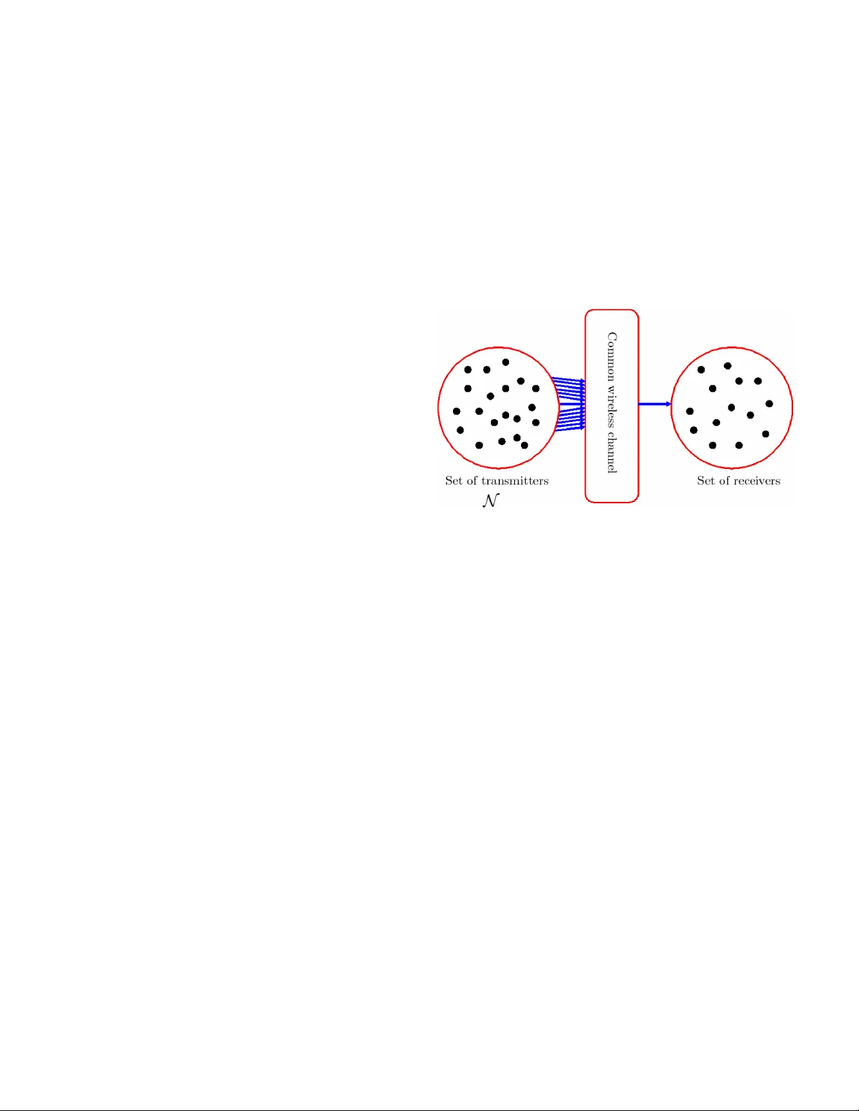
1 On the Asymptotic Beha vior of Selfish T ransmitters Sharing a Common Channel Hazer Inaltekin ∗ , Mung Chiang ∗ , H. V incent Poor ∗ , Stephen B. W icker † , ∗ Department of Electrical Engineering, Princeton Uni versity , Princeton, NJ 08544 Email: { hinaltek, mchiang, poor } @princeton.edu † School of Electrical and Computer Engineering, Cornell Uni versity , Ithaca, 14850 Email: wicker@ece.cornell.edu Abstract — This paper analyzes the asymptotic behavior of a multiple-access network comprising a large number of selfish transmitters competing for access to a common wireless com- munication channel, and having different utility functions for determining their strategies. A necessary and sufficient condition is given for the total number of packet arrivals from selfish transmitters to con verge in distribution. The asymptotic packet arrival distribution at Nash equilibrium is shown to be a mixture of a P oisson distribution and finitely many Bernoulli distributions. I . I N T RO D U C T I O N T o in vestigate the behavior of a multiple-access communica- tion network consisting of large number of selfish transmitters, we consider the network model depicted in Fig. 1. In Fig. 1, each transmitter in the transmitter set has an intended receiv er in the receiv er set. In the context of cellular networks, the transmitter set consists of mobile users requesting uplink reservations to communicate with a base station. In a more general setting, it can be thought of as containing some number of wireless transmitters that are closely located in a wireless ad-hoc network, and that are willing to communicate with another close-by node. The results in this paper can be viewed as characterizing the local behavior of dense wireless networks containing selfish nodes and using a collision channel model at the medium access control (MAC) layer . The collision channel model has been extensi vely used in the past (e.g., [1], [2]), and it is used to characterize the behavior of networks using no power control and containing nodes with single packet detection capabilities. The protocol model defined in [3] is a variation of the collision model. A. Game Definition W e assume that transmitter nodes always hav e packets to transmit, and a transmission fails if there is more than one transmission at the same time. The cost of unsuccessful transmission of node i is c i ∈ (0 , ∞ ) . A likely meaning that can be attributed to c i ’ s is the useless po wer expenditure caused by failed packets. If a transmission is successful, the node that transmitted its packet successfully gets a normalized utility of 1 unit. W e model this situation by using a strategic game G ( n, c ) , which is defined formally as follo ws: This research w as supported in part by the National Science F oundation under Grants ANI-03-38807 and CNS-06-25637. Fig. 1. Network model in which n selfish transmitters contend for the access of a common wireless communication channel to communicate with their intended receivers in the receiv er set. Definition 1: A heter ogenous one-shot random access game with n transmitter nodes is the game G ( n, c ) = hN , ( A i ) i ∈N , ( u i ) i ∈N i such that N = { 1 , 2 , . . . , n } is the set of transmitters, A i = { 0 , 1 } for all i ∈ N , where A i is the set of actions for node i and 1 means transmission and 0 means back-of f, c = ( c i ) i ∈N wher e c i is the cost of unsuccessful transmission for node i , and the utility function u i for all i ∈ N is defined as: u i ( a ) = 0 if a i = 0 , u i ( a ) = 1 if k a k l 1 = 1 and a i = 1 , u i ( a ) = − c i if k a k l 1 ≥ 2 and a i = 1 . In Definition 1, k · k l 1 denotes the l 1 norm for vectors in R n , and is thus the sum of the absolute v alues of the components of a vector . If c i = c > 0 for all i ∈ N , then we will denote G ( n, c ) by G ( n, c ) , and call it a homogenous one-shot random access game. B. A Note on Notation P o ( λ ) and B er n ( p ) will indicate a Poisson distribution with mean λ and a 0-1 Bernoulli distrib ution with mean p , respectiv ely , as well as the generic random v ariables with these distributions. For an y giv en two discrete distributions µ and ν on the set of integers Z , d V ( µ, ν ) denotes the variational distance between them, which is defined as d V ( µ, ν ) = P z ∈ Z | µ ( z ) − ν ( z ) | . If X and Y are random v ariables with distributions µ and ν , we sometimes write d V ( X, Y ) in stead 2 of d V ( µ, ν ) for ease of understanding. If one of the arguments of d V contains a summation of some random variables, this refers to the con volution of their respectiv e distrib utions. If a sequence of probability distributions { µ n } ∞ n =1 con- ver ges (in the usual sense of con ver gence in distribution) to another probability distribution µ , we represent this con ver- gence by µ n ⇒ µ as n → ∞ . As in standard terminology , we call a Nash equilibrium a fully-mixed Nash equilibrium (FMNE) if all of the transmitters transmit with some positi ve probability in (0 , 1) at this equilib- rium. W e call a Nash equilibrium a pure str ategy Nash equilib- rium if all transmitters choose their actions deterministically . Therefore, any given transmitter i ∈ N either transmits or backs-off with probability one at a pure strategy equilibrium. X ( n ) i is the 0-1 random variable showing the action chosen by transmitter i ∈ N when the game G ( n, c ) is played. As noted before, 0 means back-off, and 1 means transmit. Let p i,n denote the transmission probability of transmitter i when there are n transmitters contending for the channel access. Also let S n represent the total number of packet arri vals when there are n transmitters contending for the channel access. Note that S n = P n i =1 X ( n ) i . F or a given set N 0 , |N 0 | will represent the cardinality of this set. C. Nash Equilibria of G ( n, c ) The transmission probability vector at which all nodes back-off with probability one is not a Nash equilibrium of G ( n, c ) since an y node can obtain positive utility by setting its transmission probability to a positive number gi ven the fact that others do not transmit. Therefore, there is an incenti ve for nodes to de viate from the strategy profile at which all of them back-off. As a result, at Nash equilibria of G ( n, c ) , we expect to observe some of the transmitters transmitting with some positive probabilities and the remaining back-off with probability one. T o further inv estigate this point, let π : S ∞ n =2 R n + → R + be such that for any c ∈ S ∞ n =2 R n + , π ( c ) = Q i c i 1+ c i . The following theorem from [4] characterizes the Nash equilibria of this game. Theor em 1: Let X ( n ) i be the action chosen by transmitter i ∈ N , c ∈ R n and N 0 ⊆ N with 2 ≤ |N 0 | ≤ n . Then, G ( n, c ) has n pur e-strate gy Nash equilibria. Moreo ver , any mixed-strate gy pr ofile such that nodes in N 0 transmit with some positive pr obability , and nodes in N − N 0 back- off with pr obability 1 is a Nash equilibrium if and only if P { X ( n ) i = 1 } = 1 − ( 1+ c i c i )( π ( c 0 )) 1 |N 0 |− 1 for i ∈ N 0 , and c i 1+ c i ( ≥ ) > π ( c 0 ) 1 |N 0 |− 1 for all i ∈ N (with ≥ if i ∈ N − N 0 ), wher e c 0 = ( c i ) i ∈N 0 . D. Re view: Homogenous Case W e briefly mention the form of the asymptotic distribution of the total number of packet arri vals when all transmitters hav e identical utility functions. In this case, the necessary and sufficient condition given in Theorem 1 can be satisfied for any subset N 0 of N with |N 0 | ≥ 2 for proper choice of the nodes’ transmission probabilities. Therefore, for any giv en N 0 ⊆ N with |N 0 | ≥ 2 , a mixed strategy Nash equilibrium at which only the transmitters in N 0 transmit with some positiv e probability , and the rest of them back-off with probability one exists. At such a Nash equilibrium, the transmission probabilities of transmitters in N 0 are all equal to p = 1 −  c 1+ c  1 |N 0 |− 1 . Thus, transmitters transmit with probability p = 1 −  c 1+ c  1 n − 1 at the FMNE. Hence, at the FMNE of the homogenous random access game, S n becomes a binomial random variable with the success probability p = 1 −  c 1+ c  1 n − 1 . Since n ·  1 −  c 1+ c  1 n − 1  approaches to − log  c 1+ c  as n goes to infinity , S n con verges, in distribution, to a Poisson distribution with mean − log  c 1+ c  , which can be shown by using Poisson approximation the binomial distribution ([8]). Further details can be found in [4]. For the rest of the paper , our aim is to prove the limit theorem for S n in the more general case when nodes do not hav e identical utility functions. W e first giv e a counter example sho wing that the limiting distrib ution of S n cannot al ways be a pure Poisson distribution. In this latter case, we then, ho wever , show that it can be arbitrarily closely approximated in distribution by a summation of finitely many independent Bernoulli random variables and a Poisson random v ariable. E. Related W ork T wo closely related work are [5] and [6]. In these work, they analyze the performance of Slotted ALOHA protocol with selfish transmitters by only considering the homogenous case where selfish nodes hav e identical utility functions. Moreover , they do not provide any results re garding the asymptotic packet arriv al distrib ution. In [4], we mostly focused on the asymp- totic channel throughput and the asymptotic packet arriv al distribution in the homogenous case for the same problem set-up. W e also provided a weaker necessary condition for the con vergence of packet arri vals in distribution in the heteroge- neous case. Dif ferent from the e xisting work in the literature, this paper will concentrate on the asymptotic packet arri val distribution in the more general case when selfish transmitters having different utility functions contend for the access of a common wireless communication channel. W e pro vide a necessary and sufficient condition for the conv ergence of total number of packet arriv als in distribution as the number of selfish transmitters increases to infinity . W e also specify the form of the asymptotic packet arriv al distribution. I I . L I M I T I N G B E H A V I O R O F S n I N T H E H E T E RO G E N O U S C A S E W e start our discussion with an example illustrating that the Poisson type conv ergence does not occur in general in the heterogeneous case. This result, while somewhat negati ve, will shed light on the form of the limiting distributions for S n . In this example, the limiting distribution of the packet arriv als will be a mixture of a Poisson distribution and sev eral Bernoulli distributions. Example: W e consider the FMNE of the one-shot random access game, and let c n = ( M 1 , M 2 , . . . , M l , 1 , 1 , . . . , 1 | {z } n − l of them ) . By 3 Theorem 1, G ( n, c n ) has an FMNE if and only if the follo wing conditions are satisfied: M i 1 + M i >  1 2  n − l n − 1 l Y j =1  M j 1 + M j  1 n − 1 for 1 ≤ i ≤ l, (1) and ( 1 2 ) l − 1 > l Y j =1 M j 1 + M j for l + 1 ≤ i ≤ n. (2) Since the right-hand side of (1) approaches to 1 2 , we must choose M i > 1 for all i ∈ { 1 , 2 , ..., l } to have the FMNE for all n large enough. Any choice of M 1 , M 2 , . . . , M l such that M i > 1 for all i ∈ { 1 , 2 , ..., l } and Q l j =1 M j 1+ M j < ( 1 2 ) l − 1 is good for our purposes. One way of choosing such M i ’ s is to make all of the M i 1+ M i ’ s smaller than ( 1 2 ) l − 1 l , which corresponds to M 1 , M 2 , . . . , M l ∈  1 , 1 2 l − 1 l − 1  . For appropriately chosen M i , 1 ≤ i ≤ l , we hav e the following transmission probabilities: p i,n = 1 − 1+ M i M i  1 2  n − l n − 1 Q l j =1  M j 1+ M j  1 n − 1 for 1 ≤ i ≤ l, and p i,n = 1 − 2 l − 1 n − 1 Q l j =1  M j 1+ M j  1 n − 1 for l + 1 ≤ i ≤ n. Define Y n = P n i = l +1 X ( n ) i . Then, S n = P l i =1 X ( n ) i + Y n . Observe that p ( n ) max 4 = max l +1 ≤ i ≤ n p i,n → 0 and n X i = l +1 p i,n → log(2 1 − l ) + l X j =1 log  1 + 1 M j  (3) as n → ∞ . Therefore, Y n ⇒ P o   log(2 1 − l ) + l X j =1 log  1 + 1 M j    , (4) X ( n ) i ⇒ B er n  1 − 1 + M i 2 M i  for 1 ≤ i ≤ l. (5) As a result, we conclude, by using the continuity theorem and the independence of the random variables Y n and X ( n ) i , that S n ⇒ P o log(2 1 − l ) + l X i =1 log  1 + 1 M i  ! + l X i =1 B er n  1 − 1 + M i 2 M i  . (6) One interesting feature of this e xample is that we cannot find infinitely many M i ’ s that are uniformly bounded aw ay from 1 , since 1 2 l − 1 l − 1 → 1 as l → ∞ . This observation will help us in obtaining the asymptotic distrib ution of S n in the heterogeneous case. For the rest of the paper , we focus on the asymptotic distribution of S n at the FMNE of G ( n, c n ) since the FMNE is the fairest Nash equilibrium at which all transmitters hav e a chance to transmit with some positiv e probability depending on their costs of failed transmissions. More general results can Fig. 2. A pictorial explanation of Theorem 2. The limiting distribution of S n lies in a small ball around the distribution of the random v ariable P o ( λ ) + P K k =1 B ern ( p k ) . be found in [7]. Set a i = c i 1+ c i and a min ( n ) = min 1 ≤ i ≤ n a i . W e will assume that the costs of unsuccessful transmission of the nodes depend only on their internal parameters such as remaining battery lifetime or ener gy spent per transmission. Therefore, adding ne w transmitters to the game does not change the costs of the transmitters already playing the game. Thus, α = inf i ≥ 1 a i = lim n →∞ a min ( n ) is well-defined. The following two auxiliary results will help in proving the main theorem, Theorem 2, of the paper . Their proofs can be found in [4] and [7]. The first one states the con vergence of the geometric mean of the numbers a 1 , a 2 , . . . , a n to a constant α > 0 as n → ∞ if the FMNE exists for all n ≥ 2 . The second one states the conv ergence of the a i ’ s to the same constant α if the FMNE exists for all n ≥ 2 . Lemma 1: Let Geo ( a 1 , a 2 , . . . , a n ) denote the geometric mean of a 1 , a 2 , . . . , a n . If the FMNE exists for all n ≥ 2 exists, then lim n →∞ Geo ( a 1 , . . . , a n ) = α > 0 . Lemma 2: If the FMNE exists for all n ≥ 2 , then lim i →∞ a i = α . In words, Lemma 2 says that if the FMNE exists for all n ≥ 2 , then we can find a c > 0 such that for any giv en δ > 0 , the costs of all the transmitters, except for the finitely many of them, incurred as a result of unsuccessful transmissions are concentrated in ( c − δ, c + δ ) . Intuitiv ely , we anticipate the selfish nodes whose costs lie in ( c − δ, c + δ ) to behav e as in the homogeneous case. Thus, the total number of packet arri vals from these nodes can be approximated by a Poisson random variable up to an arbitrarily small error term  ( δ ) depending on δ . The arri vals from the other finitely many nodes whose costs lie outside of ( c − δ, c + δ ) can be giv en by a summation of finitely many Bernoulli random variables. Therefore, we expect that once S n con verges in distribution, for any giv en  > 0 , we should be able to find a Poisson random variable P o ( λ ) and finitely many Bernoulli random v ariables { B er n ( p j ) } K j =1 such that S n can be approximated, in variational distance, by the sum of P o ( λ ) and { B er n ( p j ) } K j =1 up to an error term less than  . A pictorial representation of this fact is giv en in Fig. 2. The main result of the paper formally stating the abov e observation is gi ven in Theorem 2. In the proof of Theorem 2, we let p i, ∞ = lim n →∞ p i,n when the FMNE exists for all n ≥ 2 . Existence of this limit can be shown by using Lemma 1. Theor em 2: Assume FMNE exists for all n ≥ 2 . Then, S n 4 con ver ges in distribution if and only if lim n →∞ P n i =1 p i,n ∈ (0 , ∞ ) . Mor eover , for any  > 0 , ther e exists a P oisson random variable P o ( λ ) and a collection of finitely many Bernoulli random variables { B ern ( p k ) } K k =1 such that lim sup n →∞ d V S n , P o ( λ ) + K X k =1 B er n ( p k ) ! ≤ . (7) Pr oof: ⇐ = : W e first sho w the if direction. Suppose lim n →∞ P n i =1 p i,n = m ∈ (0 , ∞ ) exists. Let m n = P n i =1 p i,n and S n be distributed according to µ n . W e will first show that { µ n } ∞ n =1 is a tight sequence of distributions. T o this end, we sho w that for each  > 0 , ∃ M ∈ N such that P { S n ∈ [0 , M ] } ≥ 1 −  . Choose a δ > 0 and choose N ∈ N large enough that m n ∈ [ m − δ, m + δ ] for all n ≥ N . Then, by the Markov inequality , P { S n > M } ≤ E  ( S n − m n ) 2  ( M − m n ) 2 . W e bound E  ( S n − m n ) 2  as follows: E  ( S n − m n ) 2  = n X i =1 V ar  X ( n ) i  ≤ m n ≤ m + δ. In addition, ( M − m n ) 2 ≥ ( M − m − δ ) 2 . Thus, P { S n > M } ≤ m + δ ( M − m − δ ) 2 . If M is large enough, then we have P { S n > M } ≤  for all n ≥ N . By making M larger , if necessary , we hav e P { S n > M } = 0 for all n < N . As a result, P { S n ∈ [0 , M ] } > 1 −  for all n. Thus, { µ n } ∞ n =1 is a tight sequence of distributions. Now , we will show that µ n con verges, in variational distance, to a distribution µ . This fact, combined with tightness of { µ n } ∞ n =1 , will imply that µ is in fact a probability distribution and µ n ⇒ µ . By using Lemma 1 and Lemma 2, it can be shown that lim i →∞ p i, ∞ = 0 . Thus, for any gi ven  > 0 , we can choose K lar ge enough that max i ≥ K p i, ∞ ≤  8 m . Let λ n = P n i = K p i,n and λ = lim n →∞ λ n . Then, by using the properties of variational distance, d V  S n , P o ( λ ) + P K − 1 i =1 B er n ( p i, ∞ )  can be bounded above as d V S n , P o ( λ ) + K − 1 X i =1 B er n ( p i, ∞ ) ! ≤ d V K − 1 X i =1 X ( n ) i , K − 1 X i =1 B er n ( p i, ∞ ) ! + d V ( P o ( λ n ) , P o ( λ )) + 2 n X i = K p 2 i,n ≤ d V K − 1 X i =1 X ( n ) i , K − 1 X i =1 B er n ( p i, ∞ ) ! + d V ( P o ( λ n ) , P o ( λ )) + 2 max K ≤ i ≤ n p i,n n X i = K p i,n . Thus, lim sup n →∞ d V S n , K − 1 X i =1 B er n ( p i, ∞ ) + P o ( λ ) ! ≤ 2 lim sup n →∞  λ n . max K ≤ i ≤ n p i,n  = 2 λ lim sup n →∞ max K ≤ i ≤ n p i,n ( since λ n → λ ) . Let i ( n ) be such that p i ( n ) ,n = max K ≤ i ≤ n p i,n . Then, there exists a subsequence { n k } ∞ k =1 such that lim k →∞ p i ( n k ) ,n k = lim sup n →∞ max K ≤ i ≤ n p i,n . If { i ( n k ) } ∞ k =1 is a bounded sequence, there exists a further subsequence { i ( n k j } ∞ j =1 such that lim j →∞ i ( n k j ) = i ∗∗ . Since we are considering a sequence of inte gers con verging to another integer , there exists N ∈ N such that we hav e i ( n k j ) = i ∗∗ for all j ≥ N . Thus, lim sup n →∞ max K ≤ i ≤ n p i,n = p i ∗∗ , ∞ ≤ max i ≥ K p i, ∞ . If { i ( n k ) } ∞ k =1 is not a bounded sequence, then there exists a further subsequence { i ( n k j ) } ∞ j =1 such that lim j →∞ i ( n k j ) = ∞ . Let γ n = ( Q n i =1 a i ) 1 n − 1 . Observe that transmission prob- abilities at FMNE can be given as p i,n = 1 − a − 1 i γ n . So, lim sup n →∞ max K ≤ i ≤ n p i,n = lim j →∞ p i ( n k j ) ,n k j = 1 − lim j →∞ a − 1 i ( n k j ) lim j →∞ γ n k j = 0 ≤ max i ≥ K p i, ∞ . Therefore, lim sup n →∞ d V S n , P o ( λ ) + K − 1 X i =1 B er n ( p i, ∞ ) ! ≤ 2 λ max i ≥ K p i, ∞ ≤  4 . Thus, ∃ N ∈ N large enough so that d V S n , P o ( λ ) + K − 1 X i =1 B er n ( p i, ∞ ) ! ≤  2 for all n ≥ N . As a result, we conclude that { µ n } ∞ n =1 is a Cauchy sequence with respect to the metric d V on the set of all probability measures Z on Z . This also implies that { µ n ( z ) } ∞ n =1 is a Cauchy sequence for all z ∈ Z , and therefore, con verges for any z ∈ Z . Let µ ( z ) = lim n →∞ µ n ( z ) for all z ∈ Z . This combined with the tightness of { µ n } ∞ n =1 implies that µ is a probability measure and µ n ⇒ µ . = ⇒ : Now , we prove the only if part. In fact, this will be a general result for any sequence of triangular arrays of Bernoulli random v ariables. Suppose now that there e xists an R valued random variable S ∞ such that S n con verges in distribution to S ∞ . First, assume lim sup n →∞ m n = ∞ , 5 and let Y ( n ) i = X ( n ) i − p i,n . Set R n = P n i =1 Y ( n ) i . Consider E h e − tY ( n ) i i for t > 0 . W e hav e E h e − tY ( n ) i i ≤ 1 + 1 2! t 2    E h ( Y ( n ) i ) 2 i    + 1 3! t 3    E h ( Y ( n ) i ) 3 i    + · · · . W e will show    E [( Y ( n ) i ) k ]    ≤ p i,n for all k . For k = 2 , E h ( Y ( n ) i ) 2 i = V ar  X ( n ) i  ≤ E   X ( n ) i  2  = p i,n . For an y k ≥ 3 , we have     E   Y ( n ) i  k      ≤  E     Y ( n ) i    2 k − 2  1 2  E     Y ( n ) i    2  1 2 (H ¨ older’ s Ineq.) ≤  E     Y ( n ) i    2  1 2  E     Y ( n ) i    2  1 2 ≤ p i,n . Thus, E h e − tY ( n ) i i ≤ 1 + 1 2! t 2 p i,n + p i,n  t 3 3! + t 4 4! + · · ·  . (8) Then, there is a δ 1 > 0 such that, uniformly o ver all p i,n , we hav e E h e − tY ( n ) i i ≤ 1 + t 2 p i,n for all t ∈ (0 , δ 1 ) . Now , make δ 1 smaller (if necessary) so that t 2 ≤ t 4 . Then, for t ∈ (0 , δ 1 ) , we hav e P n S n ≤ m n 2 o ≤ E  e − tR n  e tm n 2 (Markov Inequality) = e − tm n 2 n Y i =1 E h e − tY ( n ) i i ≤ e − tm n 2 n Y i =1 (1 + t 2 p i,n ) = exp n X i =1  − tp i,n 2 + log  1 + t 2 p i,n   ! ≤ exp n X i =1  − tp i,n 2 + t 2 p i,n  ! (since log( x ) ≤ x − 1 ) ≤ exp − t 4 n X i =1 p i,n ! . Since lim sup n →∞ m n = ∞ , we can find a subsequence of { m n } ∞ n =1 , which we call { m n ( k ) } ∞ k =1 , such that m n ( k ) ≥ k . Then, P  S n ( k ) ≤ m n ( k ) 2  ≤ exp  − tk 4  . On setting A k = { ω ∈ Ω : S n ( k ) ( ω ) ≤ m n ( k ) 2 } , we hav e ∞ X k =1 P ( A k ) < ∞ . By the Borel-Cantelli lemma, P {A k i.o } = 0 . Thus, lim k →∞ S n ( k ) = ∞ w .p.1. Since almost sure con vergence implies con vergence in distrib ution, we have S ∞ = ∞ w .p.1, which is a contradiction. Thus, lim sup n →∞ m n < ∞ . In this case, we can find C < ∞ such that m n ≤ C for all n . No w , we will show that { S n } ∞ n =1 is uniformly integrable. E  S 2 n  = E " n X i =1  X ( n ) i  2 # + E    n X i,j =1 i 6 = j X ( n ) i X ( n ) j    ≤ n X i =1 p i,n + n X i,j =1 p i,n p j,n = m n + m 2 n ≤ C (1 + C ) < ∞ . Therefore, { S n } ∞ n =1 is uniformly integrable. By Skoro- hod’ s representation theorem, there exists a probability space (Ω 0 , F 0 , P 0 ) and random v ariables S 0 n and S 0 ∞ having the same distributions as S n and S ∞ , respecti vely , such that S 0 n → S 0 ∞ w .p.1. By uniform integrability , we also hav e L 1 con vergence, i.e., lim n →∞ E [ S 0 n ] = E [ S 0 ∞ ] . (9) Therefore, lim n →∞ m n exists and belongs to (0 , ∞ ) . I I I . C O N C L U S I O N In this paper, we hav e analyzed the asymptotic behavior of multiple-access networks containing large numbers of selfish transmitters that share a common wireless communication channel to communicate with their intended receiv ers. In particular , we ha ve focused on the asymptotic distribution of the total number of packet arri vals to the common wireless channel coming from these selfish transmitters. When selfish transmitters are identical to one another in their utility func- tions, we ha ve shown that the asymptotic distrib ution of the total number of packet arriv als becomes equal to a Poisson distribution. On the other hand, when selfish transmitters do not have identical utility functions, we hav e first obtained a necessary and suf ficient condition for the total number of packet arri vals to con verge in distrib ution. W e then ha ve shown that the asymptotic packet arri val distribution can be arbitrarily closely approximated in distrib ution by a summation of finitely many independent Bernoulli random variables and an independent Poisson random variable. R E F E R E N C E S [1] L. Kleinrock and J. A. Silvester , “Optimal transmission radii in packet radio netw orks or wh y six is a magic number, ” Pr oc. Nat. T elecommun. Conf. , Birmingham, AL, Dec. 1978. [2] H. T akagi and L. Kleinrock, “Optimal transmission ranges for randomly distributed packet radio terminals, ” IEEE Tr ans. Commun. , vol. COM-32, no. 3, pp. 246-257, March 1984. [3] P . Gupta and P . R. Kumar , “The capacity of wireless networks, ” IEEE T rans. Info. Theory , vol. 46, no. 2, pp. 388-404, March 2000. [4] H. Inaltekin and S. B. Wicker , “The analysis of a game theoretic MAC protocol for wireless networks, ” Proc. IEEE SECON’06 , Reston, V A, 2006. [5] A. B. MacKenzie and S. B. Wicker , “Stability of multipacket slotted Aloha with selfish users and perfect information, ” Pr oc. IEEE INFO- COM’03 , April 2003. [6] E. Altman, R. E. Azouzi and T . Jimenez, “Slotted Aloha as a stochastic game with partial information, ” Pr oc. W iOpt’03 , March 2003. [7] H. Inaltekin, T opics on Wir eless Network Design: Game Theor etic MA C Pr otocol Design and Interference Analysis for W ireless Networks , PhD Dissertation, School of Electrical and Computer Engineering, Cornell Univ ersity , Aug. 2006. [8] W . Feller, An Introduction to Probability Theory and Its Applications , John Wile y and Sons, Inc., New Y ork, vol. 1, third edition, 1968.