A Subsequence Interleaving Model for Sequential Pattern Mining

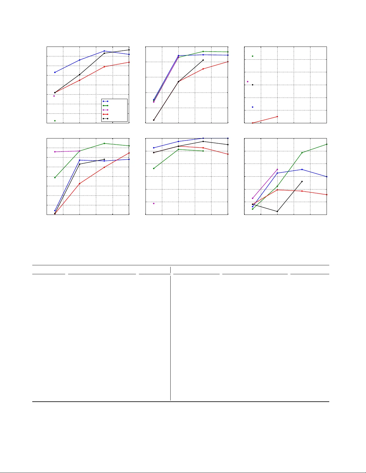
A Subsequence Interlea ving Model f or Sequential P attern Mining Jarosla v F o wkes Charles Sutton School of Inf ormatics University of Edinb urgh, Edinburgh, EH8 9AB, UK {jf owk es, csutton}@ed.ac.uk ABSTRA CT Recen t sequen tial pattern mining methods ha ve used the minim um description length (MDL) principle to define an enco ding scheme which describes an algorithm for mining the most compressing patterns in a database. W e present a no vel subsequence interlea ving mo del based on a probabilis- tic mo del of the sequence database, which allo ws us to search for the most compressing set of patterns without designing a sp ecific enco ding scheme. Our prop osed algorithm is able to efficiently mine the most relev an t sequential patterns and rank them using an asso ciated measure of interestingness. The efficien t inference in our model is a direct result of our use of a structural exp ectation-maximization framework, in whic h the exp ectation-step tak es the form of a submo du- lar optimization problem sub ject to a cov erage constrain t. W e show on both synthetic and real world datasets that our mo del mines a set of sequential patterns with low spurious- ness and redundancy , high interpretabilit y and usefulness in real-w orld applications. F urthermore, w e demonstrate that the quality of the patterns from our approac h is comparable to, if not better than, existing state of the art sequential pattern mining algorithms. 1. INTR ODUCTION Sequen tial data p ose a challenge to exploratory data anal- ysis, as large data sets of sequences are difficult to visualise. In applications such as healthcare (patterns in patient paths [10]), click streams (web usage mining [18]), bioinformatics (predicting protein sequence function [27]) and source code (API call patterns [30]), a common approac h has been se- quential p attern mining , to iden tify a set of patterns that commonly occur as subsequences of the sequences in the data. A natural family of approaches for sequen tial pattern min- ing is to mine frequen t subsequences [2] or closed frequent subsequences [26], but these suffer from the w ell-kno wn prob- lem of pattern explosion, that is, the list of frequent subse- quences is typically long, highly redundant, and difficult to understand. Recen tly , researchers hav e in troduced metho ds to preven t the problem of pattern explosion based on the minimum description length (MDL) principle [12, 25]. These metho ds define an enco ding scheme whic h describ es an al- gorithm for compressing a sequence database based on a library of subsequence patterns, and then search for a set of patterns that lead to the best compression of the database. These MDL metho ds provide a theoretically principled ap- proac h that results in better patterns than frequent subse- quence mining, but their p erformance relies on designing a co ding sc heme. In this pap er, we introduce an alternate probabilistic p er- sp ectiv e on subsequence mining, in whic h we develop a gen- erativ e model of the database conditioned on the patterns. Then, following Shannon’s theorem, the length of the op- timal co de for the database under the model is simply the negativ e logarithm of its probability . This allows us to search for the set of patterns that b est compress the database with- out designing a sp ecific co ding scheme. Our approach, which w e call the Inter esting Se quenc e Miner (ISM) 1 , is a nov el se- quen tial pattern mining algorithm that is able to efficien tly mine the most relev an t sequential patterns from a database and rank them using an associated measure of interesting- ness. ISM mak es use of a no v el probabilistic model of se- quences, based on generating a sequence by in terlea ving a group of subsequences. It is these learned comp onent subse- quences that are the patterns ISM returns. An approach based on probabilistic machine learning brings a v ariet y of b enefits, namely , that the probabilistic mo del al- lo ws us to declaratively incorp orate ideas ab out what types of patterns w ould b e most useful; that we can easily com- p ose the ISM mo del with other types of probabilistic mo dels from the literature; and that w e are able to bring to b ear p o w erful to ols for inference and optimization from proba- bilistic mac hine learning. Inference in our model inv olves appro ximate optimization of a non-monotone submo dular ob jectiv e subject to a submo dular cov erage constraint. The necessary partition function is in tractable to construct di- rectly , how ev er w e show that it can b e efficiently computed using a suitable low er bound. The set of sequential patterns under our mo del can b e inferred efficiently using a structur al exp e ctation maximization (EM) framework [8]. This is, to our kno wledge, the first use of an exp ectation-maximization sc heme for the subsequence mining problem. On real-w orld datasets (Section 4), we find that ISM re- turns a notably more div erse set of patterns than the recent MDL metho ds SQS and GoKrimp (T able 2), while retain- ing similar qualit y . A more div erse set of patterns is, w e suggest, esp ecially suitable for manual examination during exploratory data analysis. Qualitativ ely , the mined patterns from ISM are all highly correlated and extremely relev an t, e.g. represen ting phrases such as oh de ar or concepts suc h as r epr o ducing kernel hilb ert sp ac e . More broadly , this new p er- sp ectiv e has the p otential to op en up a wide v ariety of future directions for new mo delling approac hes, such as com bining sequen tial pattern mining methods with hierarchical mo dels, topic models, and nonparametric Bay esian metho ds. 1 h ttps://github.com/mast-group/sequence-mining 1 2. RELA TED W ORK Sequen tial pattern mining w as first introduced by Agraw al and Srikan t [2] in the context of mark et bask et analysis, whic h led to a num b er of other algorithms for frequent sub- sequence, including GSP [23], PrefixSpan [22], SP ADE [29], and SP AM [3]. F requent sequence mining suffers from p at- tern explosion : a huge num b er of highly redundant frequen t sequences are retrieved if the given minimum supp ort thresh- old is to o low. One wa y to address this is by mining frequen t closed sequences, i.e., those that hav e no subsequences with the same frequency , such as via the BIDE algorithm [26]. Ho wev er, ev en mining frequent closed sequences does not fully resolv e the problem of pattern explosion. W e refer the in terested reader to Chapter 11 of [1] for a survey of frequent sequence mining algorithms. In an attempt to tackle this problem, mo dern approaches to sequence mining ha ve used the minimum description length (MDL) principle to find the set of sequences that b est sum- marize the data. The GoKrimp algorithm [12] directly mines sequences that b est compress a database using a MDL-based approac h. The goal of GoKrimp is essentially to co v er the database with as few sequences as p ossible, because the dictionary-based description length that is used b y GoKrimp fa vours enco ding schemes that cov er more long and frequen t subsequences in the database. In fact, finding the most com- pressing sequence in the database is strongly related to the maxim um tiling problem, i.e., finding the tile with largest area in a binary transaction database. SQS-Searc h (SQS) [25] also uses MDL to find the set of sequences that summarize the data best: a small set of in- formativ e sequences that ac hieve the best compression is mined directly from the database. SQS uses an encoding sc heme that explicitly punishes gaps b y assigning zero cost for enco ding non-gaps and higher cost for enco ding larger gaps b etw een items in a pattern. While SQS can b e very effectiv e at mining informative patterns from text, it can- not handle interlea ving patterns, unlike GoKrimp and ISM, whic h can b e a significan t dra wback on certain datasets e.g. patterns generated by indep endent pro cesses that may fre- quen tly o v erlap. In related work, Mannila and Meek [15] prop osed a gener- ativ e mo del of sequences whic h finds partial orders that de- scrib e the ordering relationships betw een items in a sequence database. Sequences are generated b y selecting a subset of items from a partial order with a learned inclusion probabil- it y and arranging them into a compatible random ordering. Unlik e ISM, their model does not allo w gaps in the gener- ated sequences and each sequence is only generated from a single partial order, an unrealistic assumption in practice. There has also b een some existing research on probabilis- tic mo dels for sequences, esp ecially using Mark ov models. Gw adera et al. [9] use a v ariable order Marko v mo del to iden- tify statistically significant sequences. Stolc k e and Omohun- dro [24] developed a structure learning algorithm for HMMs that learns b oth the num b er of states and the top ology . Landw ehr [13] extended HMMs to handle a fixed num b er of hidden pro cesses whose outputs interlea ve to form a se- quence. W oo d et al. developed the sequence memoizer [28], a v ariable order Mark o v mo del with a Pitman-Y or pro cess prior. Also, Nevill-Manning and Witten [20] infer a con text- free grammar o v er sequences using the Sequitur algorithm. 3. MINING SEQUENTIAL P A TTERNS In this section we will formulate the problem of identifying a set of in teresting sequences that are useful for explaining a sequence database. First we will define some preliminary concepts and notation. An item i is an element of a uni- v erse U = { 1 , 2 , . . . , n } that indexes symbols. A se quenc e S is simply an ordered list of items ( e 1 , . . . , e m ) such that e i ∈ U ∀ i . A sequence S a = ( a 1 , . . . , a n ) is a subsequence of another sequence S b = ( b 1 , . . . , b m ) , denoted S a ⊂ S b , if there exist integers 1 ≤ i 1 < i 2 < . . . < i n ≤ m such that a 1 = b i 1 , a 2 = b i 2 , . . . , a n = b i n (i.e., the standard definition of a subsequence). A sequence datab ase is merely a list of sequences X ( j ) . F urther, we say that a sequence S is sup- p orte d by a sequence X in the sequence database if S ⊂ X . Note that in the abov e definition eac h sequence only con- tains a single item as this is the most imp ortant and p op- ular sequence type (cf. w ord sequences, protein sequences, clic k streams, etc.). 2 A multiset M is a generalization of a set that allo ws elements to o ccur multiple times, i.e., with a sp ecific multiplicity # M ( · ) . F or example in the m ultiset M = { a, a, b } , the elemen t a o ccurs twice and so has m ulti- plicit y # M ( a ) = 2 . 3.1 Problem F ormulation Our aim in this work is to infer a set of interesting sub- sequences I from a database of sequences X (1) , . . . , X ( N ) . Here by inter esting , we mean a set of patterns that are use- ful for helping a human analyst to understand the imp ortan t prop erties of the database, that is, interesting subsequences should reflect the most imp ortant patterns in the data, while b eing sufficiently concise and non-redundant that they are suitable for manual examination. These criteria are inher- en tly qualitativ e, reflecting the fact that the goal of data mining is to build human insigh t and understanding. T o quan tify these criteria, we op erationalize the notion of inter- esting sequence as those sequences that b est explain the un- derlying database under a prob abilistic mo del of sequences. Sp ecifically we will use a gener ative mo del, i.e., a mo del that starts with a set of interesting subsequences I and from this set generates the sequence database X (1) , . . . , X ( N ) . Our goal is then to infer the most likely generating set I un- der our c hosen generativ e mo del. W e wan t a mo del that is as simple as p ossible yet p ow erful enough to capture cor- relations betw een items in sequences. A simple such mo del is as follows: iteratively sample subsequences S from I and randomly interlea v e them to form the database sequence X . If we associate eac h subsequence S ∈ I with a probabilit y π S , we can sample the indicator v ariable z S ∼ Bernoulli ( π S ) and include it in X if z S = 1 . How ev er, we ma y wish to in- clude a subsequence more than once in the sequence X , that is, we need some wa y of sampling the multiplicit y of S in X . The simplest w ay to do this is to change our generating dis- tribution from Bernoulli to e.g. Categorical and sample the m ultiplicity z S ∼ Categorical ( π S ) where π S is now a vec- tor of probabilities, with one entry for each multiplicit y (up to the maximum in the database). W e define the generative mo del formally in the next section. 3.2 Generative Model 2 Note that we can easily extend our algorithm to mine se- quences of sets of items (as defined in the original sequence mining pap er [2]) by extending the subsequence op erator ⊂ to handle these more general ‘sequences’ . 2 As discussed in the previous section, w e prop ose a simple directed graphical mo del for generat ing a database of se- quences X (1) , . . . , X ( N ) from a set I of interesting sequences. The generativ e story for our mo del is, indep endently for each sequence X in the database: 1. F or each in teresting sequence S ∈ I , decide indep en- den tly the n umber of times S should b e included in X , i.e., sample the multiplicit y z S ∈ N 0 as z S ∼ Categorical ( π S ) , where π S is a v ector of multiplicit y probabilities. F or clar- it y w e present the Categorical distribution here but one could use a more general distribution if desired. 2. Set S to b e the multiset with multiplicities z S of all the sequences S selected for inclusion in X : S : = { S | z S ≥ 1 } . 3. Set P to b e the set of all possible sequences that can b e generated by interlea ving together all o ccurrences of the sequences in the multiset S , i.e., P : = { X | S partition of X, S ⊂ X ∀ S ∈ S } . Here b y interle aving we mean the placing of items from one sequence in to the gaps b etw een items in another whilst main taining the orders of the items imp osed b y eac h sequence. 4. Sample X uniformly from P , i.e., X ∼ P . Note that we nev er need to construct the set P in practice, since we only require its cardinalit y during inference, and w e show in the next section how w e can efficiently compute an appro ximation to |P | . W e can, how ever, sample from P efficien tly b y merging subsequences S ∈ S into X one at a time as follows: splice the elements of S , in order, into X at randomly c hosen points (here by splicing S in to X w e mean the placing of items from S into the gaps betw een items in X ). F or example, S = { (1 , 2) , (3 , 4) } will generate the set of sequences P = { (3 , 4 , 1 , 2) , (3 , 1 , 4 , 2) , (3 , 1 , 2 , 4) , (1 , 3 , 4 , 2) , (1 , 3 , 2 , 4) , (1 , 2 , 3 , 4) } . W e could of course learn a transi- tion distribution b etw een subsequences in our model, but w e choose not to do so b ecause we wan t to force the model to use I to explain the sequen tial dep endencies in the data. 3.3 Inference Giv en a set of in teresting sequences I , let z denote the v ector of z S for all sequences S ∈ I and similarly , let Π denote the list of π S for all S ∈ I . Assuming z , Π are fully determined, it is evident from the generative mo del that the probabilit y of generating a database sequence X is p ( X, z | Π ) =  1 |P | Q S ∈I Q | π S |− 1 m =0 π [ z S = m ] S m if X ∈ P , 0 otherwise , where | π S | is the length of π S and [ z S = m ] ev aluates to 1 if z S = m , 0 otherwise. In tuitively , it helps to think of eac h π S as b eing an infinite vector and eac h S ∈ I as being augmen ted with a Kleene star operator, so that, for exam- ple, one can use (1 , 2) ∗ and (3) ∗ to generate the sequence (1 , 2 , 1 , 3 , 2) . Calculating the normalization constan t |P | is problem- atic as w e ha ve to coun t the n um ber of possible distinct sequences that could b e generated by interlea ving together subsequences in S . This is further complicated b y the fact that S is a m ultiset and so can con tain multiple o ccurrences of the same subsequence, whic h mak es efficien t computa- tion of |P | impractical. How ever, it turns out that we can compute a straightforw ard upper b ound since |P | is clearly b ounded ab ov e b y all p ossible p ermutations of all the items in all the subsequences S ∈ S , and this b ound is attained when S contains only distinct singleton sequences without rep etition. F ormally , |P | ≤  P S ∈S | S |  ! Con venien tly , this gives us a non-trivial low er-b ound on the p osterior p ( X , z | Π ) which, as we will w an t to maximize the p osterior, is precisely what w e w ant. Moreo v er, the low er b ound acts as an additional penalty , strongly fa vouring a non-redundan t set of sequences (see Section 4.2). No w assuming the parameters Π are known, we can infer z for a database sequence X b y maximizing the log of the lo wer b ound on the posterior p ( X , z | Π ) ov er z : max z X S ∈I | π S |− 1 X m =0 [ z S = m ] ln( π S m ) − P S ∈S | S | X j =1 ln j s.t. X ∈ P . (3.1) This is an NP-hard problem in general and so impractical to solv e directly in practice. Ho w ev er, w e will sho w that it can b e viewed as a sp ecial case of maximizing a submo dular function sub ject to a submo dular constraint and so appro x- imately solv ed using the greedy algorithm for submo dular function optimization. Now strictly speaking the notion of a submo dular function is only applicable to sets, how ev er we will consider the following generalization to multisets: Definition 1. (Submo dular Multiset F unction) Let Ω be a finite multiset and let N 0 Ω denote the set of all possible m ultisets that are subsets of Ω , then a function f : N 0 Ω → R is submo dular if for for ev ery C ⊂ D ⊂ Ω and S ∈ Ω with # C ( S ) = # D ( S ) it holds that f ( C ∪ { S } ) − f ( C ) ≥ f ( D ∪ { S } ) − f ( D ) . Let us no w define a function f for our sp ecific case: let T b e the m ultiset of supported in teresting sequences, i.e., sequences S ∈ I s.t. S ⊂ X with multiplicit y given b y the maxim um num ber of o ccurrences of S in any partition of X . No w, define f : N 0 T → R as f ( C ) : = X S ∈C | π S |− 1 X m =0 [# C ( S ) = m ] ln( π S m ) − P S ∈C | S | X j =1 ln j and g ( C ) : = |∪ S ∈C S | . W e can no w re-state (3.1) as: Find a non-ov erlapping multiset cov ering C ⊂ T that maximizes f ( C ) , i.e., suc h that g ( C ) = g ( T ) and f ( C ) is maximized. Note that g ( T ) = | X | by construction. No w clearly g is monotone submo dular as it is a m ultiset co v erage function, and we will show that f is non-monotone submodular. T o see that f is submodular observe that for C ⊂ D , # C ( S ) = 3 # D ( S ) f ( D ∪ { S } ) − f ( D ) = ln( π S # D ( S )+1 ) − ln( π S # D ( S ) ) − P D ∈D | D | + | S | X j = P D ∈D | D | +1 ln j ≤ ln( π S # C ( S )+1 ) − ln( π S # C ( S ) ) − P C ∈C | C | + | S | X j = P C ∈C | C | +1 ln j = f ( C ∪ { S } ) − f ( C ) whic h is precisely Definition 1. T o see that f is non-monotone observ e that f ( C ∪ { S } ) − f ( C ) = ln  π S # C ( S )+1 π S # C ( S )  − P C ∈C | C | + | S | X j = P C ∈C | C | +1 ln j whose sign is indeterminate. Maximizing the posterior (3.1) is therefore a problem of maximizing a submo dular function subject to a submodular co verage constraint and can b e appro ximately solv ed b y ap- plying the greedy appro ximation algorithm (Algorithm 1). The greedy algorithm builds a multiset cov ering C by re- p eatedly c ho osing a sequence S that maximizes the profit f ( C ∪ { S } ) − f ( C ) of adding S to the co v ering divided b y the n um ber of items in S not y et co vered b y the cov ering g ( C ∪ { S } ) − g ( C ) = | S | . In order to minimize CPU time sp ent solving the problem, w e cac he the sequences and cov erings for eac h database sequence as needed. Algorithm 1 Greedy Algorithm Input: Database sequence X , supported sequences T Initialize m ultiset C ← ∅ while g ( C ) 6 = | X | do Cho ose S ∈ T maximizing f ( C ∪{ S } ) − f ( C ) | S | C ← C ∪ { S } end while return C Note that while there are go o d theoretical guaran tees on the appro ximation ratio ac hiev ed b y the greedy algorithm when maximizing a monotone submo dular set function sub- ject to a co v erage constraint (e.g. ln | X | + 1 for w eighted set co ver [5, 7]) the problem of maximizing a non-monotone submo dular set function sub ject to a co verage constrain t has, to the b est of our knowledge, not been studied in the literature. How ever, as our submo dular optimization prob- lem is an extension of the w eigh ted set cov er problem, the greedy algorithm is a natural fit and indeed we observe go o d p erformance in practice. 3.4 Learning Giv en a set of in teresting sequences I , consider no w the case where b oth v ariables z , Π in the mo del are unknown. In this case w e can use the hard EM algorithm [6] for parame- ter estimation with laten t v ariables. The hard-EM algorithm in our case is merely a simple lay er on top of the inference Algorithm 2 Hard-EM Input: Set of sequences I and initial estimates Π (0) k ← 0 do k ← k + 1 E-step: ∀ X ( i ) solv e (3.1) to get z ( i ) S ∀ S ∈ T i M-step: π ( k ) S m ← 1 N P N i =1 [ z ( i ) S = m ] ∀ S ∈ I , ∀ m while k Π ( k − 1) − Π ( k ) k F > ε Remo ve from I sequences S with π S 0 = 1 return I , Π ( k ) algorithm (3.1). Suppose there are N database sequences X (1) , . . . , X ( N ) with multisets of supported interesting se- quences T (1) , . . . , T ( N ) , then the hard EM algorithm is given in Algorithm 2 (note that k·k F denotes the F rob enius norm and π S 0 is the probability that S do es not explain an y se- quence in the database). T o initialize Π , a natural c hoice is simply the support (relative frequency) of each sequence. 3.5 Inferring new sequences W e infer new sequences using structural EM [8], i.e., we add a candidate sequence S 0 to I if doing so improv es the optimal v alue p of the problem (3.1) av eraged across all database sequences. Interestingly , there are tw o implicit reg- ularization effects here. Firstly , observe from (3.1) that when a new candidate S 0 is added to the model, a corresp onding term ln π S 0 0 is added to the log-lik elihoo d of all database se- quences that S 0 do es not supp ort. F or large sequence databases, this amounts to a significan t p enalty on candidates in prac- tice. Secondly , observ e that the last term of (3.1) acts as an additional p enalty , strongly fav ouring a non-redundant set of sequences. T o get an estimate of maximum b enefit to including can- didate S 0 , we m ust carefully choose an initial v alue of π S 0 that is not to o lo w, to av oid getting stuc k in a local opti- m um. T o infer a goo d π S 0 , w e force the candidate S 0 to explain all database sequences it supports b y initializing π S 0 = (0 , 1 , . . . , 1) T and update π S 0 with the probability corresp onding to its actual usage once we hav e inferred all the cov erings. Given a set of interesting sequences I and cor- resp onding probabilities Π along with database sequences X (1) , . . . , X ( N ) , eac h iteration of the structural EM algo- rithm is giv en in Algorithm 3 b elow. Occasionally the Hard-EM algorithm may assign zero probabilit y to one or more singleton sequences and cause the greedy algorithm to not b e able to fully cov er a database sequence X using just the in teresting sequences in I . In this case we simply re-seed I with the necessary singletons. Fi- nally , in practice w e store the set of candidates that ha v e b een rejected b y Structural-EM and chec k eac h poten- tial candidate against this set for efficiency . 3.6 Candidate generation The Structural-EM algorithm (Algorithm 3) requires a metho d to generate new candidate sequences S 0 that are to b e considered for inclusion in the set of interesting sequences I . One possibility w ould be to use the GSP algorithm [23] to recursiv ely suggest larger sequences starting from single- tons, ho w ev er preliminary experiments found this was not the most efficien t method. F or this reason w e tak e a sligh tly differen t approach and recursively com bine the in teresting 4 Algorithm 3 Structural-EM (one iteration) Input: Sequences I , Π , optima p ( i ) of (3.1) ∀ X ( i ) Set profit p ← 1 N P N i =1 p ( i ) do Generate candidate S 0 using Candida te-Gen I ← I ∪ { S 0 } , π S 0 ← (0 , 1 , . . . , 1) T E-step: ∀ X ( i ) solv e (3.1) to get z ( i ) S ∀ S ∈ T i M-step: π 0 S m ← 1 N P N i =1 [ z ( i ) S = m ] ∀ S ∈ I , ∀ m ∀ X ( i ) , solv e (3.1) using π 0 S , z ( i ) S ∀ S ∈ T i to get the optimum p ( i ) Set new profit p 0 ← 1 N P N i =1 p ( i ) I ← I \ { S 0 } while p 0 ≤ p {until one go o d candidate found} I ← I ∪ { S 0 } return I , Π 0 sequences in I with the highest supp ort first (Algorithm 4). In this w ay our candidate generation algorithm is more likely to prop ose viable candidate sequences earlier and in practice w e find that this heuristic works well. Algorithm 4 Candida te-Gen Input: Sequences I , cached supports σ , queue length q if @ priority queue Q for I then Initialize σ -ordered priorit y queue Q Sort I by decreasing sequence supp ort using σ for all ordered pairs S 1 , S 2 ∈ I , highest ranked first do Generate candidate S 0 = S 1 S 2 Cac he support of S 0 in σ and add S 0 to Q if |Q| = q break end for end if Pull highest-rank ed candidate S 0 from Q return S 0 3.7 Mining Interesting Sequences Our complete in teresting sequence mining (ISM) algo- rithm is given in Algorithm 5. Note that the Hard-EM pa- Algorithm 5 ISM (Interesting Sequence Miner) Input: Database of sequences X (1) , . . . , X ( N ) Initialize I with singletons, Π with their supp orts while not con v erged do A dd sequences to I , Π using Structural-EM Optimize parameters for I , Π using Hard-EM end while return I , Π rameter optimization step need not be performed at every iteration, in fact it is more efficient to suggest sev eral can- didate sequences b efore optimizing the parameters. As all op erations on database sequences in our algorithm are triv- ially parallelizable, we p erform the E and M -steps in b oth the hard and structural EM algorithms in parallel. 3.8 Interestingness Measur e No w that we ha ve inferred the mo del v ariables z , Π , we are able to use them to rank the retrieved sequences in I . There are tw o natural rankings one can employ , and both ha ve their strengths and weaknesses. The obvious approach is to rank each sequence S ∈ I according to its probabil- it y under the model π S , how ever this has the disadv an tage of strongly fa v ouring frequen t sequences o v er rare ones, an issue we w ould like to av oid. An alternative is to rank the retriev ed sequences according to their inter estingness under the mo del, that is the ratio of database sequences they ex- plain to database sequences they support. One can think of in terestingness as a measure of ho w necessary the sequence is to the mo del: the higher the interestingness, the more sup- p orted database sequences the sequence explains. Thus in- terestingness pro vides a more balanced measure than prob- abilit y , at the expense of missing some frequen t sequences that only explain some of the database sequences they sup- p ort. W e define interestingness formally as follows. Definition 2. The inter estingness of a sequence S ∈ I re- triev ed b y ISM (Algorithm 5) is defined as int ( S ) = P N i =1 [ z ( i ) S ≥ 1] supp ( S ) and ranges from 0 (least interesting) to 1 (most interesting). An y ties in the ranking can b e broken using the sequence probabilit y p ( S ⊂ X ) = p ( z S ≥ 1) = 1 − π S 0 . 3.9 Correspondence to Existing Models There is a close and well-kno wn connection betw een prob- abilistic mo delling and the minimum description length prin- ciple used by SQS and GoKrimp (see MacKay [14], §28.3 for a particularly nice explanation). Given a probabilistic mo del p ( X | Π , I ) of a single database sequence X , by Shannon’s theorem the optimal code for the mo del will enco de X us- ing appro ximately − log 2 p ( X | Π , I ) bits. So b y finding a set of patterns that maximizes the probability of the data, we are also finding patterns that minimize description length. Con versely , any encoding scheme implicitly defines a prob- abilistic mo del. Given an enco ding scheme E that assigns eac h database sequence X to a string of L ( X ) bits, w e can define p ( X | E ) ∝ 2 − L ( X ) , and then E is an optimal code for p ( X | E ) . In terpreting the previous subsequence mining metho ds in terms of their implicit probabilistic mo dels pro- vides in teresting insigh ts into these methods. The enco ding of a database sequence used by SQS can b e in terpreted as a probabilistic model p ( X, z | Π , I ) , where the SQS analog of p ( X , z | Π , I ) is similar to (3.1) with π S m = P N i =1 z ( i ) S P I ∈I P N j =1 z ( j ) I ! m , along with additional terms that corresp ond to the descrip- tion lengths for indicating the presence and absence of gaps in the usage of a sequence S . A dditionally , SQS contains an explicit p enalty for the enco ding of the set of patterns I , that encourages a smaller num b er of patterns. In a proba- bilistic mo del, this can b e interpreted as a prior distribution p ( I ) ov er patterns. There is also a prior distribution on the con tent of the patterns, similar to a unigram model, whic h encourages the patterns to contain more common elements. 5 Similarly , GoKrimp uses a v arian t of the abov e mo del, where instead w e hav e π S m = P N i =1 z ( i ) S + |{ T ∈ I | S ⊂ T }| P I ∈I P N j =1 z ( j ) I + |{ T ∈ I | I ⊂ T }| ! m . In addition, the description length used by GoKrimp also has a gap cost that penalizes sequences with large gaps. GoKrimp employs a greedy heuristic to find the most com- pressing sequence: an empt y sequence S is iterativ ely ex- tended by the most frequen t item that is statistically dep en- den t on S . ISM, b y contrast, iterativ ely extends sequences b y the most frequent sequence in its candidate generation step whic h enables it to quic kly generate large candidate sequences (Section 3.6). W e did consider p erforming a sta- tistical test betw een a sequence and its extending sequence, ho wev er this prov ed computationally prohibitive. The differences betw een these mo dels and ISM are: • Interle aving. SQS cannot mine subsequences that are in- terlea ved and thus struggles on datasets whic h consist mainly of in terleav ed subsequences (for illustration, see Section 4.4). GoKrimp handles in terlea ving using a pointer sc heme that explicitly enco des the location of the subse- quence within the database. In ISM, the partition function |P | allows us to handle in terlea ving of subsequences with- out needing to explicitly encode p ositions, and also serves as an additional p enalty on the num ber of elements in the subsequences used to explain a database sequence. • Gap p enalties. Both SQS and GoKrimp explicitly pun- ish gaps in sequen tial patterns. A dding suc h a penalty w ould require only a trivial mo dification to the algorithm, namely , up dating the cost function in Algorithm 1. W e did not pursue this as we observe excellen t results without it (Section 4). • Enc o ding the set of p atterns. Both SQS and GoKrimp con- tain an explicit p enalty term for the description length of the pattern database, which corresp onds to a prior distri- bution p ( I ) o v er patterns. In our experiments with ISM, w e did not find in practice that an explicit prior distri- bution p ( I ) w as necessary for go o d results. It would b e p ossible to incorp orate it with a trivial change to the ISM algorithm, in particular, when computing the score im- pro vemen t of a new candidate in the structural EM step. • Enc o ding p attern absenc e. Also, observ e that, if we view ISM as an MDL-t ype metho d, not only the presence of a pattern, but also the absence of it is explicitly enco ded (in the form of π S 0 in (3.1)). As a result, there is an implicit p enalt y for adding too man y patterns to the mo del and one do es not need to use a code table which w ould serve as an explicit p enalty for greater mo del complexity . 4. NUMERICAL EXPERIMENTS In this section w e p erform a comprehensiv e quantitativ e and qualitativ e ev aluation of ISM. On syn thetic datasets w e show that ISM returns a list of sequential patterns that is largely non-redundan t, contains few spurious correlations and scales linearly with the num b er of sequences in the dataset. On a set of real-w orld datasets we sho w that ISM finds patterns that are consistent, in terpretable and highly relev ant to the problem at hand. Moreov er, we show that ISM is able to mine patterns that achiev e goo d accuracy when used as binary features for real-world classification tasks. 10 3 10 4 10 5 10 6 No. Sequences 10 1 10 2 10 3 10 4 10 5 Time (s) Figure 1: ISM scaling as the n um ber of sequences in our syn thetic database increases. Datasets W e use ten real-world datasets in our numer- ical ev aluation (see T able 1). The Alice dataset consists of the text of Lewis Carrol’s Alice in W onderland, tokenized in to 1 , 638 sen tences using the Stanford Do cument Prepro- cessor [17] with stop w ords and punctuation delib erately retained. The Gazelle dataset consists of 59 , 601 sequences of clickstream data from an e-commerce website used in the KDD-CUP 2000 competition [11]. The JMLR dataset con- sists of 788 abstracts from the Journal of Machine Learning Researc h and has previously b een used in the ev aluation of the SQS and GoKrimp algorithms [12, 25]. Each sequence is a list of stemmed words from the text with stop w ords re- mo ved. The Sign dataset is a list of 730 American sign lan- guage utterances where each utterance contains a n um ber of gestural and grammatical fields [21]. The last six datasets listed in T able 1 were first in troduced in [19] to ev aluate classification accuracy when mined sequen tial patterns are used as features. The datasets were con v erted from time in- terv al sequences into sequences of items b y considering the start and end of eac h unique interv al as distinct items and ordering the items according to time. ISM R esults W e ran ISM on each dataset for 1 , 000 itera- tions with a priorit y queue size of 100 , 000 candidates. The run time and num b er of non-singleton sequential patterns re- turned by ISM is giv en in the right-hand side of T able 1. W e also in v estigated the scaling of ISM as the num b er of se- quences in the database increases, using the model trained on the Sign dataset from Section 4.1 to generate synthetic sequence databases of v arious sizes. W e ran ISM for 100 it- erations on these databases and one can see in Figure 1 that Dataset Uniq. Items Sequences Subseq. † Run time Alice 2 , 619 1 , 638 123 114 min Gazelle 497 59 , 601 727 582 min JMLR 3 , 846 788 361 230 min Sign 267 730 159 31 min aslbu 250 424 144 4 min aslgt 94 3 , 464 57 19 min auslan2 16 200 10 > 1 min context 94 240 19 7 min pioneer 178 160 86 3 min skating 82 530 70 9 min T able 1: Summary of the real datasets used and ISM results after 1 , 000 iterations. † excluding singleton subsequences. 6 0.0 0.2 0.4 0.6 0.8 1.0 R ecall 0.0 0.2 0.4 0.6 0.8 1.0 Precision ISM SQS GoKrimp BIDE Figure 2: Precision against recall for eac h algorithm on our syn thetic database, using the top- k patterns as a threshold. Note that SQS is a single p oin t at the top-left and GoKrimp has near zero precision and recall. Each plotted curve is the 11-p oin t in terpolated precision 3 . the scaling is linear as exp ected. All experiments were p er- formed on a mac hine with 16 In tel Xeon E5-2650 2 . 60 Ghz CPUs and 128GB of RAM. Evaluation criteria W e will ev aluate ISM along with SQS, GoKrimp and BIDE according to the following criteria: 1. Spuriousness – to assess the degree of spurious correlation in the mined set of sequential patterns. 2. R e dundancy – to measure ho w redundant the mined set of patterns is. 3. Classific ation A c cur acy – to measure the usefulness of the mined patterns. 4. Interpr etability – to informally assess how meaningful and relev ant the mined patterns actually are. 4.1 Patter n Spuriousness The sequence-cov er formulation of the ISM algorithm (3.1) naturally fa v ours adding sequences to the mo del whose items co-o ccur in the sequence database. One would therefore ex- p ect ISM to largely a v oid suggesting sequences of uncor- related items and so return more meaningful patterns. T o v erify this is the case and v alidate our inference pro cedure, w e c heck if ISM is able to reco ver the sequences it used to generate a synthetic database. T o obtain a realistic synthetic database, we sampled 10 , 000 sequences from the ISM gen- erativ e mo del trained on the Sign dataset (cf. Section 3.2). W e were then able to measure the precision and recall for eac h algorithm, i.e., the fraction of mined patterns that are generating and the fraction of generating patterns that are mined, resp ectively . Figure 2 sho ws the precision-recall curv e for ISM, SQS, GoKrimp and BIDE using the top- k mined sequences (according to eac h algorithms ranking) as a threshold. One can clearly see that ISM was able to mine al- most all the generating patterns and almost all the patterns mined w ere generating, despite the fact that the generated database will contain many subsequences not present in the original dataset due to the nature of our ‘subsequence inter- lea ving’ generative mo del. This not only provides a go o d v al- idation of ISM’s inference pro cedure and underlying genera- tiv e model but also demonstrates that ISM returns few spu- rious patterns. F or comparison, SQS returned a very small 3 i.e., the in terpolated precision at 11 equally spaced recall p oin ts b etw een 0 and 1 (inclusive), see [16], §8.4 for details. set of generating patterns and GoKrimp returned man y pat- terns that w ere not generating. The set of top- k patterns mined b y BIDE contained successively less generating pat- terns as k increased. It is not our in tention to draw con- clusions about the performance of the other algorithms as this exp erimental setup naturally fav ours ISM. Instead, w e compare the patterns from ISM with those from SQS and GoKrimp on real-w orld data in the next sections. 4.2 Patter n Redundancy W e now turn our atten tion to ev aluating how redundant the sets of sequen tial patterns returned by ISM, SQS, GoKrimp and BIDE actually are. A suitable measure of redundancy for a single sequence is the minim um edit distance betw een it and the other mined sequences in the set. A v eraging this distance across all sequences in the set, w e obtain the av- er age inter-se quenc e distanc e (ISD). Similarly , w e can also calculate the a v erage n um ber of sequences containing other mined sequences in the set (CS), which provides us with an- other measure of redundancy . Finally , we can also lo ok at the num ber of unique items presen t in the set of mined se- quences which gives us an indication of how diverse it is. W e ran ISM, SQS, GoKrimp and BIDE on all the datasets in T able 1 and rep ort the results of the three aforementioned redundancy metrics on the top 50 non-singleton sequential patterns for eac h algorithm in T able 2. One can see that on a verage the top ISM sequences hav e a larger inter-sequence distance, smaller num b er of containing sequences and larger n umber of unique items, clearly demonstrating they are less redundan t than SQS, GoKrimp and BIDE. Predictably , the top BIDE sequences are the most redundant, with an av er- age in ter-sequence distance of 1 . 00 . 4.3 Classification Accuracy A key prop ert y of an y set of patterns mined from data is its usefulness in real-w orld applications. T o this end, in k eeping with previous work [12], w e will focus on classifi- cation tasks as they are some of most imp ortant applica- tions of pattern mining algorithms. Sp ecifically we will con- sider the task of classifying sequences in a database using mined sequential patterns as binary features. W e therefore p erformed 10 -fold cross v alidation using a Supp ort V ector Mac hine (SVM) classifier on the six classification datasets from T able 1 with the top- k patterns mined by ISM, SQS, GoKrimp and BIDE as features. W e used the linear clas- sifier from the libSVM library [4] with default parameters. A dditionally , w e used the top- k most frequent singleton pat- terns as a baseline for the classification tasks. The resulting plots of k against classification accuracy for all the datasets and algorithms are given in Figure 3. One can see that the patterns mined by SQS perform b est, exhibiting the highest classification accuracy on four out of the six datasets, closely follo wed by ISM and GoKrimp, which p erforms surprisingly w ell considering it struggles to return more than 50 patterns. All three consistently outperform BIDE and the singletons baseline whic h exhibit similar performance to each other. W e therefore conclude that the sequential patterns mined b y ISM can indeed b e useful in real-world applications. 4.4 Patter n Interpr etability F or the tw o text datasets in T able 1 we can directly in- terpret the mined patterns and informally assess ho w mean- ingful and relev ant they are. 7 Alice Gazelle JMLR Sign aslbu ISD CS Items ISD CS Items ISD CS Items ISD CS Items ISD CS Items ISM 2 . 00 0 . 00 94 3 . 36 0 . 00 167 1 . 84 0 . 00 96 3 . 64 0 . 00 113 2 . 24 0 . 00 110 SQS 1 . 76 0 . 10 72 4 . 24 0 . 38 183 1 . 82 0 . 02 92 1 . 26 0 . 94 57 * 1 . 89 * 0 . 11 * 61 GoKrimp 1 . 24 0 . 10 52 * 4 . 51 * 0 . 05 * 176 * 1 . 40 * 0 . 10 * 30 1 . 72 0 . 24 63 * 2 . 00 * 0 . 00 * 18 BIDE 1 . 00 0 . 36 29 1 . 00 0 . 36 26 1 . 00 0 . 18 12 1 . 00 0 . 60 15 1 . 00 0 . 00 26 aslgt auslan2 context pioneer skating ISD CS Items ISD CS Items ISD CS Items ISD CS Items ISD CS Items ISM 2 . 08 0 . 20 94 * 2 . 40 * 1 . 0 * 14 * 2 . 16 * 0 . 47 * 35 2 . 04 0 . 00 102 2 . 12 0 . 72 73 SQS 1 . 96 0 . 28 86 * 1 . 42 * 1 . 17 * 12 2 . 14 0 . 90 64 1 . 64 0 . 40 78 1 . 62 0 . 84 46 GoKrimp * 2 . 00 * 0 . 00 * 89 * 2 . 00 * 0 . 25 * 8 * 2 . 07 * 0 . 52 * 51 * 1 . 82 * 0 . 00 * 33 * 1 . 90 * 0 . 29 * 64 BIDE 1 . 00 0 . 00 22 * 1 . 00 * 3 . 16 * 6 1 . 00 1 . 72 12 1 . 02 0 . 06 32 1 . 00 1 . 06 17 T able 2: A verage inter-sequence distance (ISD), a verage no. con taining sequences (CS) and no. unique items for the top 50 non-singleton sequences returned by the algorithms from the datasets. Larger in ter-sequence distances and smaller no. con taining sequences indicate less redundancy . * returned less than 50 non-singleton sequences. ISM SQS GoKrimp BIDE supp ort v ector mac hin supp ort v ector mac hin support vector mac hin algorithm algorithm real w orld machin learn mac hin learn learn learn larg scale state art real w orld learn algorithm high dimension data set state art algorithm learn state art ba yesian netw ork high dimension data data first second larg scale repro duc hilbert space learn data repro duc k ernel hilbert space nearest neigh bor exp erimen t result mo del model maxim um lik elihoo d decis tree sup ervis learn problem problem wide rang neural net w ork neural net w ork learn result gene express cross v alid comp on analysi problem algorithm princip compon analysi featur select w ell known metho d method random field graphic model supp ort vector algorithm result maxim um en tropi real w orld base result data set lo w dimension high dimension pap er in v estig learn learn learn blind separ m utual inform data demonstr learn problem wide v arieti sampl size hilb ert space learn metho d acycl graph learn algorithm suc h paper algorithm data turn out princip compon analysi algorithm demonstr learn set mark ov chain logist regress learn result problem learn lea v out mo del select learn experi algorithm algorithm algorithm T able 3: The top tw ent y non-singleton sequences as found by ISM, SQS, GoKrimp and BIDE for the JMLR dataset. JMLR Dataset W e compare the top- 20 non-singleton pat- terns mined by ISM, SQS, GoKrimp and BIDE in T able 3. It is immediately obvious from the table that the BIDE pat- terns are almost exclusiv ely permutations of frequen t items and so uninformativ e. F or this reason w e omit BIDE from consideration on the next dataset. The patterns mined by ISM, SQS and GoKrimp are all v ery informative, contain- ing technical concepts such as supp ort vector machine and commonly used phrases such as state (of the) art . A lic e Dataset W e compare the top tw en t y- 20 non-singleton patterns mined by ISM, SQS and GoKrimp in the first three columns T able 4. This time, one can clearly see that the patterns mined by ISM are considerably more informative. They contain collo cated w ords and phrases such as mo ck turtle and oh de ar , correlated w ords such as as sp oke and off head , as w ell as correlated punctuation such as ( ) and “ ” . Both SQS and GoKrimp on the other hand mine collo- cated words with spurious punctuation and stop words, e.g. prep ending the to nouns and commas to phrases. T o further illustrate this notable difference, w e also show the top- 20 non-singleton patterns that are exclusiv e to each algorithm (i.e., found b y ISM but not SQS/GoKrimp, etc.) in the last three columns of T able 4. One can clearly see that GoKrimp has the least informativ e exclusive patterns, predominantly com binations of stop w ords and punctuation, SQS mostly prep ends and app ends informativ e exclusive patterns with punctuation and stop words, whereas ISM is the only algo- rithm that just returns purely correlated words. Note that SQS in particular struggles to return patterns such as bal- anced paren theses, since it punishes the large gaps b et ween them and cannot handle interlea ving them with the patterns they enclose. Here we can really see the p ow er of the statis- tical model underlying ISM as it is able to discern spurious punctuation from gen uine phrases. Par al lel Dataset Finally , w e consider a syn thetic dataset that demonstrates the ability of ISM to handle interlea v- ing patterns. F ollo wing [12], we generate a synthetic dataset where each item in the sequence is generated by fiv e inde- p enden t parallel pro cesses, i.e., each pro cess i generates one item from a set of five p ossible items { a i , b i , c i , d i , e i } in or- der. In each step, the generator c ho oses i at random and generates an item using process i , until the sequence has length 1 , 000 , 000 . The sequence is then split in to 10 , 000 sequences of length 100 . F or this dataset we kno w that all 8 0 20 40 60 80 100 top k 0.46 0.48 0.50 0.52 0.54 0.56 0.58 0.60 0.62 Classification Accuracy aslbu ISM SQS GoKrimp BIDE Singletons 0 20 40 60 80 100 top k 0.3 0.4 0.5 0.6 0.7 0.8 Classification Accuracy aslgt 0 20 40 60 80 100 top k 0.22 0.24 0.26 0.28 0.30 0.32 0.34 Classification Accuracy auslan2 0 20 40 60 80 100 top k 0.2 0.3 0.4 0.5 0.6 0.7 0.8 0.9 1.0 Classification Accuracy context 0 20 40 60 80 100 top k 0.70 0.75 0.80 0.85 0.90 0.95 1.00 Classification Accuracy pioneer 0 20 40 60 80 100 top k 0.18 0.20 0.22 0.24 0.26 0.28 0.30 Classification Accuracy skating Figure 3: Linear SVM classification accuracy using the top- k sequences returned by eac h algorithm as binary features. ISM sho ws consisten tly goo d p erformance, comparable to SQS and GoKrimp. ISM SQS GoKrimp Exclusiv e ISM Exclusiv e SQS Exc. GoKrimp she herself ! ’ ‘ ’ she herself ? ’ ‘ ’ mo c k turtle , and , and ( ) the mo ck turtle , said . ( ) ? ’ , said . he his the march hare said the . w ent on . ’ mo ck turtle as sp oke * * * * of the . “ ” the mock turtle said the . had bac k , ’ said alice i n’t ’ ca n’t the marc h hare in a just when , you know marc h hare he his * * * * of the . off head it w as alice . lo ok ed at , ’ said alice i n’t ’ she at once the white rabbit what ? had been the queen i ’m oh dear , ’ y ou kno w m ust be , y ou kno w marc h hare never before ; and ‘ ! at last w en t on w ent on join dance she had y ou ? as spoke it was a little migh t well b eau – ootiful so o – o op ! , , , lo oking at the white rabbit ! ’ if ’d i ’v e oh , ! had bac k , ’ alice . suc h thing min ute or t w o i ’ just when ; and to herself ’v e seen there was alice ; off head a little as she do n’t know what ‘ well , , ! she at once i ’m what ? going in to – ’ the . oh dear do n’t you know too muc h in a tone alice , more than she had the queen so on found so o – oop of the e – e – it : nev er before b eau – o otiful so o – o op ! the hatter to ok its , ’ said the king and she T able 4: The top tw en t y non-singleton sequences as found by ISM, SQS and GoKrimp for the Alice dataset as w ell as those found b y ISM but not SQS/GoKrimp, SQS not ISM/GoKrimp and GoKrimp not ISM/SQS. 9 0 10 20 30 40 50 top k 0.0 0.2 0.4 0.6 0.8 1.0 R ecall ISM SQS GoKrimp Figure 4: Recall for eac h algorithm on the synthetic par- allel dataset, using the top- k (first- k for SQS) patterns as a threshold. Note that SQS main tains a recall level of 0 . 6 for the remaining patterns (up to k = 403 , not shown for clarit y). mined sequences con taining a mixture of items from differen t pro cesses are spurious. This enables us to calculate recall, i.e., the fraction of pro cesses presen t in the set of true pat- terns mined b y each algorithm. W e plot the recall for the top- k patterns mined by ISM and GoKrimp in Figure 4 and the first- k patterns mined by SQS (as it was still running after seven days). One can see that while ISM and GoKrimp are able to mine true patterns from all processes, SQS only returns patterns from 3 of the 5 pro cesses. 5. CONCLUSIONS In this pap er, w e hav e taken a probabilistic machine learn- ing approach to the subsequence mining problem. W e pre- sen ted a no v el subsequence in terlea ving model, called the In teresting Sequence Miner, that infers subsequences which b est compress a sequence database without ha ving to de- sign a MDL enco ding sc heme. W e demonstrated the efficacy of our approach on b oth syn thetic and real-w orld datasets, sho wing that ISM returns a more div erse set of patterns than previous approac hes while retaining comparable qual- it y . In the future w e would lik e to extend our approach to the many promising application areas as w ell as considering more adv anced techniques for parallelization. Acknowledgments This work was supported b y the Engineering and Physical Sciences Research Council (grant num ber EP/K024043/1). References [1] C. Aggarw al and J. Han. F r e quent Pattern Mining . Springer, 2014. [2] R. Agra w al and R. Srikant. Mining sequential patterns. In ICDE , pages 3–14, 1995. [3] J. A yres, J. Flannic k, J. Gehrke, and T. Yiu. Sequen tial pattern mining using a bitmap represen tation. In KDD , pages 429–435, 2002. [4] C.-C. Chang and C.-J. Lin. LIBSVM: A library for supp ort vector machines. ACM TIST , 2:27:1–27:27, 2011. http://www.csie.n tu.edu.tw/~cjlin/libsvm. [5] V. Ch v átal. A greedy heuristic for the set-co v ering problem. Math. O.R. , 4(3):233–235, 1979. [6] A. Dempster, N. Laird, and D. Rubin. Maximum likelihoo d from incomplete data via the EM algorithm. Journal of the R oyal Statistic al So ciety: Series B , pages 1–38, 1977. [7] U. F eige. A threshold of ln n for approximating set cover. Journal of the ACM , 45(4):634–652, 1998. [8] N. F riedman. The Bay esian structural EM algorithm. In UAI , pages 129–138, 1998. [9] R. Gw adera, M. J. Atallah, and W. Szpanko wski. Marko v models for identification of significant episo des. In SDM , pages 404–414, 2005. [10] N. Jay , G. Herengt, E. Albuisson, F. Kohler, and A. Napoli. Sequential pattern mining and classification of patient path. In MEDINF O , page 1667, 2004. [11] R. K ohavi, C. E. Brodley , B. F rasca, L. Mason, and Z. Zheng. KDD-Cup 2000 organizers’ rep ort: Peeling the onion. SIGKDD Explor ations Newsletter , 2(2):86–93, 2000. [12] H. T. Lam, F. Mo erchen, D. F radkin, and T. Calders. Mining compressing sequential patterns. Statistical A nalysis and Data Mining , 7(1):34–52, 2014. [13] N. Landw ehr. Modeling interlea v ed hidden pro cesses. In ICML , pages 520–527, 2008. [14] D . J. C. MacKay. Information The ory, Infer enc e, and L earning A lgorithms . Cam bridge Univ ersity Press, 2003. [15] H. Mannila and C. Meek. Global partial orders from sequential data. In KDD , pages 161–168, 2000. [16] C. D. Manning, P . Raghav an, and H. Schütze. Intr o duction to Information Retrieval . Cambridge University Press, 2008. [17] C. D. Manning, M. Surdeanu, J. Bauer, J. Finkel, S. J. Bethard, and D. McClosky . The Stanford CoreNLP natural language pro cessing to olkit. In A CL System Demonstr ations , pages 55–60, 2014. [18] B. Mobasher, H. Dai, T. Luo, and M. Nakagaw a. Using sequential and non-sequential patterns in predictive w eb usage mining tasks. In ICDM , pages 669–672, 2002. [19] F. Moerchen and D. F radkin. Robust mining of time interv als with semi-interv al partial order patterns. In SDM , pages 315–326, 2010. [20] C. G. Nevill-Manning and I. H. Witten. Identifying hierarchical structure in sequences: A linear-time algorithm. Journal of Artificial Intel ligenc e Rese ar ch , 7:67–82, 1997. [21] P . Papapetrou, G. Kollios, S. Sclaroff, and D. Gunopulos. Discov ering frequent arrangemen ts of temp oral interv als. In ICDM , pages 82–89, 2005. [22] J. P ei, J. Han, B. Mortazavi-Asl, H. Pinto, Q. Chen, U. Day al, and M.-C. Hsu. PrefixSpan: Mining sequential patterns efficiently by prefix-pro jected pattern growth. In ICDE , pages 215–224, 2001. [23] R . Srikant and R . Agraw al. Mining sequential patterns: Generalizations and p erformance improv emen ts. In EDBT , pages 3–17, 1996. [24] A. Stolc ke and S. Omoh undro. Hidden Mark o v mo del induction by Bay esian mo del merging. In NIPS , pages 11–18, 1993. [25] N. T atti and J. V reek en. The long and the short of it: summarising even t sequences with serial episo des. In KDD , pages 462–470, 2012. [26] J. W ang and J. Han. BIDE: Efficien t mining of frequent closed sequences. In ICDE , pages 79–90, 2004. [27] M . W ang, X.-Q. Shang, and Z.-H. Li. Sequential pattern mining for protein function prediction. In ADMA , pages 652–658. Springer, 2008. [28] F. W o o d, J. Gasthaus, C. Archam b eau, L. James, and Y. W. T eh. The sequence memoizer. Communic ations of the A CM , 54(2):91–98, 2011. [29] M . J. Zaki. SP ADE: An efficient algorithm for mining frequent sequences. Machine L e arning , 42(1-2):31–60, 2001. [30] H. Zhong, T. Xie, L. Zhang, J. P ei, and H. Mei. MAPO: Mining and recommending API usage patterns. In ECOOP , pages 318–343. 2009. 10