Combining observational and experimental data to find heterogeneous treatment effects

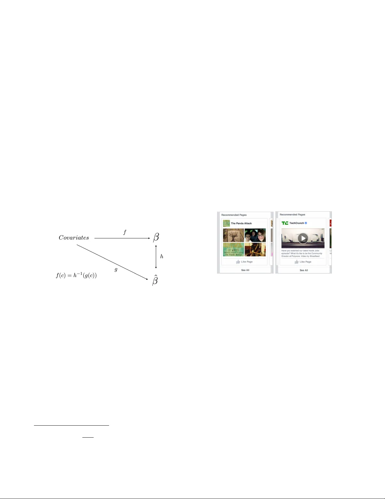
Combining observational and e xperimental data to find heter og eneous treatment effects Ale xander P e ysakhovich F acebook Ar tificial Intelligence Research 770 Broadwa y New Y ork, NY 10003 Akos Lada F acebook News F eed 1 Hack er W ay Menlo P ark, CA 94025 ABSTRA CT Ev ery design c hoice will hav e different effects on differen t units. Ho wev er traditional A/B tests are often underpow- ered to iden tify these heterogeneous effects. This is es- pecially true when the set of unit-level attributes is hi gh- dimensional and our priors are weak ab out whic h particular co v ariates are important. Ho wev er, there are often ob ser- v ational data sets av ailable that are orders of magnitude larger. W e prop ose a metho d to combine these tw o data sources to estimate heterogeneous treatmen t effects. First, w e use observ ational time series data to estimate a map- ping from cov ariates to u nit-level effects. These estimates are likely biased but under some conditions the bias pre- serv es unit-lev el relative rank orderings. If these conditions hold, we only need sufficient exp erimen tal data to identify a monotonic, one-dimensional transformation from observ a- tionally predic ted treatmen t effects to real treatmen t effects. This reduces p ow er demands greatly and makes the detec- tion of heterogeneous effects muc h easier. As an application, w e sho w ho w our method can b e used to impro ve F aceb o ok page recommendations. K eywords Heterogeneous treatment effects; Personalization 1. INTR ODUCTION Experimentation and data-grounded approac hes to the design of pro ducts, websites and services hav e b ecome im- mensely p opular in the internet industry [28, 3]. This is for a very go o d reason: when decision-makers employ exper- imen tation they hav e a far greater chanc e of making go o d decisions than with observ ation alone [22, 4, 2 0, 19, 6]. Stan- dard exp erimentation techniques are often used to ev aluate whether a particular p olicy works on av erage but decision- mak ers and analysts are increasingly in terested in how their designs will affect different groups [13]. Understanding this heterogeneit y is particularly imp ortan t when a design is to o expensive to give to the whole p opulation (and so should Submitted to WWW ’17 P erth, Austr alia A CM ISBN N A. DOI: NA be giv en to the subset that will benefit the most) or when it has positive effects for some, but may not b e appropriate for others. Our con tribution is to discuss how analysts can com bine experimental with observ ational data to help solv e the p ersonalization problem. T raditional metho ds hav e allow ed analysts to sp ecify ex- an te interesting subgroups [13, 17] and look for differences. More modern work in machine learning, statistics and econo- metrics has begun to focus on streamlinin g this process. The methods automatically find heterogeneous groups using a v ariet y of tricks such as non-parametric pro cedures [10, 26], regularized regression [18], trees [14, 25], causal trees and forests [2, 27], deep neural netw orks [24], ‘virtual twin’ anal- yses [11] and mixtures of mo dels [15]. Ho wev er, these automated searches are difficult. In many important domains a verage effects are small (relative to noise), the set of unit-level cov ariates is high-dimensional and we lac k a priori knowledge ab out which cov ariates are imp or- tan t predictors of heterogeneity . The combination of these conditions means that to identify heterogeneous effects pre- cisely exp eriments hav e to b e very large and, in general, prohibitiv ely costly [21]. In contrast to exp ensiv e exp eri- men tal data, observ ational data is often av ailable in muc h larger quantities especially in applications suc h as medicine, online commerce or so cial media. Our contribution is to in- v estigate whether we can combin e this observ ational data with exp eriments to help learn the mapping from unit-level features to heterogeneous effects. Our general approach can b e describ ed by the heuristic “larger correlations suggest larger causal effects.” W e learn a mapping from unit-level cov ariates to the size of the unit- lev el causal effect that we get from using time series observ a- tional data. W e then use this mapping as a rank-preserving transformation of the true causal effects. Of course our heuristic is not alwa ys applicable and we discuss the sta- tistical assumptions on the data generating pro cess under whic h the statement ab ov e is true. Statistical assumptions are useful but often they are ab- stract and so analysts need guidelines for when they are lik ely to hold or not. In general, this requires domain kno wl- edge and reasoning. W e fo cus on a real world application: recommendations of pages to users on F aceb o ok. W e presen t a stylized mo del of user behavior and argue that under rea- sonable assumptions on this behavioral mo del the required statistical assumptions are satisfied. Of course, the final ar- biter of suc h questions is data so we re-analyze an existing product A/B test to show that indeed observ ational data seems to provide a useful prior for exp erimentally estimated causal effects. W e note that our observ ational approach is not in tended to supplant the approac hes su rvey ed abov e. Rather, w e view observ ational data as a complemen t to, not a substitute for, randomized trials. In practice, we suggest that the observ a- tionally predicted treatment effect for eac h unit b e added as a feature into an analyst’s fav orite heterogeneous treatmen t effect pro cedure. There is a cost here: adding another feature raises the complexit y of the machine learning procedure. There is also a b enefit: if the conditions on the data generating pro cesses w e outline here are satisfied the b enefits in predictiv e p ow er ma y b e large. W e argue that if the cov ariate space is already large, the effect on mo del complexity is negligible [12] and so the cost is likely to b e small while the b enefit in terms of reducing exp erimental pow er requiremen ts may b e quite large. 2. THE BASIC SETUP W e work with the following situation: w e ha ve units in- dexed b y i , time indexed by t , a con tinuous v ariable of in- terest x and a contin uous outcome v ariable y . W e hav e a treatmen t whic h can change the v alue of x by one and we are interested in personalizing the cho ice of whether a par- ticular unit (i.e. group or individual) with a given cov ariate profile should or should not receive the treatment (p erhaps the treatment has a cost or finite supply). T o mo del this we assume eac h unit has a linear 1 response: when we raise x i b y one, y will increase by β i . T o complete the mo del, we assume there is a (p otentially high dimen- sional) space of co v ariates C and each unit has a cov ariate profile c i . Note that this cov ariate is assumed fixed per unit and not affected by p olicy choices. There is a (p otentiall y probabilistic) mapping f from co- v ariates to treatmen t effects β i = f ( c i ) and the key to doing goo d p ersonalization is to learn this mapping. One wa y to estimate f is to run a very large exp erimen t. W e can raise x by one unit in treatment (lea ving the control as is) and estimate the function E ( f ( c i )) = E ( y | tr eated, c i ) − E ( y | contr ol, c i ) using off-the-shelf metho ds [26, 18, 14, 25, 2, 27, 24, 11, 15]. Ho wev er, when treatment effects are relatively small and cov ariate space is large this tech nique will require quite large and expensive exp eriments. On the other hand, highly granular observ ational data is often av ailable in large quantit ies in online applications and increasingly also in the domains of medicine and public policy . W e no w discuss ho w to incorporate this observ ational data to help make the pro cess of estimating heterogenous causal effects easier. Suppose that the real data generating pro cess is giv en by the structural equations x t i = θ i +  t i + U t i ψ i and y t i = µ i + x t i β i + U t i γ i + η t i . 1 W e assume linearity b ecause in man y cases of interest our treatmen t will ha ve relativel y small effects on x and thus w e are interested in the locally linear approximation of the true response function. Here we hav e that  and η are error terms indep enden t of all the other v ariables, U is some time v arying unobserved v ariables (whic h in general can be a v ector but for ease of no- tation we write as a scalar quan tity), µ and θ are unobserv ed v ariables that are fixed at the unit level. F or simplicity , all of these v ariables are mean 0 with finite v ariances. Note that this is without loss of generalit y as we could include some observ ed v ariables V t i , then the wa y to apply the method b elow is simply to use not the original x and y but x and y conditional on V (ie. the residuals). F or the rest of this paper w e assume all v ariables other than x and y are unobserv ed b y the analyst. Suppose that for a large set of units i we hav e obser- v ational data for x and y coming from a time series with perio ds t ∈ { 1 , . . . , T } where T is large. Denote each daily data p oint for each unit as ( x t i , y t i ). This is the standard panel data set up, how ever standard panel data techniques are generally in terested in learning the av erage causal effect, not individualized ones [1]. What happ ens if we take this data and run a separate linear regression, including an intercept, for eac h unit? F or simplicit y we assume that T is very large, so we can work with the p opulation quantities free of uncertain ty . First note that the panel asp ect of our data means we can ignore µ i and θ i in the analyses that follo w. This is b ecause E ( x ) = θ i and E ( y ) = µ i + β i µ i . Both of these quantities are fixed within units and thus pick ed up b y the intercept term of eac h unit-specific linear regression. Let us focus on the more interesting question: the co effi- cien t on x in eac h of our unit level regressions. W e will call this our observational ly estimate d ca usal effect ˆ β i . W e don’t observ e U and so our estimated ˆ β i will not be equal to β i due to omitted v ariable bias [1, 6]. W e abuse notation a bit and let X i be demeaned vector of observ ations of x for unit i (similarly for Y i ). Recall that the co efficien t ˆ β i is the solution to the least squares problem ˆ β i = ( X 0 i X i ) − 1 ( X 0 i Y i ) . W e can substitute the structural equation for y (ignoring µ and θ b ecause they hav e b een pick ed up by removing the means) into the abov e to get E ( ˆ β i ) = E (( X 0 i X i ) − 1 ( X 0 i X i β + U i γ i + η i )) whic h after some algebra turns in to E ( ˆ β i ) = β i + E (( X 0 i X i ) − 1 ( X 0 i U i ) γ i ) = β i + C ov ( x i , u i ) V ar ( x i ) γ i where the last step comes from the fact that x and u are scalar. This is an imp ortant example of the difference b etw een prediction problems and in terven tional problems [6], [23]. x i ˆ β i is the b est unbiase d line ar pr e dictor of y i but it is not an estimate of the causal effect β for the same reason that kno wing the num b er of units of ice cream sold on a given da y can predict how many p eople will drown in swimming po ols on that da y but that that banning ice cream (an in ter- v ention) will likely not affect drownings b y nearly as muc h as the observ ational regression would suggest. The bias term here is the quantit y of interest for us. Sup- pose that we ha v e tw o units i , j and we ha v e that β i > β j . If C ov ( x i ,u i ) V ar ( x i ) γ i > C ov ( x j ,u j ) V ar ( x j ) γ j then we are guaran teed to ha ve ˆ β i > ˆ β j . If this condition holds for any such i , j then ˆ β deriv ed from observ ational time series data will b e a rank preserving estimate of β . In other w ords, if “bigger causal ef- fects imply bigger bias” then “larger correlation effects imply larger causation.” 2 In such a case ˆ β i is a sufficient statistic for targeting bud- get constrained in terven tions (ie. when we can only afford to give the in terven tion to some p ercent age of the p opula- tion). This also means that if we can learn a function g whic h maps cov ariates c i to ˆ β i then this function will b e a monotonic transformation of the true heterogeneous effects function f . In practice, we suggest learning g by estimating a set of { ˆ β 1 , . . . , ˆ β N } for a large num b er of units using time series data and then using an y standard machine learning tech- nique to learn E ( ˆ β | c ) . Note that the existence of time series data is what mak e our job here possible because it allows us to remov e time in- v arian t unit-level effects. Without multiple observ ations per unit, it would theoretically b e p ossible to p erform a simi- lar procedure but the assumptions required w ould be muc h stronger as we would need muc h more complex conditions on the co v ariance structure b etw een µ , θ , u and β to hold. Recall that our motiv ation is environmen ts where obser- v ational data is plentiful but exp erimental data is sparse. Th us, if our assumptions ab ov e are satisfied, once we ha ve g we only need to use exp erimental data to learn a one di- mensional transformation h from ˆ β to β rather than the full, high dimensional function f (figure 1). Figure 1: The relationship b etw een the true hetero- geneous treatmen t effect function f and the obser- v ational one g . There is no wa y to chec k whether the assumptions un- derlying our pro cedure hold or not using observ ational data only . How ev er, we are not advocating that observ ational data replace experiments. When analyzing real results, an- alysts will likely already b e using a technique to lo ok for heterogeneous treatment effects using C as a feature space. Our argumen t is simply that the analyst should add ˆ g ( c ) (the unit level predicted v alue of ˆ β ), to the set of unit-lev el features. In the worst case, this increases the complexity of the heterogeneous effect mo del slightly (assuming C is al- ready high dimensional). In the best case, our assumptions hold exactly , ˆ g ( c ) is a p erfect monotonic transformation of f ( c ) and th us using ˆ g ( c ) as a feature greatly reduces exper- imen tal p o wer requirements. 2 Note that this is a sufficien t, but not necessarily condition. It is necessary th at ∂ bias ∂ β > − 1 ho wev er this do esn’t make for as catch y one sentence explanations or as simple to describe behavioral assumptions. 3. APPLICA TION: F A CEBOOK P A GE REC- OMMEND A TIONS W e now w alk through an example where observ ational es- timates can be helpful to analysts interested in understand- ing heterogeneous effects in the real world. W e fo cus on personalization of F aceb o ok’s page recommendation engine. P ages are non-user entities on F aceb o ok than can post con- ten t (e.g. news sites, blogs, certain celebrities). People can ‘Lik e’ a page to connect to it. Liking a page makes p osts that the page creates eligible to app ear in the liker’s News F eed. Helping users connect to conten t they care ab out can greatly improv e their exp erience on the site, therefore F ace- bo ok employs recommendations to suggest relev ant pages to users. These recommendations can sho w up in a user’s News F eed in the form of ‘Pages Y ou May Like’ units (figure 2 for an example). F acilitating these connections has co sts. There is opportu- nit y cost (v arious ‘Recommended Page’ units tak e up space on the News F eed) and there is a related user exp erience cost (users who do not wan t or need more connections can be incon venienced or anno y ed). Thus, unlike in the standard recommender system setting where the question of interest is which p age should we suggest [5], an equally imp ortant question for us to address is: which users’ experience will be improv ed the most by additio nal page recommendations? Figure 2: An example page recommendation unit on F aceb o ok from 2014. In the fall of 2015 F acebo ok tested a new type of rec- ommendation - this unit would sho w a ‘represen tative‘ p ost from a page in a user’s news F eed (with a header of ‘Rec- ommended F or Y ou’). T o construct these recommendations F acebo ok’s standard recommender systems were used and only user-page pairs that had very high similarity scores ac- cording to this system w ere eligible for this new recommen- dation system. Other asp ects of the recommendation unit’s design were also fine tuned such that the recommendation w as ligh tw eight and did not detract from user exp erience. T o gauge whether this unit impro ved user experience, F ace- bo ok p erformed a standard A/B test on randomly c hosen users. Approx imately 8 million people were eligible for this test (eligibility required that the underlying recommender systems were confident in their suggestions of p otential new pages) and approximately 400 , 000 were randomly chosen to see the new recommendation units. W e will now show that in this example observ ationally estimated causal effects (from time series data) do indeed predict true causal effects estimated via an interv ention. 3.1 Beha vioral Model First we discuss a micro economic mo del of the world to get an intuition for whether the heuristic of “larger correlations imply larger causal effects” requires very stringen t assump- tions to hold or whether it is p ossible for this to be true in a st ylized but realistic model. The ultimate judge of the effectiv eness of our assumption will b e data, but the mo del here is useful for gaining an in tuition about our chances of success. W e define x t i as a user’s p age inventory supply . This is the n umber of p osts that all pages that he or she is connected to (ie. has selected to b e a fan of ) ha ve made on a given da y . Note that not all of a users’ page in ven tory is necessarily view ed or engaged with by that user. F or our outcome v ariable y t i , w e will use o verall time spent on F acebo ok by that user, on an y desktop or mobile device. W e will call this user i ’s demand for F aceb o ok on da y t . W e c ho ose time sp en t as our measure of demand b ecause there are man y wa ys that a piece of page in ven tory could be inter- esting to a user: page in ven tory can b e consumed passiv ely (e.g. just by reading an article or watc hing a video). It can also lead a user to engage with similar conten t, the user can discuss the article in the comments section or in a group or reshare it to their friends. Asking whether a piece of in ven- tory increases the total time sp en t on F acebo ok captures all of these v arious wa ys that piece of conten t can improv e a user’s exp erience. Th us, we are interested in learning the mapping from c to β b ecause individuals with large β are ones who can b enefit the most from additional page in ven tory in te rms of increase their demand (as opp osed to users who would not find page posts v ery in teresting or those that already hav e more than enough inv entory and would not benefit from any more). Let us consider a simple mo del for demand and supply . Suppose there is a single dimension on which individuals dif- fer, which we’ll call their affinity for F aceb ook denoted a i . This dimension affects baseline demand for F aceb o ok (b e- cause more activ e p eople hav e more friends and find more use from the platform) as well as their supply of page in- v entory (because more active p eople fan more pages). F or clarit y , w e also assume that higher a implies higher β . This w ould b e true in a wo rld where effects were different b e- cause latent heterogeneity is on a multiplicativ e scale. This dimension is laten t and unobserved in our data directly . W e also assume there is a time v arying unobserv able e t whic h is a prop erty of a da y . W e call this the da y’s ‘even t w orthyness’ - high e days means that more things hav e hap- pened on that day . This is another unobserved v ariable and we assume e affects x and y as follows. First, higher e days increase the demand y through channels that are un- related to page inv entory supply (for example, by making it more attractiv e to come to F acebo ok to talk ab out the da y’s ev ents either due to the individuals’ own choices or due to the fact that more friends are p osting and discussing). Sec- ond, higher e affects page inv entory supply b ecause higher e days cause pages to create more con tent. W riting this in terms of our linear structural equations giv es: x t i = D ( a i ) +  t i + e t ψ ( a i ) and y t i = µ ( a i ) + x t i β ( a i ) + e t γ ( a i ) + η t i . Running unit lev el regressions gives estimates ˆ β ( a i ) = β ( a i ) + γ ( a i ) C ov ( x i , e i ) V ar ( x i ) where the bias term can b e rewritten by substituting the structural equation for x as γ ( a i ) ψ ( a i ) σ e ψ ( a i ) 2 + σ  . Since higher a implies higher β we also need the bias term to b e increasing in a. It seems reasonable to assume that in our mo del ψ and γ are b oth increasing in a . The former because we hav e made the assumption that more active p eo- ple fan more pages (and thus their inv entory supply is more affected by the o ccurrence of some even t) and the latter b e- cause p eople with higher baseline affinit y are more likely to ha ve more friends and also to be more active on F aceb o ok in general (thus even ts are more likely to generate additional demand for a user with h igh affinity than o ne with low affin- it y). Therefore, to get the bias term to grow in a we need that in general γ ( a ) ψ ( a ) grows at a faster rate than ψ ( a ) 2 . Thus, w e need γ ( a ) to grow faster in a than ψ ( a ) . This would imply in our case that the impact of affinit y on baseline demand is larger than the impact of increasing affinit y on page inv entory supply . There are many things that affect F aceb o ok demand (for example friends, groups joined, baseline like of F aceb o ok, local communit y norms, quality of in ternet connection and page in ven tory supply). Higher a likely increases all of these things and this total effect is what is captured in γ . On the other hand, ψ captures only one piece of that sum. Thus, in our mo del the growth conditions ab ov e seem quite reason- able. Again, we note that the purpose of this mo deling exer- cise is to gain in tuition, not claim that we’v e mo deled the true data generating process. Rather by putting a st ylized structure on the data generating pro cess w e can understand whether there is an y cha nce that our statistical conditions hold and that our observ ationally estimated effect is related to our true causal effect. The ultimate arbiter will alwa ys be the data and that is what we turn to next. 3.2 Estimating ˆ β ( c ) W e now estimate our observ ational causal effect. T o do this, w e take a random, deidentified, sample of 120 million F acebo ok users. W e then compute ˆ β i for each of the users b y running the panel regressions as describ ed ab ov e on 60 da ys of ( y t i , x t i ) pairs with the definitions of y and x as in our b ehavioral mo del. This gives us our set of user-level coefficients ˆ β i . W e estimate the function E ( ˆ β | c i ) using off the shelf mac hine learning. Due to outliers, skew and noise in the estimates of ˆ β we c hange the regression problem to a classification problem. Instead of learning a predictor for contin uous heterogenous treatmen t effects we perform a vers ion of quantile regression [1] and give a user a lab el of 1 if their estimated ˆ β i is in the top 20% of all estima ted ˆ β i and 0 otherwise. This also allows us to gauge our mac hine learning using AUC as a metric (whic h is more interpreta ble than MSE) as w ell as remov es outliers (some estimated effects are v ery large or very small due to the fact that the first stage pro cedure is quite noisy). F or c we tak e a large set of user-level co v ariates (these are standard cov ariates that analysts at F acebo ok hav e found useful including but not limited to a verage amounts of in- v entory of v arious kinds, engagements p er conten t type, time spent, etc - the full set of features is to o long to en umerate here) and use the F aceb o ok machine learning stack which uses gradient b o osted decision trees as feature transformers follo wed by a final linear la yer (see [16] for more details) to train a classifier using these features. The classifier giv es us our function ˆ g . Note that now the output of the classifier is the probability that a unit with co v ariate profile c i is in the top quan tile of treatmen t effects. This is ok b ecause we are not looking for actual n umbers (because we don’t b elieve that β = ˆ β ) but rather a rank ordering of units, which this probabilit y provides. 3.3 T esting ˆ β ( c ) W e now turn to v erifying whether these observ ational esti- mates predict treatmen t effects in the pro duct test described abov e. As our outcome measure we lo ok at the total time spent ov er 1 week of the experiment. T o impro ve statistical pow er w e transform the v ariable by taking natural logs and difference out 1 w eek of pre-treatment time sp ent p er unit (so our outcome v ariable is ∆ y rather than just y ). Because our outcome measure is so highly autocorrelated and right sk ewed these t wo transformations increase statistical p ow er dramatically . W e now ask: is there an increasing relation- ship betw een our learned E ( ˆ β | c ) and the actual treatmen t effect in the exp eriment? Figure 3 shows that the answer is y es. Stratifying the ex- perimental p opulation by predicted treatment effects sho ws an increasing relationship betw een ˆ g ( c ) and the actual treat- men t effect (the av erage difference in treatmen t and con- trol). Note that the error bars are quite large b ecause ev en though there are approximate ly 8 million people in the con- trol group, there are only approximatel y 400 , 000 p eople in the treatment group and the exp eriment inv olv es a very small change in the user experience. W e can also show this effect in a linear regression. W e regress demand during the experimental p erio d on an in ter- cept, a treatment 0 , 1 dummy , the predicted treatment ef- fect, the in teraction of the treatment dumm y and the obser- v ationally predicted treatmen t effect and the pre-exp eriment unit-lev el demand (again this last term is just to reduce v ari- ance). W e find a highly significant interaction (p < .01; th us confirming the visual impression of Figure 3). 4. CONCLUSION Estimating heterogeneous eff ects is an important but v ery difficult problem. It is particularly difficult when the set of unit-lev el cov ariates is large and priors ab out which ones are imp ortan t are weak. W e hav e shown a method that uses observ ational data to get an estimate for true heterogeneity in causal effects. Our metho d requires assumptions on the data generating pro cess, but w e ha ve discussed ho w analysts can think through whether these assumptions are likely to be satisfied in practice. In addition, w e hav e argued that the cost of including an additional v ariable (the observ ationally predicted treatmen t effect) i n exp erimental analyses is lik ely small but the gain is potentially large. W e ha ve sho wn that this is true on a real world task. There are many p ossible extensions to our metho d. F rom the applied side we think that incorporating observ ational and experimental data in to a single end-to-end training pro- ● ● ● 0.00 0.01 Bottom 1/3 Middle 1/3 T op 1/3 Predicted T reatment Effect From Observational Data Actual T reatment Effect (log scale) From Experiment Figure 3: There is a monotonic relationship betw een predicted treatmen t effects and actual treatment ef- fects. cedure (rather than step-wise as we do) is an interesting direction for future work. F rom the statistical side we hav e made strong assumptions ab out the data generating pro cess to get our results. Ho wev er whether there are weak er as- sumptions which yield weak er but nonetheless useful results about the relationship b etw een observ ationally and experi- men tally estimated treatment effects remains op en. The metho d presented here b ears conceptual resemblance to recent work on combining surv ey results from a probabil- it y sample and a biased sample using ‘data enriched’ linear regression [8]. It seems to us that b oth our work here and the results discussed there fit into the muc h larger growing literature on semisup ervised learning [29], [9] or multitask learning [7]. The idea b ehind suc h approac hes is that ma- c hine learning can b e made more efficien t by p erforming m ultiple tasks at the same time. The intuitio n behind why this can o ccur is that repre- sen tations of the data learned from doing one task can b e useful for other related tasks (for example the embedding of images learned from classifying whether a picture contains a cat may also b e useful to detect whether an picture con- tains a dog). Viewed in this framew ork, our met ho d uses the observ ational task to represents each unit by a scalar (the observ ationally estimated causal effect), Ho wev er, we could also imagine training the map from c to ˆ β using a neural net work and, instead of using the predictions as the feature of interest for our exp erimental heterogeneous effects clas- sifier we could use some intermediate representation of the unit features learned from the neural net work. This seems lik e a promising av en ue for future w ork. It’s hard to make goo d decisions without data and recen t y ears hav e seen an explosion in the scope and complexity of data that decision-makers can use. Ho wev er, data b y itself is useless without methods to pro cess it. W e hop e that our research contributes to both the theoretical and applied aspects of this vital discussion. 5. REFERENCES [1] J. D. Angrist and J.-S. Pischk e. Mostly harmless e c onometrics: An empiricist’s c ompa nion . Princeton univ ersity press, 2008. [2] S. Athey and G. Im b ens. Recursive partitioning for heterogeneous causal effects. Pr o c e e dings of the National A c ademy of Scienc es , 113(27):7353–7360, 2016. [3] E. Baksh y , D. Eckles, and M. S. Bernstein. Designing and deploying online field exp eriment s. In Pr o c e e dings of the 23r d ACM c onfer enc e on the World Wide Web . A CM, 2014. [4] A. Banerjee and E. Duflo. Po or e c onomics: A r adica l r ethinking of the way to fight glob al p overty . PublicAffairs, 2012. [5] J. Bennett and S. Lanning. The netflix prize. In Pr o c ee dings of KDD cup and workshop , volume 2007, page 35, 2007. [6] L. Bottou, J. Peters, J. Q. Candela, D. X. Charles, M. Chick ering, E. Portugaly , D. Ray , P . Y. Simard, and E. Snelson. Counterfactual reasoning and learning systems: the example of computational adv ertising. Journal of Machine L e arning R ese ar ch , 14(1):3207–3260, 2013. [7] R. Caruana. Multitask learning. In L earning to learn , pages 95–133. Springer, 1998. [8] A. Chen, A. B. Owen, M. Shi, et al. Data enric hed linear regression. Ele ctr onic Journal of Statistics , 9(1):1078–1112, 2015. [9] R. Collob ert and J. W eston. A unified arc hitecture for natural language processing: Deep neural netw orks with multitask learning. In Pr o c e e dings of the 25th international c onfer enc e on Machine le arning , pages 160–167. ACM, 2008. [10] R. K. Crump, V. J. Hotz, G. W. Im b ens, and O. A. Mitnik. Nonparametric tests for treatmen t effect heterogeneit y . The R eview of Ec onomics and Statistics , 90(3):389–405, 2008. [11] J. C. F oster, J. M. T aylor, and S. J. Ruberg. Subgroup iden tification from randomized clinical trial data. Statistics in me dicine , 30(24):2867–2880, 2011. [12] J. F riedman, T. Hastie, and R. Tibshirani. The elements of statistic al le arning , v olume 1. Springer series in statistics Springer, Berlin, 2001. [13] M. Gail and R. Simon. T esting for qualitativ e in teractions betw een treatmen t effects and patien t subsets. Biometrics , pages 361–372, 1985. [14] D. P . Green and H. L. Kern. Mo deling heterogeneous treatmen t effects in surv ey exp erimen ts with bay esian additiv e regression trees. Public Opinion Quarterly , page nfs036, 2012. [15] J. Grimmer, S. Messing, and S. J. W estw oo d. Estimating heterogeneous treatmen t effects and the effects of heterogeneous treatments with ensemble methods. Unpublishe d manuscript, Stanfor d University, Stanfor d, CA , 2014. [16] X. He, J. Pan, O. Jin, T. Xu, B. Liu, T. Xu, Y. Shi, A. Atallah, R. Herbric h, S. Bow ers, et al. Practical lessons from predicting clicks on ads at facebo ok. In Pr o c ee dings of the Eighth International Workshop on Data Mining for Online A dvertising , pages 1–9. A CM, 2014. [17] J. J. Heckman and E. Vytlacil. Structural equations, treatmen t effects, and econometric p olicy ev aluation. Ec onometric a , 73(3):669–738, 2005. [18] K. Imai, M. Ratko vic, et al. Estimating treatmen t effect heterogeneity in randomized program ev aluation. The Annals of Applie d Statistics , 7(1):443–470, 2013. [19] R. Koha vi, R. M. Henne, and D. Sommerfield. Practical guide to controlled exp erimen ts on the web: listen to yo ur customers not to the hippo. In Pr o c ee dings of the 13th A CM SIGKDD international c onfer enc e on Know le dge disc overy and data mining , pages 959–967. A CM, 2007. [20] R. J. LaLonde. Ev aluating the econometric ev aluations of training programs with experimental data. The Am eric an ec onomic r eview , pages 604–620, 1986. [21] M. W. Lipsey . Design sensitivity: Statistic al p ower for exp erimental r ese ar ch , volume 19. Sage, 1990. [22] M. N. Meyer. Two cheers for corp orate experimentation: The a/b illusion and the virtues of data-driv en inno v ation. J. on T ele c omm. & High T e ch. L. , 13:273, 2015. [23] J. Pearl. Causality . Cambridg e universit y press, 2009. [24] U. Shalit, F. Johansson, and D. Sontag. Bounding and minimizing counterfactual error. arXiv prep rint arXiv:1606.03976 , 2016. [25] X. Su, C.-L. Tsai, H. W ang, D. M. Nic kerson, and B. Li. Subgroup analysis via recursive partitioning. The Journal of Machine L e arning R ese ar ch , 10:141–158, 2009. [26] M. T addy , M. Gardner, L. Chen, and D. Drap er. A nonparametric bay esian analysis of heterogeneous treatmen t effects in digital exp erimentation. arXiv pr eprint arXiv:1412.8563 , 2014. [27] S. W ager and S. Athey . Estimation and inference of heterogeneous treatment effects using random forests. arXiv pr eprint arXiv:1510.04342 , 2015. [28] Y. Xu, N. Chen, A. F ernandez, O. Sinno, and A. Bhasin. F rom infrastructure to culture: A/b testing c hallenges in large scale so cial net works. In Pr o c ee dings of the 21th A CM SIGKDD International Confer enc e on Know le dge Disc overy and Data Mining , pages 2227–2236. A CM, 2015. [29] X. Zhu. Semi-sup ervised learning literature surv ey . 2005.