Optimal Binary Autoencoding with Pairwise Correlations

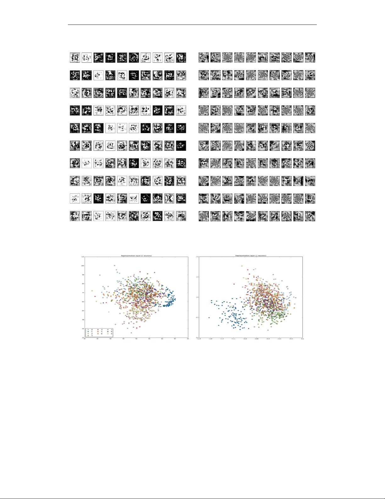
Under revie w as a conference paper at ICLR 2017 O P T I M A L B I N A RY A U T O E N C O D I N G W I T H P A I RW I S E C O R R E L A T I O N S Akshay Balsubramani ∗ abalsubr@ucsd.edu A B S T R A C T W e formulate learning of a binary autoencoder as a bicon vex optimization problem which learns from the pairwise correlations between encoded and decoded bits. Among all possible algorithms that use this information, ours finds the autoencoder that reconstructs its inputs with worst-case optimal loss. The optimal decoder is a single layer of artificial neurons, emerging entirely from the minimax loss minimization, and with weights learned by con vex optimization. All this is reflected in competiti ve experimental results, demonstrating that binary autoencoding can be done efficiently by con veying information in pairwise correlations in an optimal fashion. 1 I N T R O D U C T I O N Consider a general autoencoding scenario, in which an algorithm learns a compression scheme for independently , identically distributed (i.i.d.) V -dimensional bit vector data  x (1) , . . . , x ( n )  . For some encoding dimension H , the algorithm encodes each data example x ( i ) = ( x ( i ) 1 , . . . , x ( i ) V ) > into an H -dimensional representation e ( i ) , with H < V . It then decodes each e ( i ) back into a reconstructed example ˜ x ( i ) using some small amount of additional memory , and is evaluated on the quality of the reconstruction by the cross-entropy loss commonly used to compare bit vectors. A good autoencoder learns to compress the data into H bits so as to reconstruct it with low loss. When the loss is squared reconstruction error and the goal is to compress data in R V to R H , this is often accomplished with principal component analysis (PCA), which projects the input data on the top H eigen vectors of their co variance matrix (Bourlard & Kamp (1988); Baldi & Hornik (1989)). These eigen vectors in R V constitute V H real v alues of additional memory needed to decode the compressed data in R H back to the reconstructions in R V , which are linear combinations of the eigen vectors. Crucially , this total additional memory does not depend on the amount of data n , making it applicable when data are abundant. This paper considers a similar problem, e xcept using bit-vector data and the cross-entropy recon- struction loss. Since we are compressing samples of i.i.d. V -bit data into H -bit encodings, a natural approach is to remember the pairwise statistics: the V H av erage correlations between pairs of bits in the encoding and decoding, constituting as much additional memory as the eigenv ectors used in PCA. The decoder uses these along with the H -bit encoded data, to produce V -bit reconstructions. W e show how to ef ficiently learn the autoencoder with the worst-case optimal loss in this scenario, without any further assumptions, parametric or otherwise. It has some striking properties. The decoding function is identical in form to the one used in a standard binary autoencoder with one hidden layer (Bengio et al. (2013a)) and cross-entropy reconstruction loss. Specifically , each bit v of the decoding is the output of a logistic sigmoid artificial neuron of the encoded bits, with some learned weights w v ∈ R H . This form emerges as the uniquely optimal decoding function, and is not assumed as part of any e xplicit model. The worst-case optimal reconstruction loss suf fered by the autoencoder is con vex in these decoding weights W = { w v } v ∈ [ V ] , and in the encoded representations E . Though it is not jointly conv ex ∗ Most of the work was done as a PhD student at UC San Die go. Now reachable at: abalsubr@stanford.edu . 1 Under revie w as a conference paper at ICLR 2017 in both, the situation still admits a natural and efficient optimization algorithm in which the loss is alternately minimized in E and W while the other is held fixed. The algorithm is practical, learning incrementally from minibatches of data in a stochastic optimization setting. 1 . 1 N O T AT I O N The decoded and encoded data can be written in matrix form, representing bits as ± 1 : X =    x (1) 1 · · · x ( n ) 1 . . . . . . . . . x (1) V · · · x ( n ) V    ∈ [ − 1 , 1] V × n , E =    e (1) 1 · · · e ( n ) 1 . . . . . . . . . e (1) H · · · e ( n ) H    ∈ [ − 1 , 1] H × n (1) Here the encodings are allowed to be randomized, represented by v alues in [ − 1 , 1] instead of just the two v alues {− 1 , 1 } ; e.g. e (1) i = 1 2 is +1 w .p. 3 4 and − 1 w .p. 1 4 . The data in X are also allowed to be randomized, which loses hardly an y generality for reasons discussed later (Appendix B). W e write the columns of X , E as x ( i ) , e ( i ) for i ∈ [ n ] (where [ s ] := { 1 , . . . , s } ), representing the data. The rows are written as x v = ( x (1) v , . . . , x ( n ) v ) > for v ∈ [ V ] and e h = ( e (1) h , . . . , e ( n ) h ) > for h ∈ [ H ] . W e also consider the correlation of each bit h of the encoding with each decoded bit v ov er the data, i.e. b v ,h := 1 n P n i =1 x ( i ) v e ( i ) h . This too can be written in matrix form as B := 1 n XE > ∈ R V × H , whose rows and columns we respecti vely write as b v = ( b v , 1 , . . . , b v ,H ) > ov er v ∈ [ V ] and b h = ( b 1 ,h , . . . , b V ,h ) > ov er h ∈ [ H ] ; the indexing will be clear from conte xt. As alluded to earlier , the loss incurred on example i ∈ [ n ] is the cross-entropy between the example x ( i ) and its reconstruction ˜ x ( i ) , in expectation over the randomness in x ( i ) . Defining ` ± ( ˜ x ( i ) v ) = ln  2 1 ± ˜ x ( i ) v  (the partial losses to true labels ± 1 ), the loss is written as: ` ( x ( i ) , ˜ x ( i ) ) := V X v =1 " 1 + x ( i ) v 2 ! ` + ( ˜ x ( i ) v ) + 1 − x ( i ) v 2 ! ` − ( ˜ x ( i ) v ) # (2) In addition, define a potential well Ψ( m ) := ln (1 + e m ) + ln (1 + e − m ) with deriv ativ e Ψ 0 ( m ) := 1 − e − m 1+ e − m . Univ ariate functions like this are applied componentwise to matrices in this paper . 1 . 2 P R O B L E M S E T U P W ith these definitions, the autoencoding problem we address can be precisely stated as two tasks, encoding and decoding. These share only the side information B . Our goal is to perform these steps so as to achiev e the best possible guarantee on reconstruction loss, with no further assumptions. This can be written as a zero-sum game of an autoencoding algorithm seeking to minimize loss against an adversary , by playing encodings and reconstructions: • Using X , algorithm plays (randomized) encodings E , resulting in pairwise correlations B . • Using E and B , algorithm plays reconstructions ˜ X =  ˜ x (1) ; . . . ; ˜ x ( n )  ∈ [ − 1 , 1] V × n . • Giv en ˜ X , E , B , adversary plays X to maximize reconstruction loss 1 n P n i =1 ` ( x ( i ) , ˜ x ( i ) ) . W e find the autoencoding algorithm’ s best strategy in two parts. First, we find the optimal decoding of any encodings E giv en B , in Section 2. Then, we use the resulting optimal reconstruction function to outline the best encoding procedure, i.e. one that finds the E , B that lead to the best reconstruction, in Section 3.1. Combining these ideas yields an autoencoding algorithm in Section 3.2 (Algorithm 1), where its implementation and interpretation are specified. Further discussion and related work in Section 4 are followed by more e xtensions in Section 5 and experiments in Section 6. 2 O P T I M A L L Y D E C O D I N G A N E N C O D E D R E P R E S E N T A T I O N T o address the problem of Section 1.2, we first assume E and B are fixed, and deri ve the optimal decoding rule giv en this information. W e show in this section that the form of this optimal decoder is 2 Under revie w as a conference paper at ICLR 2017 precisely the same as in a classical autoencoder: having learned a weight vector w v ∈ R H for each v ∈ [ V ] , the v th bit of each reconstruction ˜ x i is expressed as a logistic function of a w v -weighted combination of the H encoded bits e i – a logistic artificial neuron with weights w v . The weight vectors are learned by con ve x optimization, despite the nonconv exity of the transfer functions. T o de velop this, we minimize the worst-case reconstruction error , where X is constrained by our prior knowledge that B = 1 n XE > , i.e. 1 n Ex v = b v ∀ v ∈ [ V ] . This can be written as a function of E : L ∗ B ( E ) := min ˜ x (1) ,..., ˜ x ( n ) ∈ [ − 1 , 1] V max x (1) ,..., x ( n ) ∈ [ − 1 , 1] V , ∀ v ∈ [ V ]: 1 n Ex v = b v 1 n n X i =1 ` ( x ( i ) , ˜ x ( i ) ) (3) W e solve this minimax problem for the optimal reconstructions played by the minimizing player in (3), written as ˜ x (1) ∗ , . . . , ˜ x ( n ) ∗ . Theorem 1. Define the bitwise slack function γ E ( w , b ) := − b > w + 1 n P n i =1 Ψ( w > e ( i ) ) , which is con vex in w . W .r .t. any b v , this has minimizing weights w ∗ v := w ∗ v ( E , B ) := arg min w ∈ R H γ E ( w , b v ) . Then the minimax value of the game (3) is L ∗ B ( E ) = 1 2 V X v =1 γ E ( w ∗ v , b v ) . F or any example i ∈ [ n ] , the minimax optimal r econstruction can be written for any bit v as ˜ x ( i ) ∗ v := 1 − e − w ∗> v e ( i ) 1+ e − w ∗> v e ( i ) . This tells us that the optimization problem of finding the minimax optimal reconstructions ˜ x ( i ) is extremely con venient in sev eral respects. The learning problem decomposes over the V bits in the decoding, reducing to solving for a weight vector w ∗ v ∈ R H for each bit v , by optimizing each bitwise slack function. Gi ven the weights, the optimal reconstruction of any example i can be specified by a layer of logistic sigmoid artificial neurons of its encoded bits, with w ∗> v e ( i ) as the bitwise logits. Hereafter , we write W ∈ R V × H as the matrix of decoding weights, with ro ws { w v } V v =1 . In particular , the optimal decoding weights W ∗ ( E , B ) are the matrix with ro ws { w ∗ v ( E , B ) } V v =1 . 3 L E A R N I N G A N A U T O E N C O D E R 3 . 1 F I N D I N G A N E N C O D E D R E P R E S E N T AT I O N Having computed the optimal decoding function in the previous section given any E and B , we now switch perspectiv es to the encoder , which seeks to compress the input data X into encoded representations E (from which B is easily calculated to pass to the decoder). W e seek to find ( E , B ) to ensure the lowest worst-case reconstruction loss after decoding; recall that this is L ∗ B ( E ) from (3) . Observe that 1 n XE > = B , and that the encoder is giv en X . Therefore, in terms of X , L ∗ B ( E ) = 1 2 n n X i =1 V X v =1 h − x ( i ) v ( w ∗> v e ( i ) ) + Ψ( w ∗> v e ( i ) ) i := L ( W ∗ , E ) (4) by using Thm. 1 and substituting b v = 1 n Ex v ∀ v ∈ [ V ] . So it is conv enient to define the bitwise featur e distortion 1 for any v ∈ [ V ] with respect to W , between any e xample x and its encoding e : β W v ( e , x ) := − x v w > v e + Ψ( w > v e ) (5) From the above discussion, the best E giv en any decoding W , written as E ∗ ( W ) , solv es the minimization min E ∈ [ − 1 , 1] H × n L ( W , E ) = 1 2 n n X i =1 min e ( i ) ∈ [ − 1 , 1] H V X v =1 β W v ( e ( i ) , x ( i ) ) which immediately yields the following result. 1 Noting that Ψ( w > v e ) ≈   w > v e   , we see that β W v ( e , x ) ≈ w > v e  sgn( w > v e ) − x v  , so w > v e is encouraged to match signs with x v , motiv ating the name. 3 Under revie w as a conference paper at ICLR 2017 Proposition 2. Define the optimal encodings for decoding weights W as E ∗ ( W ) := arg min E ∈ [ − 1 , 1] H × n L ( W , E ) . Each example x ( i ) ∈ [ − 1 , 1] V can be separately encoded as e ( i ) ∗ ( W ) , with its optimal encoding minimizing its total featur e distortion over the decoded bits w .r .t. W : E N C ( x ( i ) ; W ) := e ( i ) ∗ ( W ) := arg min e ∈ [ − 1 , 1] H V X v =1 β W v ( e , x ( i ) ) (6) Observe that the encoding function E N C ( x ( i ) ; W ) can be ef ficiently computed to desired precision since the feature distortion β W v ( e , x ( i ) ) of each bit v is con vex and Lipschitz in e ; an L 1 error of  can be reached in O (  − 2 ) linear-time first-order optimization iterations. Note that the encodings need not be bits, and can be e.g. unconstrained ∈ R H instead; the proof of Thm. 1 assumes no structure on them. 3 . 2 A N A U TO E N C O D E R L E A R N I N G A L G O R I T H M Our ultimate goal is to minimize the worst-case reconstruction loss. As we hav e seen in (3) and (6) , it is con vex in the encoding E and in the decoding parameters W , each of which can be fixed while minimizing with respect to the other . This suggests a learning algorithm that alternately performs tw o steps: finding encodings E that minimize L ( W , E ) as in (6) with a fixed W , and finding decoding parameters W ∗ ( E , B ) , as given in Algorithm 1. Algorithm 1 Pairwise Correlation Autoencoder (P C - A E ) Input: Size- n dataset U Initialize W 0 (e.g. with each element being i.i.d. ∼ N (0 , 1) ) for t = 1 to T do Encode each example to ensure accurate reconstruction using weights W t − 1 , and compute the associated pairwise bit correlations B t : ∀ i ∈ [ n ] : [ e ( i ) ] t = E N C ( x ( i ) ; W t − 1 ) , B t = 1 n XE > t Update weight vectors [ w v ] t for each v ∈ [ V ] to minimize slack function, using encodings E t : ∀ v ∈ [ V ] : [ w v ] t = arg min w ∈ R H " − [ b v ] > t w + 1 n n X i =1 Ψ( w > e ( i ) t ) # end for Output: W eights W T 3 . 3 E FFI C I E N T I M P L E M E N T A T I O N Our deri vation of the encoding and decoding functions in volv es no model assumptions at all, only using the minimax structure and pairwise statistics that the algorithm is allowed to remember . Nev ertheless, the (en/de)coders can still be learned and implemented efficiently . Decoding is a con vex optimization in H dimensions, which can be done in parallel for each bit v ∈ [ V ] . This is relati vely easy to solve in the parameter re gime of primary interest when data are abundant, in which H < V  n . Similarly , encoding is also a con vex optimization problem in only H dimensions. If the data examples are instead sampled in minibatches of size n , they can be encoded in parallel, with a new minibatch being sampled to start each epoch t . The number of examples n (per batch) is essentially only limited by nH , the number of compressed representations that fit in memory . So far in this paper , we have stated our results in the transducti ve setting, in which all data are giv en together a priori, with no assumptions whatsoe ver made about the interdependences between the V features. Howe ver , P C - A E operates much more ef ficiently than this might suggest. Crucially , 4 Under revie w as a conference paper at ICLR 2017 the encoding and decoding tasks both depend on n only to average a function of x ( i ) or e ( i ) ov er i ∈ [ n ] , so they can both be solved by stochastic optimization methods that use first-order gradient information, like variants of stochastic gradient descent (SGD). W e find it remarkable that the minimax optimal encoding and decoding can be ef ficiently learned by such methods, which do not scale computationally in n . Note that the result of each of these steps in volv es Ω( n ) outputs ( E and ˜ X ), which are all coupled together in complex ways. The efficient implementation of first-order methods turns out to manipulate more intermediate gradient-related quantities with facile interpretations. For details, see Appendix A.2. 3 . 4 C O N V E R G E N C E A N D W E I G H T R E G U L A R I Z A T I O N As we noted previously , the objectiv e function of the optimization is bicon vex . This means that under broad conditions, the alternating minimization algorithm we specify is an instance of alternating con vex sear ch , sho wn in that literature to con verge under broad conditions (Gorski et al. (2007)). It is not guaranteed to con verge to the global optimum, but each iteration will monotonically decrease the objecti ve function. In light of our introductory discussion, the properties and rate of such con vergence would be interesting to compare to stochastic optimization algorithms for PCA, which con verge efficiently under broad conditions (Balsubramani et al. (2013); Shamir (2016)). The basic game used so f ar has assumed perfect knowledge of the pairwise correlations, leading to equality constraints ∀ v ∈ [ V ] : 1 n Ex v = b v . This makes sense in P C - A E , where the encoding phase of each epoch giv es the e xact B t for the decoding phase. Ho wever , in other stochastic settings as for denoising autoencoders (see Sec. 5.2), it may be necessary to relax this constraint. A relaxed constraint of   1 n Ex v − b v   ∞ ≤  exactly corresponds to an extra additi ve regularization term of  k w v k 1 on the corresponding weights in the con vex optimization used to find W (Appendix C.1). Such regularization leads to pro vably better generalization (Bartlett (1998)) and is often practical to use, e.g. to encourage sparsity . But we do not use it for our P C - A E experiments in this paper . 4 D I S C U S S I O N A N D R E L AT E D W O R K Our approach P C - A E is quite different from e xisting autoencoding work in sev eral ways. First and foremost, we posit no explicit decision rule, and av oid optimizing the highly non-con vex decision surface tra versed by traditional autoencoding algorithms that learn with backpropagation. The decoding function, gi ven the encodings, is a single layer of artificial neurons only because of the minimax structure of the problem when minimizing worst-case loss. This differs from reasoning typically used in neural net work (see Jordan (1995)), in which the loss is the ne gative log-lik elihood (NLL) of the joint probability , which is assumed to follow a form specified by logistic artificial neurons and their weights. W e instead interpret the loss in the usual direct way as the NLL of the predicted probability of the data gi ven the visible bits, and a void an y assumptions on the decision rule (e.g. not monotonicity in the score w > v e ( i ) , or e ven dependence on such a score). This justification of artificial neurons – as the minimax optimal decision rules given information on pairwise correlations – is one of our more distinctiv e contributions (see Sec. 5.1). Note that there are no assumptions whatsoe ver on the form of the encoding or decoding, except on the memory used by the decoding. Some such restriction is necessary to rule out the autoencoder just memorizing the data, and is typically expressed by positing a model class of compositions of artificial neuron layers. W e instead impose it axiomiatically by limiting the amount of information transmitted through B , which does not scale in n ; but we do not restrict how this information is used. This confers a clear theoretical adv antage, allowing us to attain the strongest robust loss guarantee among all possible autoencoders that use the correlations B . More importantly in practice, avoiding an e xplicit model class means that we do not have to optimize the typically non-con vex model, which has long been a central issue for backpropagation-based learning methods (e.g. Dauphin et al. (2014)). Prior work related in spirit has attempted to a void this through con vex relaxations, including for multi-layer optimization under v arious structural assumptions (Aslan et al. (2014); Zhang et al. (2016)), and when the number of hidden units is v aried by the algorithm (Bengio et al. (2005); Bach (2014)). 5 Under revie w as a conference paper at ICLR 2017 Our approach also isolates the benefit of higher n in dealing with ov erfitting, as the pairwise correlations B can be measured progressively more accurately as n increases. In this respect, we follow a line of research using such pairwise correlations to model arbitary higher-order structure among visible units, rooted in early work on (restricted) Boltzmann Machines (Ackley et al. (1985); Smolensky (1986); Rumelhart & McClelland (1987); Freund & Haussler (1992)). More recently , theoretical algorithms have been developed with the perspectiv e of learning from the correlations between units in a network, under v arious assumptions on the activ ation function, architecture, and weights, for both deep (Arora et al. (2014)) and shallo w networks (using tensor decompositions, e.g. Livni et al. (2014); Janzamin et al. (2015)). Our use of ensemble aggregation techniques (from Balsubramani & Freund (2015a; 2016)) to study these problems is anticipated in spirit by prior work as well, as discussed at length by Bengio (2009) in the context of distrib uted representations. 4 . 1 O P T I M A L I T Y , O T H E R A R C H I T E C T U R E S A N D D E P T H W e have established that a single layer of logistic artificial neurons is an optimal decoder, given only indirect information about the data through pairwise correlations. This is not a claim that autoencoders need only a single-layer architecture in the worst case. Sec. 3.1 establishes that the best representations E are the solution to a conv ex optimization, with no artificial neurons in volved in computing them from the data. Unlike the decoding function, the optimal encoding function E N C cannot be written explicitly in terms of artificial neurons, and is incomparable to existing architectures. Also, the encodings are only optimal giv en the pairwise correlations; training algorithms like backpropagation, which indirectly communicate other kno wledge of the input data through deriv ativ e composition, can certainly learn final decoding layers that outperform ours, as we see in experiments. In our frame work so far , we explore using all the pairwise correlations between hidden and visible bits to inform learning by constraining the adversary , resulting in a Lagrange parameter – a weight – for each constraint. These V H weights W constitute the parameters of the optimal decoding layer , describing a fully connected architecture. If just a select fe w of these correlations were used, only they would constrain the adversary in the minimax problem of Sec. 2, so weights would only be introduced for them, giving rise to sparser architectures. Our central choices to store only pairwise correlations and minimize w orst-case reconstruction loss play a similar regularizing role to e xplicit model assumptions, and other autoencoding methods may achiev e better performance on data for which these choices are too conserv ative, by e.g. making distributional assumptions on the data. From our perspecti ve, other architectures with more layers – particularly highly successful ones like con volutional, recurrent, residual, and ladder networks (LeCun et al. (2015); He et al. (2015); Rasmus et al. (2015)) – lend the autoencoding algorithm more power by allo wing it to measure more nuanced correlations using more parameters, which decreases the worst-case loss. Applying our approach with these would be interesting future work. Extending this paper’ s conv enient minimax characterization to deep representations with empirical success is a very interesting open problem. Prior work on stacking autoencoders/RBMs (V incent et al. (2010)) and our learning algorithm P C - A E suggest that we could train a deep network in alternating forward and backward passes. Using this paper’ s ideas, the forward pass would learn the weights to each layer gi ven the previous layer’ s activ ations (and inter-layer pairwise correlations) by minimizing the slack function, with the backward pass learning the acti vations for each layer gi ven the weights to / acti vations of the next layer by conv ex optimization (as we learn E ). Both passes consist of successi ve con vex optimizations dictated by our approach, quite distinct from backpropagation, though they loosely resemble the wake-sleep algorithm (Hinton et al. (1995)). 4 . 2 G E N E R A T I V E A P P L I C A T I O N S Particularly recently , autoencoders hav e been of interest largely for their man y applications beyond compression, especially for their generative uses. The most directly rele vant to us in volv e repurposing denoising autoencoders (Bengio et al. (2013b); see Sec. 5.2); moment matching among hidden and visible units (Li et al. (2015)); and generativ e adversarial network ideas (Goodfello w et al. (2014); Makhzani et al. (2015)), the latter particularly since the techniques of this paper hav e been applied to binary classification (Balsubramani & Freund (2015a;b)). These are outside this paper’ s scope, but suggest themselves as future e xtensions of our approach. 6 Under revie w as a conference paper at ICLR 2017 5 E X T E N S I O N S 5 . 1 O T H E R R E C O N S T RU C T I O N L O S S E S It may make sense to use another reconstruction loss other than cross-entropy , for instance the expected Hamming distance between x ( i ) and ˜ x ( i ) . It turns out that the minimax manipulations we use work under very broad conditions, for nearly any loss that additi vely decomposes over the V bits as cross-entrop y does. In such cases, all that is required is that the partial losses ` + ( ˜ x ( i ) v ) , ` − ( ˜ x ( i ) v ) are monotonically decreasing and increasing respecti vely (recall that for cross-entrop y loss, this is true as ` ± ( ˜ x ( i ) v ) = ln  2 1 ± ˜ x ( i ) v  ); they need not e ven be con vex. This monotonicity is a natural condition, because the loss measures the discrepancy to the true label, and holds for all losses in common use. Changing the partial losses only changes the structure of the minimax solution in two respects: by altering the form of the transfer function on the decoding neurons, and the univ ariate potential well Ψ optimized to learn the decoding weights. Otherwise, the problem remains conv ex and the algorithm is identical. Formal statements of these general results are in Appendix D. 5 . 2 D E N O I S I N G A U T O E N C O D I N G Our frame work can be easily applied to learn a denoising autoencoder (D AE; V incent et al. (2008; 2010)), which uses noise-corrupted data (call it ˆ X ) for training, and uncorrupted data for ev aluation. From our perspectiv e, this corresponds to leaving the learning of W unchanged, but using corrupted data when learning E . So the minimization problem over encodings must be changed to account for the bias on B introduced by the noise, so that the algorithm plays giv en the noisy data, but to minimize loss against X . This is easiest to see for zero-mean noise, for which our algorithms are completely unchanged because B does not change after adding noise. Another common scenario illustrating this technique is to mask a ρ fraction of the input bits uniformly at random (in our notation, changing 1 s to − 1 s). This masking noise changes each pairwise correlation b v ,h by an amount δ v ,h := 1 n P n i =1 ( ˆ x ( i ) v − x ( i ) v ) e ( i ) h , so the optimand Eq. (4) must therefore be modified by subtracting this factor . δ v ,h can be estimated (w .h.p.) given ˆ x v , e h , ρ, x v . But e ven with just the noisy data and not x v , we can estimate δ v ,h w .h.p. by extrapolating the correlation of the bits of ˆ x v that are left as +1 (a 1 − ρ fraction) with the corresponding values in e h . 6 E X P E R I M E N T S In this section we compare our approach empirically to standard autoencoders with one hidden layer (termed AE here) trained with backpropagation. Our goal is simply to v erify that our very distinct approach is competitiv e in reconstruction performance with cross-entropy loss. The datasets we use are first normalized to [0 , 1] , and then binarized by sampling each pixel stochasti- cally in proportion to its intensity , following prior work (Salakhutdinov & Murray (2008)). Choosing between binary and real-v alued encodings in P C - A E requires just a line of code, to project the en- codings into [ − 1 , 1] V after con vex optimization updates to compute E N C ( · ) . W e use Adagrad (Duchi et al. (2011)) for the con vex minimizations of our algorithms; we observ ed that their performance is not very sensiti ve to the choice of optimization method, explained by our approach’ s con vexity . W e compare to a basic single-layer AE trained with the Adam method with default parameters in Kingma & Ba (2014). Other models lik e variational autoencoders (Kingma & W elling (2013)) are not shown here because they do not aim to optimize reconstruction loss or are not comparably general autoencoding architectures (see Appendix A). W e try 32 and 100 hidden units for both algorithms, and try both binary and unconstrained real-valued encodings; the respecti ve AE uses logistic and ReLU transfer functions for the encoding neurons. The results are in T able 1. The reconstruction performance of P C - A E indicates that it can encode information very well using pairwise correlations. Loss can become extremely lo w when H is raised, gi ving B the capacity to encode far more information. The performance is marginally better with binary hidden units than unconstrained ones, in accordance with the spirit of our deriv ations. 7 Under revie w as a conference paper at ICLR 2017 T able 1: Cross-entropy reconstruction losses for P C - A E and a vanilla single-layer autoencoder , with binary and unconstrained real-valued encodings. P C - A E (bin.) P C - A E (real) AE (bin.) AE (real) MNIST , H = 32 51.9 53.8 65.2 64.3 MNIST , H = 100 9.2 9.9 26.8 25.0 Omniglot, H = 32 76.1 77.2 93.1 90.6 Omniglot, H = 100 12.1 13.2 46.6 45.4 Caltech-101, H = 32 54.5 54.9 97.5 87.6 Caltech-101, H = 100 7.1 7.1 64.3 45.4 notMNIST , H = 32 121.9 122.4 149.6 141.8 notMNIST , H = 100 62.2 63.0 99.6 92.1 W e also try learning just the decoding layer of Sec. 2, on the encoded representation of the AE. This is moti vated by the fact that establishes our decoding method to be w orst-case optimal given an y E and B . W e find the results to be significantly worse than the AE alone on all datasets (reconstruction loss of ∼ 171 / 133 on MNIST , and ∼ 211 / 134 on Omniglot, with 32 / 100 hidden units respectiv ely). This reflects the AE’ s backprop training propagating information about the data beyond pairwise correlations through non-con vex function compositions – ho wever , the cost of this is that they are more difficult to optimize. The representations learned by the E N C function of P C - A E are quite different and capture much more of the pairwise correlation information, which is used by the decoding layer in a w orst-case optimal fashion. W e attempt to visually depict the dif ferences between the representations in Fig. 3. Figure 1: T op row: random test images from Omniglot. Middle and bottom rows: reconstructions of P C - A E and AE with H = 100 binary hidden units. Difference in quality is particularly noticeable in the 1st, 5th, 8th, and 11th columns. Figure 2: As Fig. 1, with H = 32 on Caltech-101 silhouettes. As discussed in Sec. 4, we do not claim that our method will always achiev e the best empirical reconstruction loss, e ven among single-layer autoencoders. W e would like to make the encoding function quicker to compute, as well. But we believe this paper’ s results, especially when H is high, illustrate the potential of using pairwise correlations for autoencoding as in our approach, learning to encode with alternating con vex minimization and extremely strong worst-case rob ustness guarantees. 8 Under revie w as a conference paper at ICLR 2017 Figure 3: T op three rows: the reconstructions of random test images from MNIST ( H = 12 ), as in Fig. 1. P C - A E achiev es loss 105 . 1 here, and AE 111 . 2 . Fourth and fifth rows: visualizations of all the hidden units of P C - A E and AE, respectiv ely . It is not possible to visualize the P C - A E encoding units by the image that maximally activ ates them, as commonly done, because of the form of the E N C function which depends on W and lacks explicit encoding weights. So each hidden unit h is depicted by the visible decoding of the encoded representation which has bit h "on" and all other bits "of f." (If this were PCA with a linear decoding layer , this would simply represent hidden unit h by its corresponding principal component vector , the decoding of the h th canonical basis vector in R H .) A C K N OW L E D G M E N T S I am grateful to Jack Berko witz, Sanjoy Dasgupta, and Y oav Freund for helpful discussions; Daniel Hsu and Akshay Krishnamurthy for instructi ve examples; and Gary Cottrell for enjoyable chats. R E F E R E N C E S David H Ackle y , Geoffre y E Hinton, and T errence J Sejnowski. A learning algorithm for boltzmann machines. Cognitive science , 9(1):147–169, 1985. Sanjeev Arora, Aditya Bhaskara, Rong Ge, and T engyu Ma. Provable bounds for learning some deep representations. In Proceedings of the 31st International Confer ence on Machine Learning (ICML-14) , pp. 584–592, 2014. Özlem Aslan, Xinhua Zhang, and Dale Schuurmans. Con ve x deep learning via normalized kernels. In Advances in Neural Information Pr ocessing Systems , pp. 3275–3283, 2014. Francis Bach. Breaking the curse of dimensionality with conv ex neural networks. arXiv pr eprint arXiv:1412.8690 , 2014. Pierre Baldi. Autoencoders, unsupervised learning, and deep architectures. Unsupervised and T ransfer Learning Challeng es in Machine Learning, V olume 7 , pp. 43, 2012. Pierre Baldi and Kurt Hornik. Neural networks and principal component analysis: Learning from examples without local minima. Neural networks , 2(1):53–58, 1989. Akshay Balsubramani and Y oav Freund. Optimally combining classifiers using unlabeled data. In Confer ence on Learning Theory (COLT) , 2015a. Akshay Balsubramani and Y oav Freund. Scalable semi-supervised classifier aggreg ation. In Advances in Neural Information Pr ocessing Systems (NIPS) , 2015b. Akshay Balsubramani and Y oav Freund. Optimal binary classifier aggregation for general losses. In Advances in Neural Information Pr ocessing Systems (NIPS) , 2016. Akshay Balsubramani, Sanjoy Dasgupta, and Y oav Freund. The fast con ver gence of incremental pca. In Advances in Neural Information Pr ocessing Systems (NIPS) , pp. 3174–3182, 2013. 9 Under revie w as a conference paper at ICLR 2017 Peter L Bartlett. The sample complexity of pattern classification with neural networks: the size of the weights is more important than the size of the network. IEEE T ransactions on Information Theory , 44(2):525–536, 1998. Y oshua Bengio. Learning deep architectures for ai. F oundations and T rends in Mac hine Learning , 2 (1):1–127, 2009. Y oshua Bengio, Nicolas L Roux, P ascal V incent, Olivier Delalleau, and Patrice Marcotte. Conv ex neural networks. In Advances in neural information processing systems (NIPS) , pp. 123–130, 2005. Y oshua Bengio, Aaron Courville, and Pierre V incent. Representation learning: A revie w and new perspecti ves. P attern Analysis and Machine Intelligence, IEEE T ransactions on , 35(8):1798–1828, 2013a. Y oshua Bengio, Li Y ao, Guillaume Alain, and Pascal V incent. Generalized denoising auto-encoders as generati ve models. In Advances in Neur al Information Pr ocessing Systems (NIPS) , pp. 899–907, 2013b. Hervé Bourlard and Yves Kamp. Auto-association by multilayer perceptrons and singular v alue decomposition. Biological cybernetics , 59(4-5):291–294, 1988. Y uri Burda, Roger Grosse, and Ruslan Salakhutdinov . Importance weighted autoencoders. Interna- tional Confer ence on Learning Representations (ICLR) , 2016. arXiv preprint arXi v:1509.00519. Nicolo Cesa-Bianchi and Gàbor Lugosi. Prediction, Learning , and Games . Cambridge Uni versity Press, New Y ork, NY , USA, 2006. Y ann N Dauphin, Razvan P ascanu, Caglar Gulcehre, Kyunghyun Cho, Surya Ganguli, and Y oshua Bengio. Identifying and attacking the saddle point problem in high-dimensional non-conv ex optimization. In Advances in neural information pr ocessing systems (NIPS) , pp. 2933–2941, 2014. John Duchi, Elad Hazan, and Y oram Singer . Adapti ve subgradient methods for online learning and stochastic optimization. The J ournal of Machine Learning Resear ch , 12:2121–2159, 2011. Y oav Freund and David Haussler . Unsupervised learning of distributions on binary vectors using two layer networks. In Advances in Neural Information Pr ocessing Systems (NIPS) , pp. 912–919, 1992. Ian Goodfellow , Jean Pouget-Abadie, Mehdi Mirza, Bing Xu, David W arde-Farley , Sherjil Ozair, Aaron Courville, and Y oshua Bengio. Generativ e adv ersarial nets. In Advances in Neur al Information Pr ocessing Systems (NIPS) , pp. 2672–2680, 2014. Jochen Gorski, Frank Pfeuffer , and Kathrin Klamroth. Bicon vex sets and optimization with bicon vex functions: a survey and extensions. Mathematical Methods of Oper ations Resear ch , 66(3):373–407, 2007. Kaiming He, Xiangyu Zhang, Shaoqing Ren, and Jian Sun. Deep residual learning for image recognition. arXiv pr eprint arXiv:1512.03385 , 2015. Geoffre y E Hinton, Peter Dayan, Brendan J Frey , and Radford M Neal. The" wake-sleep" algorithm for unsupervised neural networks. Science , 268(5214):1158–1161, 1995. Majid Janzamin, Hanie Sedghi, and Anima Anandkumar . Beating the perils of non-con ve xity: Guaranteed training of neural networks using tensor methods. arXiv pr eprint arXiv:1506.08473 , 2015. Michael I Jordan. Why the logistic function? a tutorial discussion on probabilities and neural networks, 1995. Diederik Kingma and Jimmy Ba. Adam: A method for stochastic optimization. arXiv pr eprint arXiv:1412.6980 , 2014. Diederik P Kingma and Max W elling. Auto-encoding v ariational bayes. arXiv pr eprint arXiv:1312.6114 , 2013. 10 Under revie w as a conference paper at ICLR 2017 Y ann LeCun, Y oshua Bengio, and Geoffre y Hinton. Deep learning. Natur e , 521(7553):436–444, 2015. Y ujia Li, Ke vin Swersky , and Rich Zemel. Generative moment matching netw orks. In Pr oceedings of the 32nd International Confer ence on Machine Learning (ICML-15) , pp. 1718–1727, 2015. Roi Li vni, Shai Shale v-Shwartz, and Ohad Shamir . On the computational ef ficiency of training neural networks. In Advances in Neural Information Pr ocessing Systems (NIPS) , pp. 855–863, 2014. Alireza Makhzani, Jonathon Shlens, Navdeep Jaitly , and Ian Goodfello w . Adv ersarial autoencoders. arXiv pr eprint arXiv:1511.05644 , 2015. Antti Rasmus, Mathias Ber glund, Mikko Honkala, Harri V alpola, and T apani Raiko. Semi-supervised learning with ladder networks. In Advances in Neural Information Pr ocessing Systems , pp. 3546– 3554, 2015. David E Rumelhart and James L McClelland. Parallel distributed processing, explorations in the microstructure of cognition. vol. 1: Foundations. Computational Models of Cognition and P er ception, Cambridge: MIT Pr ess , 1987. Ruslan Salakhutdinov and Iain Murray . On the quantitativ e analysis of deep belief networks. In Pr oceedings of the 25th International Conference on Machine Learning (ICML) , pp. 872–879, 2008. Ohad Shamir . Con vergence of stochastic gradient descent for pca. International Confer ence on Machine Learning (ICML) , 2016. arXiv preprint arXi v:1509.09002. P Smolensky . Information processing in dynamical systems: foundations of harmony theory . In P arallel distributed pr ocessing: e xplorations in the micr ostructure of cognition, vol. 1 , pp. 194–281. MIT Press, 1986. Pascal V incent, Hugo Larochelle, Y oshua Bengio, and Pierre-Antoine Manzagol. Extracting and composing robust features with denoising autoencoders. In Pr oceedings of the 25th international confer ence on Machine learning (ICML) , pp. 1096–1103. A CM, 2008. Pascal V incent, Hugo Larochelle, Isabelle Lajoie, Y oshua Bengio, and Pierre-Antoine Manzagol. Stacked denoising autoencoders: Learning useful representations in a deep network with a local denoising criterion. The J ournal of Machine Learning Resear ch , 11:3371–3408, 2010. Y uchen Zhang, Percy Liang, and Martin J W ainwright. Con vexified con volutional neural networks. arXiv pr eprint arXiv:1609.01000 , 2016. 11 Under revie w as a conference paper at ICLR 2017 A E X P E R I M E N T A L D E TA I L S In addition to MNIST , we used the preprocessed version of the Omniglot dataset in Burda et al. (2016), split 1 of the Caltech-101 Silhouettes dataset, and the small notMNIST dataset. Only notMNIST comes without a predefined split, so the displayed results use 10-fold cross-validation. Non-binarized versions of all datasets resulted in nearly identical P C - A E performance (not shown), as would be expected from its deri vation using e xpected pairwise correlations. W e used minibatches of size 250. All autoencoders were initialized with the ’Xavier’ initialization and trained for 500 epochs or using early stopping on the test set. W e did not ev aluate against other types of autoencoders which regularize (Kingma & W elling (2013)) or are otherwise not trained for direct reconstruction loss minimization. Also, not sho wn is the performance of a standard con volutional autoencoder (32-bit representation, depth-3 64-64-32 (en/de)coder) which is some what better than the standard autoencoder , but is still outperformed by P C - A E on our datasets. A deeper architecture could quite possibly achie ve superior performance, but the greater number of channels through which information is propagated mak es fair comparison with our flat fully-connected approach dif ficult. W e consider e xtension of our P C - A E approach to such architectures to be fascinating future work. A . 1 F U R T H E R R E S U L T S Our bound on worst-case loss is in variably quite tight, as shown in Fig. 4. Similar results are found on all datasets. This is consistent with our conclusions about the nature of the P C - A E representations – con veying almost e xactly the information av ailable in pairwise correlations. Figure 4: Actual reconstruction loss to real data (red) and slack function [objectiv e function] value (dotted green), during an Adagrad optimization to learn W using the optimal E , B . Monotonicity is expected since this is a con vex optimization. The objective function v alue theoretically upper-bounds the actual loss, and practically tracks it nearly perfectly . A 2D visualization of MNIST in Fig. 6, showing that e ven with just two hidden units there is enough information in pairwise correlations for P C - A E to learn a sensible embedding. W e also include more pictures of our autoencoders’ reconstructions, and visualizations of the hidden units when H = 100 in Fig. 5. A . 2 P C - A E I N T E R P R E TA T I O N A N D I M P L E M E N TA T I O N D E T A I L S Here we gi ve some details that are useful for interpretation and implementation of the proposed method. 12 Under revie w as a conference paper at ICLR 2017 Figure 5: V isualizations of all the hidden units of PC-AE (left) and AE (right) from Omniglot for H = 100 , as in Fig. 3. Figure 6: AE (left) and P C - A E (right) visualizations of a random subset of MNIST test data, with H = 2 real-valued hidden units, and colors corresponding to class labels (le gend at left). P C - A E ’ s loss is ∼ 189 here, and that of AE is ∼ 179 . A . 2 . 1 E N C O D I N G Proposition 2 defines the encoding function for any data e xample x as the vector that minimizes the total feature distortion, summed ov er the bits in the decoding, rewritten here for con venience: E N C ( x ( i ) ; W ) := arg min e ∈ [ − 1 , 1] H V X v =1 h − x ( i ) v w > v e ( i ) + Ψ( w > v e ( i ) ) i (7) Doing this on multiple examples at once (in memory as a minibatch) can be much faster than on each example separately . W e can now compute the gradient of the objective function w .r .t. each 13 Under revie w as a conference paper at ICLR 2017 Figure 7: As Fig. 1, with H = 100 on Caltech-101 silhouettes. Figure 8: As Fig. 1, with H = 100 on MNIST . example i ∈ [ n ] , writing the gradient w .r .t. example i as column i of a matrix G ∈ R H × n . G can be calculated efficiently in a number of w ays, for example as follows: • Compute matrix of hallucinated data ˘ X := Ψ 0 ( WE ) ∈ R V × n . • Subtract X to compute residuals R := ˘ X − X ∈ R V × n . • Compute G = 1 n W > R ∈ R H × n . Optimization then proceeds with gradient descent using G , with the step size found using line search. Note that since the objectiv e function is con vex, the optimum E ∗ leads to optimal residuals R ∗ ∈ R V × n such that G = 1 n W > R ∗ = 0 H × n , so each column of R ∗ is in the null space of W > , which maps the residual vectors to the encoded space. W e conclude that although the compression is not perfect (so the optimal residuals R ∗ 6 = 0 V × n in general), each column of R ∗ is orthogonal to the decoding weights at an equilibrium towards which the conv ex minimization problem of (7) is guaranteed to stably con verge. A . 2 . 2 D E C O D I N G The decoding step finds W to ensure accurate decoding of the giv en encodings E with correlations B , solving the con vex minimization problem: W ∗ = arg min W ∈ R V × H V X v =1 " − b > v w v + 1 n n X i =1 Ψ( w > v e ( i ) ) # (8) This can be minimized by first-order con vex optimization. The gradient of (8) at W is: − B + 1 n [Ψ 0 ( WE )] E > (9) The second term can be understood as “hallucinated" pairwise correlations ˘ B , between bits of the encoded examples E and bits of their decodings under the current weights, ˘ X := Ψ 0 ( WE ) . The hallucinated correlations can be written as ˘ B := 1 n ˘ XE > . Therefore, (9) can be interpreted as the residual correlations ˘ B − B . Since the slack function of (8) is conv ex, the optimum W ∗ leads to hallucinated correlations ˘ B ∗ = B , which is the limit reached by the optimization algorithm after many iterations. 14 Under revie w as a conference paper at ICLR 2017 Figure 9: As Fig. 1, with H = 32 on notMNIST . B A L L O W I N G R A N D O M I Z E D D A TA A N D E N C O D I N G S In this paper , we represent the bit-vector data in a randomized way in [ − 1 , 1] V . Randomizing the data only relaxes the constraints on the adv ersary in the game we play; so at worst we are working with an upper bound on worst-case loss, instead of the exact minimax loss itself, erring on the conservati ve side. Here we briefly justify the bound as being essentially tight, which we also see empirically in this paper’ s experiments. In the formulation of Section 2, the only information we have about the data is its pairwise correlations with the encoding units. When the data are abundant ( n large), then w .h.p. these correlations are close to their expected values o ver the data’ s internal randomization, so representing them as continuous values w .h.p. results in the same B and therefore the same solutions for E , W . W e are ef fectively allowing the adv ersary to play each bit’ s conditional probability of firing, rather than the binary realization of that probability . This allows us to apply minimax theory and duality to considerably simplify the problem to a conv ex optimization, when it would otherwise be noncon vex, and computationally hard (Baldi (2012)). The fact that we are only using information about the data through its expected pairwise correlations makes this possible. The abov e also applies to the encodings and their internal randomization, allowing us to learn binary randomized encodings by projecting to the con vex set [ − 1 , 1] H . C P R O O F S Pr oof of Theor em 1. Writing Γ( ˜ x ( i ) v ) := ` − ( ˜ x ( i ) v ) − ` + ( ˜ x ( i ) v ) = ln  1+ ˜ x ( i ) v 1 − ˜ x ( i ) v  for con venience, we can simplify L ∗ , using the definition of the loss (2) , and Lagrange duality for all V H constraints in volving B . This leads to the follo wing chain of equalities, where for bre vity the constraint sets are sometimes omitted when clear , and we write X as shorthand for the data x (1) , . . . , x ( n ) and ˜ X analogously for the reconstructions. L ∗ = 1 2 min ˜ x (1) ,..., ˜ x ( n ) ∈ [ − 1 , 1] V max x (1) ,..., x ( n ) ∈ [ − 1 , 1] V , ∀ v ∈ [ V ]: 1 n Ex v = b v 1 n n X i =1 V X v =1 h 1 + x ( i ) v  ` + ( ˜ x ( i ) v ) +  1 − x ( i ) v  ` − ( ˜ x ( i ) v ) i = 1 2 min ˜ X max X min W ∈ R V × H " 1 n n X i =1 V X v =1  ` + ( ˜ x ( i ) v ) + ` − ( ˜ x ( i ) v ) − x ( i ) v Γ( ˜ x ( i ) v )  + V X v =1 w > v  1 n Ex v − b v  # ( a ) = 1 2 min w 1 ,..., w V " − V X v =1 b > v w v + 1 n min ˜ X max X V X v =1 " n X i =1  ` + ( ˜ x ( i ) v ) + ` − ( ˜ x ( i ) v ) − x ( i ) v Γ( ˜ x ( i ) v )  + w > v Ex v ## = 1 2 min w 1 ,..., w V " − V X v =1 b > v w v + 1 n min ˜ X n X i =1 V X v =1  ` + ( ˜ x ( i ) v ) + ` − ( ˜ x ( i ) v ) + max x ( i ) ∈ [ − 1 , 1] V x ( i ) v  w > v e ( i ) − Γ( ˜ x ( i ) v )   # (10) 15 Under revie w as a conference paper at ICLR 2017 where ( a ) uses the minimax theorem (Cesa-Bianchi & Lugosi (2006)), which can be applied as in linear programming, because the objecti ve function is linear in x ( i ) and w v . Note that the weights are introduced merely as Lagrange parameters for the pairwise correlation constraints, not as model assumptions. The strate gy x ( i ) which solv es the inner maximization of (10) is to simply match signs with w > v e ( i ) − Γ( ˜ x ( i ) v ) coordinate-wise for each v ∈ [ V ] . Substituting this into the abov e, L ∗ = 1 2 min w 1 ,..., w V " − V X v =1 b > v w v + 1 n n X i =1 min ˜ x ( i ) ∈ [ − 1 , 1] V V X v =1  ` + ( ˜ x ( i ) v ) + ` − ( ˜ x ( i ) v ) +    w > v e ( i ) − Γ( ˜ x ( i ) v )     # = 1 2 V X v =1 min w v ∈ R H " − b > v w v + 1 n n X i =1 min ˜ x ( i ) v ∈ [ − 1 , 1]  ` + ( ˜ x ( i ) v ) + ` − ( ˜ x ( i ) v ) +    w > v e ( i ) − Γ( ˜ x ( i ) v )     # The absolute value breaks down into two cases, so the inner minimization’ s objectiv e can be simplified: ` + ( ˜ x ( i ) v ) + ` − ( ˜ x ( i ) v ) +    w > v e ( i ) − Γ( ˜ x ( i ) v )    = ( 2 ` + ( ˜ x ( i ) v ) + w > v e ( i ) if w > v e ( i ) ≥ Γ( ˜ x ( i ) v ) 2 ` − ( ˜ x ( i ) v ) − w > v e ( i ) if w > v e ( i ) < Γ( ˜ x ( i ) v ) (11) Suppose ˜ x ( i ) v falls in the first case of (11) , so that w > v e ( i ) ≥ Γ( ˜ x ( i ) v ) . By definition of ` + ( · ) , 2 ` + ( ˜ x ( i ) v ) + w > v e ( i ) is decreasing in ˜ x ( i ) v , so it is minimized for the greatest ˜ x ( i ) ∗ v ≤ 1 s.t. Γ( ˜ x ( i ) ∗ v ) ≤ w > v e ( i ) . This means Γ( ˜ x ( i ) ∗ v ) = w > v e ( i ) , so the minimand (11) is ` + ( ˜ x ( i ) ∗ v ) + ` − ( ˜ x ( i ) ∗ v ) , where ˜ x i ∗ v = 1 − e − w > v e ( i ) 1+ e − w > v e ( i ) . A precisely analogous argument holds if ˜ x ( i ) v falls in the second case of (11) , where w > v e ( i ) < Γ( ˜ x ( i ) v ) . Putting the cases together, we have shown the form of the summand Ψ . W e ha ve also sho wn the dependence of ˜ x ( i ) ∗ v on w ∗> v e ( i ) , where w ∗ v is the minimizer of the outer minimization of (10) . This completes the proof. C . 1 L ∞ C O R R E L AT I O N C O N S T R A I N T S A N D L 1 W E I G H T R E G U L A R I Z A T I O N Here we formalize the discussion of Sec. 3.4 with the following result. Theorem 3. min ˜ x (1) ,..., ˜ x ( n ) ∈ [ − 1 , 1] V max x (1) ,..., x ( n ) ∈ [ − 1 , 1] V , ∀ v ∈ [ V ]: k 1 n Ex v − b v k ∞ ≤  v 1 n n X i =1 ` ( x ( i ) , ˜ x ( i ) ) = 1 2 V X v =1 min w v ∈ R H " − b > v w v + 1 n n X i =1 Ψ( w > v e ( i ) ) +  v k w v k 1 # F or each v , i , the minimizing ˜ x ( i ) v is a logistic function of the encoding e ( i ) with weights equal to the minimizing w ∗ v above, e xactly as in Theor em 1. Pr oof. The proof adapts the proof of Theorem 1, follo wing the result on L 1 regularization in Balsubramani & Freund (2016) in a very straightforward w ay; we describe this here. W e break each L ∞ constraint into two one-sided constraints for each v , i.e. 1 n Ex v − b v ≤  v 1 n and 1 n Ex v − b v ≥ −  v 1 n . These respecti vely giv e rise to two sets of Lagrange parameters λ v , ξ v ≥ 0 H for each v , replacing the unconstrained Lagrange parameters w v ∈ R H . 16 Under revie w as a conference paper at ICLR 2017 The conditions for the minimax theorem apply here just as in the proof of Theorem 1, so that (10) is replaced by 1 2 min λ 1 ,...,λ V ξ 1 ,...,ξ V " − V X v =1  b > v ( ξ v − λ v ) −  v 1 > ( ξ v + λ v )  (12) + 1 n min ˜ X n X i =1 V X v =1  ` + ( ˜ x ( i ) v ) + ` − ( ˜ x ( i ) v ) + max x ( i ) x ( i ) v  ( ξ v − λ v ) > e ( i ) − Γ( ˜ x ( i ) v )   # (13) Suppose for some h ∈ [ H ] that ξ v ,h > 0 and λ v ,h > 0 . Then subtracting min( ξ v ,h , λ v ,h ) from both does not af fect the value [ ξ v − λ v ] h , but al ways decreases [ ξ v + λ v ] h , and therefore always decreases the objective function. Therefore, we can w .l.o.g. assume that ∀ h ∈ [ H ] : min( ξ v ,h , λ v ,h ) = 0 . Defining w v = ξ v − λ v (so that ξ v ,h = [ w v ,h ] + and λ v ,h = [ w v ,h ] − for all h ), we see that the term  v 1 > ( ξ v + λ v ) in (12) can be replaced by  v k w v k 1 . Proceeding as in the proof of Theorem 1 giv es the result. D G E N E R A L R E C O N S T R U C T I O N L O S S E S Using recent techniques of Balsubramani & Freund (2016), in this section we extend Theorem 1 to a larger class of reconstruction losses for binary autoencoding, of which cross-entropy loss is a special case. Since the data X are still randomized binary , we first broaden the definition of (2), rewritten here: ` ( x ( i ) , ˜ x ( i ) ) := V X v =1 " 1 + x ( i ) v 2 ! ` + ( ˜ x ( i ) v ) + 1 − x ( i ) v 2 ! ` − ( ˜ x ( i ) v ) # (14) W e do this by redefining the partial losses ` ± ( ˜ x ( i ) v ) , to any functions satisfying the follo wing mono- tonicity conditions. Assumption 1. Over the interval ( − 1 , 1) , ` + ( · ) is decr easing and ` − ( · ) is incr easing, and both are twice differ entiable. Assumption 1 is a very natural one and includes man y non-con ve x losses (see Balsubramani & Freund (2016) for a more detailed discussion, much of which applies bitwise here). This and the additi ve decomposability of (14) ov er the V bits are the only assumptions we make on the reconstruction loss ` ( x ( i ) , ˜ x ( i ) ) . The latter decomposability assumption is often natural when the loss is a log-likelihood, where it is tantamount to conditional independence of the visible bits giv en the hidden ones. Gi ven such a reconstruction loss, define the increasing function Γ( y ) := ` − ( y ) − ` + ( y ) : [ − 1 , 1] 7→ R , for which there exists an increasing (pseudo)in verse Γ − 1 . Using this we broaden the definition of the potential function Ψ : Ψ( m ) :=    − m + 2 ` − ( − 1) if m ≤ Γ( − 1) ` + (Γ − 1 ( m )) + ` − (Γ − 1 ( m )) if m ∈ (Γ( − 1) , Γ(1)) m + 2 ` + (1) if m ≥ Γ(1) Then we may state the following result, describing the optimal decoding function for a general reconstruction loss. Theorem 4. Define the potential function min ˜ x (1) ,..., ˜ x ( n ) ∈ [ − 1 , 1] V max x (1) ,..., x ( n ) ∈ [ − 1 , 1] V , ∀ v ∈ [ V ]: 1 n Ex v = b v 1 n n X i =1 ` ( x ( i ) , ˜ x ( i ) ) = 1 2 V X v =1 min w v ∈ R H " − b > v w v + 1 n n X i =1 Ψ( w > v e ( i ) ) # 17 Under revie w as a conference paper at ICLR 2017 F or each v ∈ [ V ] , i ∈ [ n ] , the minimizing ˜ x ( i ) v is a sigmoid function of the encoding e ( i ) with weights equal to the minimizing w ∗ v above, as in Theor em 1. The sigmoid is defined as ˜ x ( i ) ∗ v :=    − 1 if w ∗ v > e ( i ) ≤ Γ( − 1) Γ − 1 ( w ∗ v > e ( i ) ) if w ∗ v > e ( i ) ∈ (Γ( − 1) , Γ(1)) 1 if w ∗ v > e ( i ) ≥ Γ(1) (15) The proof is nearly identical to that of the main theorem of Balsubramani & Freund (2016). That proof is essentially recapitulated here for each bit v ∈ [ V ] due to the additiv e decomposability of the loss, through algebraic manipulations (and one application of the minimax theorem) identical to the proof of Theorem 1 with the more general definitions of Ψ and Γ . So we do not rewrite it in full here. A notable special case of interest is the Hamming loss, for which ` ± ( ˜ x ( i ) v ) = 1 2  1 ∓ ˜ x ( i ) v  , where the reconstructions are allowed to be randomized binary values. In this case, we have Ψ( m ) = max( | m | , 1) , and the sigmoid used for each decoding neuron is the clipped linearity max( − 1 , min( w ∗ v > e ( i ) , 1)) . E A LT E R N A T E A P P R O AC H E S W e made some technical choices in the deri vation of P C - A E , which prompt possible alternativ es not explored here for a v ariety of reasons. Recounting these choices better explains our frame work. The output reconstructions could ha ve restricted pairwise correlations, i.e. 1 n ˜ XE > = B . One option is to impose such restrictions instead of the existing constraints on X , leaving X unrestricted. Howe ver , this is not in the spirit of this paper , because B is our means of indirectly conv eying information to the decoder about how X is decoded. Another option is to restrict both ˜ X and X . This is possible and may be useful in propagating correlation information between layers of deeper architectures while learning, but its minimax solution does not hav e the conv eniently clean structure of the P C - A E deriv ation. In a similar v ein, we could restrict E during the encoding phase, using B and X . As B is changed only during this phase to better conform to the true data X , this tactic fixes B during the optimization, which is not in the spirit of this paper’ s approach. It also performed significantly worse in our experiments. 18