Estimating Causal Direction and Confounding of Two Discrete Variables

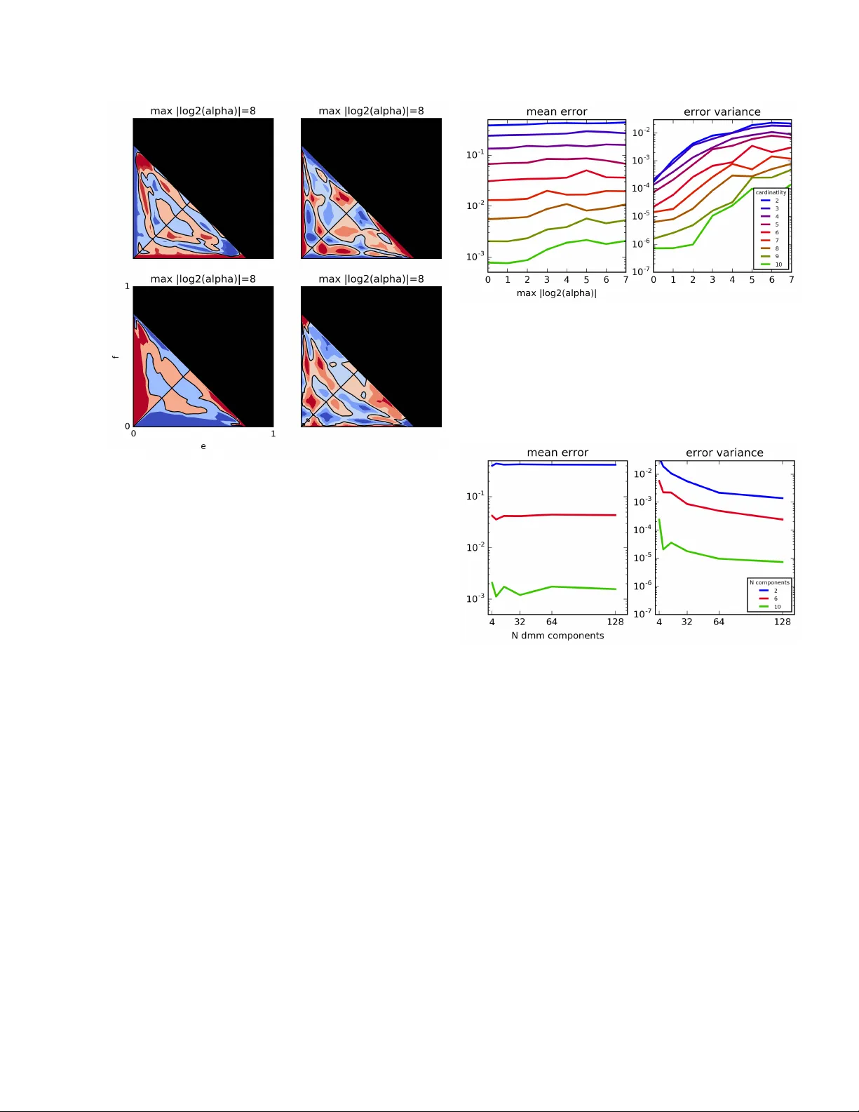
Estimating Causal Dir ection and Conf ounding Of T wo Discr ete V ariables Krzysztof Chalupka Computation and Neural Systems Caltech Frederick Eberhardt Humanities and Social Sciences Caltech Pietro P er ona Electrical Engineering Caltech Abstract W e propose a method to classify the causal re- lationship between two discrete variables gi ven only the joint distribution of the v ariables, ac- knowledging that the method is subject to an in- herent baseline error . W e assume that the causal system is acyclicity , but we do allow for hid- den common causes. Our algorithm presupposes that the probability distributions P ( C ) of a cause C is independent from the probability distrib u- tion P ( E | C ) of the cause-ef fect mechanism. While our classifier is trained with a Bayesian assumption of flat hyperpriors, we do not make this assumption about our test data. This work connects to recent de v elopments on the identifia- bility of causal models o ver continuous v ariables under the assumption of ”independent mech- anisms”. Carefully-commented Python note- books that reproduce all our experiments are av ailable online at vision.caltech.edu/ ˜ kchalupk/code.html . 1 Introduction T ake two discrete variables X and Y that are probabilis- tically dependent. Assume there is no feedback between the v ariables: it is not the case that both X causes Y and Y causes X . Further, assume that any probabilistic depen- dence between variables al ways arises due to a causal con- nection between the variables (Reichenbach, 1991). The fundamental causal question is then to answer two ques- tions: 1) Does X cause Y or does Y cause X ? And 2) Do X and Y have a common cause H ? Since we assumed no feedback in the system, the options in 1) are mutually ex- clusiv e. Each of them, ho we ver , can occur together with a confounder . Fig. 1 enumerates the set of six possible hy- potheses. In this article we present a method to distinguish between these six hypotheses on the basis only of data from the ob- servational joint probability P ( X , Y ) – that is, without re- sorting to experimental interv ention. W ithin the causal graphical models frame work (Pearl, 2000; Spirtes et al., 2000), differentiating between any two of the caus ally interesting possibilities (shown in Fig. 1B- F) is in general only possible if one has the ability to inter- vene on the system. For example, to differentiate between the pure-confounding and the direct-causal case (Fig. 1B and C), one can intervene on X and observ e whether that has an effect on the distribution of Y . Giv en only observa- tions of X and Y and no ability to intervene on the sys- tem howe ver , the problem is in general not identifiable. Roughly speaking, the reason is simply that without any further assumptions about the form of the distribution, any joint P ( X , Y ) can be factorized as P ( X ) P ( Y | X ) and P ( Y ) P ( X | Y ) , and the hidden confounder H can easily be endo wed with a distrib ution that can gi ve the marginal P H P ( X , Y , H ) an y desired form. 2 Related W ork There are two common remedies to the fundamental unidentifiability of the two-variable causal system: 1) Re- sort to interventions or 2) Introduce additional assumptions about the system and derive a solution that works under these assumptions. Whereas the first solution is straight forward, research in the second direction is a more recent and exciting enterprise. 2.1 Additive Noise Models A recent body of work attacks the problem of establish- ing whether x → y or y → x when specific assumptions with respect to the functional form of the causal relation- ship hold. Shimizu et al. (2006) showed for continuous variables that when the effect is a linear function of the cause, with non-Gaussian noise, then the causal direction can be identified in the limit of infinite sample size. This inspired further work on the so called “additi ve noise models”. Hoyer et al. (2009) extended Shimizu’ s identifia- bility results to the case when the effect is any (except for a measure-theoretically small set of) nonlinear function of the cause, and the noise is additi ve – e ven Gaussian. Zhang and Hyv ¨ arinen (2009) showed that a post nonlinear model – that is, y = f ( g ( x ) +  ) where f is an inv ertible func- tion and  a noise term – is identifiable. The additive noise models frame work was applied to discrete variables by Pe- ters et al. (2011). Most of this work has focused on distinguishing the causal orientation in the absence of confounding (i.e. distinguish- ing hypotheses A, C and D in Fig. 1, although Hoyer et al. (2008) hav e extended the linear non-Gaussian methods to the general hypothesis space of Fig, 1 and Janzing et al. (2009) sho wed that the additive noise assumption can be used to detect pure confounding with some success, i.e. to distinguish hypothesis B from hypotheses C and D. The assumption of additi ve noise supplies remarkable iden- tifiability results, and has a natural application in many cases where the variation in the data is thought to deriv e from the measurement process on an otherwise determin- istic functional relation. W ith respect to the more general space of possible probabilistic causal relations it constitutes a very substanti ve assumption. In particular , in the discrete case its application is no longer so natural. 2.2 Bayesian Causal Model Selection From a Bayesian perspectiv e, the question of causal model identification is softened to the question of model selection based on the posterior probability of a causal structure gi ve the data. In a classic work on Bayesian Network learning (then called Belief Net learning), Heckerman and Chick- ering (Heckerman et al., 1995; Chickering, 2002a,b) de- veloped a Bayesian scoring criterion that allowed them to define the posterior probability of each possible Bayesian network given a dataset. Moti vated by results of Geiger and Pearl (1988) and Meek (1995) that showed that for linear Gaussian parameterizations and for multinomial parame- terizations, causal models with identical (conditional) in- dependence structure cannot in principle be distinguished giv en only the observ ational joint distribution over the ob- served variables, their score had the property that it as- signed the same score to graphs with the same indepen- dence structure. But the results of Geiger and Pearl (1988) and Meek (1995) only make an existential claim: That for any joint distribution a parameterization of the appro- priate form exists for any causal structure in the Markov equiv alence class. But one need not conclude from such an existential claim, like Heckerman and Chickering did, that there aren’t reasons in the data that could suggest that one causal structure in a Markov equiv alence class is more probable than another . Thus, the crucial difference between the work of Hecker- mann and ours is that their goal was to find the Markov Figure 1: Possible causal structures linking X and Y . As- sume X, Y and H are all discrete but H is unobserved. In principle, it is impossible to identify the correct causal structure given only X and Y samples. In this report, we will tackle this problem using a minimalistic set of assump- tions. Our final result is a classifier that differentiates be- tween these six cases – the confusion matrices are shown in Fig. 9. Equivalence Class of the true causal model. This, ho wev er, renders our task impossible: all the hypotheses enumerated in Fig. 1B-F are Markov-equi valent. Our contribution is to use assumptions formally identical to theirs (when re- stricted to the causally sufficient case) to assess the likeli- hood of causal structures ov er two observed variables, bear- ing in mind that even in the limit of infinitely many sam- ples, the true model cannot be determined, the structures can only be deemed more or less likely . Our approach is most similar in spirit to the work of Sun et al. (2006). Sun puts an e xplicit Bayesian prior on what a likely causal system is: if X causes Y , then the condition- als p ( Y | X = x ) are less complex than the rev erse con- ditionals P ( X | Y = y ) , where complexity is measured by the Hilbert space norm of the conditional density func- tions. This formulation is plausible and easily applicable to discrete systems (by defining the complexity of discrete probability tables by their entropy). 3 Assumptions Our contrib ution is to create an algorithm with the follo w- ing properties: 1. Applicable to discr ete v ariables X and Y with finitely many states. 2. Decides between all the six possible graphs shown in Fig. 1. 3. Does not make assumptions about the functional form of the discrete parameterization (in contrast to e.g. an additiv e noise assumption). In a recent revie w , Mooij et al. (2014) compares a range of methods that decide the causal direction between two variables, including the methods discussed above. T o our knowledge, none of these methods attempt to distinguish between the pure-causal (A, C, D), the confounded (B), and the causal+confounded case (E,F). W e take an approach inspired by the Bayesian methods discussed in Sec. 2. Consider the Bayesian model in which P ( X , Y ) is sampled from an uninformative hyper- prior with the property that the distribution of the cause is independent of the distribution of the ef fect conditioned on the cause: 1. Assume that P ( ef f ect | cause ) ⊥ ⊥ P ( cause ) . 2. Assume that P ( ef f ect | cause = c ) is sampled from the uninformativ e hyperprior for each c . 3. Assume that P ( cause ) is sampled from the uninfor- mativ e hyperprior . Since all the distributions under considerations are multino- mial, the “uninformati ve hyperprior” is the Dirichlet distri- bution with parameters all equal to 1 (which we will denote as D ir (1) , remembering that 1 is actually a vector whose dimensionality will be clear from conte xt). Which variable is a cause, and which the effect, or whether there is con- founding, depends on which of the causal systems in Fig. 1 are sampled. For e xample, if X → Y and there is also con- founding X ← h → Y (Fig. 1D), then our assumptions set P ( X ) ∼ D ir (1) ∀ x P ( Y | X = x ) ∼ D ir (1) P ( H ) ∼ D ir (1) ∀ h P ( X | H = h ) ∼ D ir (1) ∀ h P ( Y | H = h ) ∼ D ir (1) 4 An Analytical Solution: Causal Direction Consider first the problem of identifying the causal direc- tion. That is, assume that either X → Y or Y → X , and there is no confounding. The assumptions of Sec. 3 then allow us to compute, for any given joint P ( X , Y ) (which we will from no w on denote P X Y to simplify nota- tion), the likelihood p ( X → Y | P X Y ) and the likelihood p ( Y → X | P X Y ) . The likelihood ratio allo ws us to decide which causal direction P X Y more likely represents. W e first derive and visualize the likelihood for the case of X and Y both binary variables. Next, we generalize the result to general X and Y . Finally , we analyze experi- mentally ho w sensitive such causal direction classifier is to breaking the assumption of uninformativ e Dirichlet hyper- priors (but keeping the independent mechanisms assump- tion). 4.1 Optimal Classifier for Binary X and Y Consider first the binary case. Let P X =  a 1 − a  and P Y | X =  b 1 − b c 1 − c  . Assume P X is sampled indepen- dently from P Y | X , and that the densities (parameterized by a and b, c ) are F a , F b , F c : (0 , 1) → R . This de- fines a density ov er ( a, b, c ) , the three-dimensional pa- rameterization of an x → y system, as F ( a, b, c ) = F a ( a ) F b ( b ) F c ( c ) : (0 , 1) 3 → R . Now , consider P X Y =  d e f 1 − ( d + e + f )  – a three- dimensional parameterization of the joint. If we assume that P X Y is sampled according to the X → Y sampling procedure, we can compute its density H X Y : (0 , 1) 3 → R as a function of F using the multiv ariate change of vari- ables formula. W e hav e   d e f   =   ab a (1 − b ) (1 − a ) c   and the in verse transformation is   a b c   =   d + e d d + e f 1 − d − e   (1) The Jacobian of the in verse transformation is d ( a, b, c ) d ( d, e, f ) =    1 1 0 e ( d + e ) 2 − d ( d + e ) 2 0 f (1 − d − e ) 2 f (1 − d − e ) 2 1 1 − d − e ,    its determinant det  d ( a,b,c ) d ( d,e,f )  = − 1 ( d + e ) − ( d + e ) 2 . The change of variables formula then gi ves us H X Y ( d, e, f ) = F ( d + e, d d + e , f 1 − d − e ) ( d + e ) − ( d + e ) 2 , where a, b, c are obtained from Eq. (1). W e can repeat the same reasoning for the inv erse causal direction, Y → X . In this case, we obtain H Y X ( d, e, f ) = F ( d + f , d d + f , e 1 − d − f ) ( d + f ) − ( d + f ) 2 . Giv en P X Y and the hyperpriors F , we can now test which causal direction P X Y most likely corresponds to. Assum- ing equal priors on both causal directions, we hav e p ( X → Y | ( d, e, f )) p ( Y → X | ( d, e, f )) = H xy ( d, e, f ) H y x ( d, e, f ) = F  d + e, d d + e , f 1 − d − e  F  d + f , d d + f , e 1 − d − f  ( d + f ) − ( d + f ) 2 ( d + e ) − ( d + e ) 2 Figure 2: Log likelihood-ratio log  P ( X → Y | ( d,e,f )) P ( Y → X | ( d,e,f ))  as a function of e, f for nine different va lues of d . Red cor- responds to values larger than 0 — that is, X → Y is more likely than the opposite causal direction in the red re- gions. Blue signifies the opposite. The decision boundary is shown in black. It is a union of two orthogonal planes that cut the ( d, e, f ) simplex into four connected compo- nents along a ske wed axis. Only the first factor in the likelihood ratio depends on the hyperprior F . If we fix F a , F b , F c to all be D ir (1) , the factor reduces to 1 and the likelihood ratio becomes p ( X → Y | ( d, e, f )) p ( Y → X | ( d, e, f )) = ( d + f ) − ( d + f ) 2 ( d + e ) − ( d + e ) 2 . Denote the “uninformativ e-hyperprior likelihood ratio” function LR : P X Y ( d, e, f ) 7→ ( d + f ) − ( d + f ) 2 ( d + e ) − ( d + e ) 2 . The classifier that assigns the X → Y class to P X Y with LR ( P X Y ) > 1 , and the Y → X class otherwise is the optimal classifier under our assumptions. Fig.2 sho ws LR across the three-dimensional P X Y simplex. The figure shows nine slices of this simple x for dif ferent values of the d coordinate. 4.2 Optimal Classifier for Arbitrary X and Y Deriving the optimal classifier for the case where X and Y are not binary is analogous to the binary deriv ation. The resulting likelihood ratio is p ( X → Y | P X Y ) p ( Y → X | P X Y ) = (2) = F  P X , P Y | X  F  P Y , P X | Y  | det J X Y | − 1 | det J Y X | − 1 , (3) where J X Y is the Jacobian of the linear transformation ( P X , P Y | X ) 7→ P X Y and J Y X is the Jacobian of the trans- formation ( P Y , P X | Y ) 7→ P X Y . The transformation, its determinant and Jacobian are readily computable on pa- per or using computer algebra systems. In our imple- mentation, we used Theano (Theano Development T eam, 2016) to perform the computation for us. Note that if X has cardinality k X and Y has cardinality k Y , the Jaco- bians have ( k X k Y − 1) 2 entries. Computing their deter- minants has complexity O (( k X k Y − 1) 6 ) or, if we assume k X = k Y = k , O ( k 12 ) – it grows rather quickly with growing cardinality . If F is flat, that is all the priors are D ir (1) , we will call the causal direction classifier that follows Eq. (3) the LR classifier . That is, the LR classifier outputs X → Y if the uninformativ e-hyperprior likelihood ratio is larger than 1, and outputs Y → X otherwise. Note that the optimal classifier is not perfect – there is a baseline error that the optimal classifier has under the as- sumptions it is built on. This error is E LR = Z p ( Y → X | P X Y ) I [ LR ( P X Y ) > 1] + p ( X → Y | P X Y ) I [ LR ( P X Y ) < 1] dP X Y , where the integral varies over all the possible joints P X Y with uniform measure, and I [ LR ( P X Y ) <> 1] is the indicator function that ev aluates to 1 if its subscript condition holds, and to 0 otherwise. That is, assuming that each P X Y is sampled from the un- informativ e Dirichlet prior giv en that either X → Y or Y → X with given probability , in the limit of infinite clas- sification trials the error rate of the LR classifier is E LR . Whereas this integral is not analytically computable (at least neither by the authors nor by a vailable computer alge- bra systems), we can estimate it using Monte Carlo meth- ods in the following sections. In Fig. 6, the leftmost entry on each curv e corresponds to E LR for v arious cardinalities of X and Y . For example, for | X | = | Y | = 2 , E LR ≈ . 4 but already for | X | = | Y | = 10 , E LR < . 001 . 4.3 Robustness: Changing the Hyperprior F What if we use the LR classifier, but our assumptions do not match reality? Namely , what if F is not D ir (1) ? F or example, what if F is a mixture of ten Dirichlet distribu- Figure 3: Samples from Dirichlet mixtures. Each plot shows three random samples from a ten-component mix- ture of Dirichlet distributions over the 1D simplex. Each mixture component has a different, random parameter α . For each plot we fixed a different | l og 2 ( α max ) | , a parame- ter which limits both the smallest and largest value of any of the two α coordinates that define each mixture compo- nent. tions 1 ? W e will dra w F from mixtures with fix ed “ | log 2 ( α max ) | ”. Let the k -th component of the mixture ha ve parameter α k = ( α k 1 , · · · , α k N ) where N is the cardinality of X or Y . Then fixed α max means that we drew each α k i uniformly at random from the interval 2 − α max , 2 α max . Fig. 4 shows samples from such mixtures with growing α max . The fig- ure sho ws that increasing the parameter allo ws the distrib u- tions to grow in comple xity . Note that if α max = 0 , we recover the noninformati ve prior case. How does the likelihood ratio and the causal direc- tion decision boundary change as we allo w α max to depart from 0 ? For binary X and Y , Fig. 4 illustrates the change. Comparing with Fig. 2, we see that as α max grows, the likelihood ratios become more extreme, and the decision boundaries become more complex. Fig. 5 makes it clear that a fixed α max allows for the decision boundary to vary significantly . That the “independent mechanisms” assumption as we framed it is not sufficient to provide identifiability of the causal direction was clear from the outset (since each joint 1 A mixture of Dirichlet distributions with arbitrary many com- ponents can approximate any distrib ution over the simplex. Figure 4: Log-lik elihood ratios for the causal direction when F is a mixture of ten Dirichlet distributions with growing α max (see Fig. 3). can be f actorized as P ( X ) P ( Y | X ) and P ( Y ) P ( X | Y ) ). Howe ver , the above considerations suggest that the as- sumption of noninformati ve hyperpriors is rather strong: In fact, it is possible to show that the decision surface can be precisely flipped with appropriate adjustment of F , making the LR classifier’ s error precisely 100% . Our experiments, ho wev er , suggest that using the LR clas- sifier is a reasonable choice in a wide range of circum- stances, especially as the car dinality of X and Y gr ows . In our experiments, we checked how the error changes as we allow the α max parameter of all the hyperpriors to gro w . Our experimental procedure is as follo ws: 1. Fix the dimensionality of X and Y , and fix α max . 2. Sample 100 h yperpriors for each dimensionality and α max . Sample α parameters for F within giv en α max bounds, where F consists of Dirichlet mixtures (with 10 components), as described abov e. 3. Sample 100 priors for each hyperprior . Sample P ( cause ) and P ( ef f ect | cause ) 100 times for each hyperpriors (that is, for each α setting). 4. Sample the causal label uniformly . If chose X → Y then let P X Y = P ( cause ) P ( ef f ect | cause ) . If chose Y → X , let P X Y = tr anspose [ P ( cause ) P ( ef f ect | cause )] . 5. Classify . Use the LR classifier to classify P X Y ’ s causal direction and record “error” if the causal label disagrees with the classifier . Figure 6 shows the results. As the cardinality of the sys- Figure 5: Log-lik elihood ratios for the causal direction when F is a mixture of ten Dirichlet distributions with | α max | = 2 8 (see Fig. 3) – each plot corresponds to dif- ferent, randomly sampled α . tem grows, the LR classifier’ s decision boundary approx- imates the decision boundary for most Dirichlet mixtures. Another trend is that as α max grows, the variance of the error grows, but there is only a small growing trend in the error itself. In addition, Fig. 7 shows that the error does not increase as we allow more mixture components, up to 128 components, while holding α max at the large value of 7. Thus, the LR classifier performs well e ven for extremely complex hyperpriors, at least on a verage. 5 A Black-box Solution: Detecting Conf ounding Consider now the question of whether X → Y or X → H → Y , where H is a latent variable (a confounder). In this section we present a solution to this problem, under assumptions from Sec. 3. Unfortunately , deriving the optimal classifier for this case is difficult without additional assumptions on the latent H . Instead, we propose a black-box classifier . W e created a dataset of distributions from both the direct-causal and confounded case, using the uninformativ e Dirichlet prior on either P ( X ) and P ( Y | X ) (the direct-causal case) or P ( H ) , P ( X | H ) and P ( Y | H ) in the confounded case. For each confounded distribution, we chose the car- dinality of H , the hidden confounder , uniformly at random between 2 and 100. Next, we trained a neural network to classify the causal structure (Python code that reproduces Figure 6: Results of the direction-classification experi- ment. W e varied cardinality of X , Y as well as α max of the mixture of Dirichlets F . For each setting, we sampled 100 P X Y distributions according to our causal model and recorded the classification error of the s imple LR classifier . The results sho w that, as cardinality of X and Y grows, the LR classifier’ s accuracy increases. Figure 7: Results of the direction-classification experiment when the number of Dirichlet mixture model hyperprior components varies. W e fixed α to vary between 2 − 7 and 2 7 . The results show that the max-likelihood classifier that assumes the noninformative priors is not sensitiv e to the number of Dirichlet mixture components that the test data is sampled from. the experiment is available at vision.caltech.edu/ ˜ kchalupk/code.html ). W e then checked how well this classifier performs as we vary the cardinality of the variables, and as we allow the true hyperprior to be a mix- ture of 10 Dirichlets, analogously to the experiment from Sec. 4. Fig. 8 shows the results. Note that the classification er- rors are much lower than for the “deciding causal direction” case. Both problems (deciding causal direction and detect- ing confounding) are in principle unidentifiable, but it ap- pears the latter is inherently easier . The neural net classifier seems to be little bothered by growing α max . The largest source of error, for cardinality of X and Y larger than 3, seems to be neural network training rather than anything Figure 8: Results of the black-box confounding detec- tor . W e varied cardinality of X , Y as well as α max of the mixture of Dirichlets F . For each setting, we sampled 1000 P X Y distributions according to our causal model and recorded the classification error of a neural net classifier trained on noninformati ve Dirichlet hyperprior data. The results sho w that, as cardinality of X and Y grows, the LR classifier’ s accuracy increases. else. 6 A Black-Box Solution to the General Problem Finally , we present a solution to the general causal discov- ery problem o ver the two v ariables X , Y : deciding between the six alternatives shown in Fig. 1. The idea is a natural extension of the black-box classifier from Sec. 5. W e cre- ated a dataset containing all the six cases, sampled under the assumptions of Sec. 3. W e then trained a neural net- work on this dataset (the neural network architecture, as well as the details of the training procedure, are av ailable in the accompanying Python code). Figure 9 shows the results of applying the classifier to dis- tributions sampled from flat hyperpriors (that is, from a test set with statistics identical to the training set), for cardinal- ities | X | = | Y | = 2 and | X | = | Y | = 10 . As expected, the number of errors is much lower for the higher cardinality . For the cardinality of 2, the confusion matrix shows that the neural networks: 1. easily learn to classify independent vs dependent vari- ables, 2. confuse the X → Y and Y → X cases, and 3. confuse the two “directed-causal plus confounding” cases (Fig. 1E,F). Howe ver , all these are insignificant issues when | X | = 10 , where the total error is 85 out of 10000 testpoints. F or | X | = 2 , the error is 25.7%. W e remark again that the problem is not identifiable – that is, there is no “true causal class” for any point in our training or test dataset. Each distribution could arise from any of the possible fi ve causal Figure 9: Confusion matrices for the all-causal-classes classification task. The test set consists of distributions sampled from uniform hyperpriors – that is, sampled from the same statistics as the training data (equiv alent to α max = 0 in previous sections). A) Results for | X | = | Y | = 2 . T otal number of errors=2477. B) Results for | X | = | Y | = 10 , total errors=85. C) A verage results for | X | = | Y | = 10 , same classifier as in B) but test set sam- pled with non-uniform hyperpriors with α max = 7 (see text). 201 errors on average. In each case, the test set con- tains 10000 distributions, with all the classes sampled with an equal chance. systems in which X and Y are not independent. The fact that the error nears 0 in the high-cardinality case indi- cates that the likelihoods under our assumptions gro w very peaked as the cardinality gro ws. Thus, the optimal decision can quite safely be called the true decision. In addition, Fig. 9C shows the a verage confusion table for a hundred tri- als in which our classifier was applied to distributions ov er X and Y with cardinality 10, corresponding to all the pos- sible six causal structures, but sampled from non-uniform hyperpriors with α max = 7 . The performance drop is not drastic compared to Fig. 9B. 7 Discussion W e dev eloped a neural network that determines the causal structure that links two discrete variables. W e allo w for confounding between the two variables, but assumed acyclicity . The classifier takes as input a joint probability table P X Y between the two variables and outputs the most likely causal graph that corresponds to this joint. The pos- sible causal graphs span the range shown in Fig. 1 - from independence to confounding co-occurring with direct cau- sation. W e emphasize two limitations of the classifier: 1. Since the classifier makes a forced choice between the six ac yclic alternativ es, it will necessarily produce 100% error on P X Y ’ s generated from cyclic systems. 2. Our goal was not, and can not be, to achieve 100% accuracy . For example, error in Fig. 9A is about 25%. Howe ver , this is not necessarily a “bad” result. Our considerations in Sec. 3 and 4 show that even when all our assumptions hold, the optimal classifier has a non-zero error . The latter is a consequence of the non-identifiability of the problem: it is not possible, in general, to identify the causal structure between two v ariables by looking at the joint dis- tribution and without intervention. Our goal was to intro- duce a minimal set of assumptions that, while ackno wledg- ing the nonidentifiability , enable us to make useful infer- ences. W e noted that as the cardinality of the variables raises, the task becomes more and more “identifiable” in the sense that, for each giv en P X Y , one out of the possible six causal graphs strongly dominates the others with respect to its likelihood. In this situation, the most likely causal structure becomes essentially the only possible one, barring a small error , and the problem becomes practically identifiable. All of the above applies assuming that our generati ve model corresponds to reality . The assumptions, discussed in Sec. 3, boil do wn to tw o ideas: 1) The w orld creates causes independently of causal mechanisms and 2) Causes are ran- dom variables whose distributions are sampled from flat Dirichlet hyperpriors. Causal mechanisms are conditional distributions of effects given causes, and are also sampled from flat Dirichlet hyperpriors. Whether these assumptions are realistic or not is an undecidable question. Neverthe- less, through a series of simple experiments (Fig. 6, Fig. 7, Fig. 8, Fig. 9) we sho wed that the assumption of flat hyper - priors is not essential – our classifiers’ average performance does not decrease significantly as we allo w the hyperpriors to vary , although the v ariance of the performance gro ws. In future work, we will carefully analyze under what condi- tions the flat-hyperprior classifier performs well e ven if the hyperpriors are not flat. The current working hypothesis is that as long as the hyperprior on P ( cause ) is the same as the hyperprior on P ( ef f ect | cause ) , the classification performance doesn’t change significantly on average , but –as seen in our experiments – it will have increased vari- ance. Shohei Shimizu explained our task (for the case of con- tinuous variables) as: “Under what circumstances and in what way can one determine causal structure based on data which is not obtained by controlled experiments b ut by pas- siv e observation only?” (Shimizu et al., 2006). Our answer is, “For high-cardinality discrete variables, it seems enough to assume independence of P ( cause ) from P ( ef f ect | cause ) , and train a neural network that learns the black-box mapping between observations and their causal generativ e mechanism. ” References David Maxwell Chickering. Learning equiv alence classes of bayesian-network structures. J ournal of machine learning r esearc h , 2(Feb):445–498, 2002a. David Maxwell Chickering. Optimal structure identifica- tion with greedy search. Journal of machine learning r esearc h , 3(Nov):507–554, 2002b. D. Geiger and J. Pearl. On the logic of causal models. In Pr oceedings of U AI , 1988. David Heckerman, Dan Geiger , and David M Chickering. Learning bayesian networks: The combination of kno wl- edge and statistical data. Machine learning , 20(3):197– 243, 1995. Patrik O Hoyer , Dominik Janzing, Joris M Mooij, Jonas Pe- ters, and Bernhard Sch ¨ olkopf. Nonlinear causal discov- ery with additive noise models. In Advances in neural information pr ocessing systems , pages 689–696, 2009. P .O. Hoyer , S. Shimizu, A.J. Kerminen, and M. P alviainen. Estimation of causal effects using linear non-Gaussian causal models with hidden v ariables. International Jour - nal of Appr oximate Reasoning , 49:362–378, 2008. Dominik Janzing, Jonas Peters, Joris Mooij, and Bernhard Sch ¨ olkopf. Identifying confounders using additi ve noise models. In Pr oceedings of the T wenty-F ifth Confer ence on Uncertainty in Artificial Intellig ence , pages 249–257. A UAI Press, 2009. C. Meek. Strong completeness and faithfulness in Bayesian networks. In Eleventh Confer ence on Uncertainty in Ar- tificial Intelligence , pages 411–418, 1995. Joris M Mooij, Jonas Peters, Dominik Janzing, Jakob Zscheischler , and Bernhard Sch ¨ olkopf. Distinguishing cause from ef fect using observational data: methods and benchmarks. arXiv preprint , 2014. J. Pearl. Causality: Models, Reasoning and Infer ence . Cambridge Univ ersity Press, 2000. Jonas Peters, Dominik Janzing, and Bernhard Scholkopf. Causal inference on discrete data using additive noise models. IEEE T ransactions on P attern Analysis and Ma- chine Intelligence , 33(12):2436–2450, 2011. Hans Reichenbach. The dir ection of time , v olume 65. Univ of California Press, 1991. Shohei Shimizu, Patrik O Hoyer , Aapo Hyv ¨ arinen, and Antti Kerminen. A linear non-gaussian acyclic model for causal discovery . Journal of Machine Learning Re- sear ch , 7(Oct):2003–2030, 2006. P . Spirtes, C. N. Glymour , and R. Scheines. Causation, pr ediction, and searc h . Massachusetts Institute of T ech- nology , 2nd ed. edition, 2000. Xiaohai Sun, Dominik Janzing, and Bernhard Sch ¨ olkopf. Causal inference by choosing graphs with most plausible markov k ernels. In ISAIM , 2006. Theano Dev elopment T eam. Theano: A Python frame work for fast computation of mathematical expressions. arXiv e-prints , abs/1605.02688, May 2016. URL http:// arxiv.org/abs/1605.02688 . Kun Zhang and Aapo Hyv ¨ arinen. On the identifiability of the post-nonlinear causal model. In Pr oceedings of the twenty-fifth confer ence on uncertainty in artificial intel- ligence , pages 647–655. A UAI Press, 2009.