Sampling and Estimation for (Sparse) Exchangeable Graphs

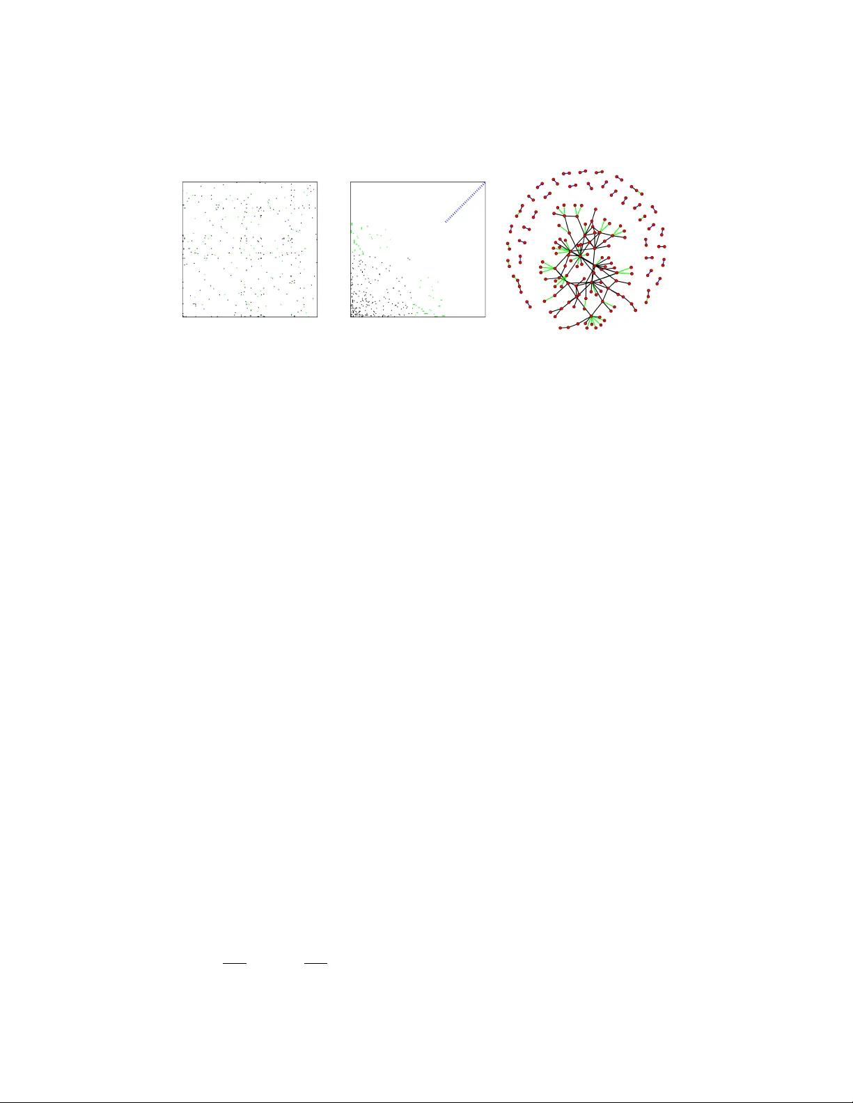
SAMPLING AND ESTIMA TION F OR (SP ARSE) EX CHANGEABLE GRAPHS VICTOR VEITCH AND DANIEL M. R O Y Abstract. Sparse exchangeable graphs on R + , and the asso ciated graphex framework for sparse graphs, generalize exc hangeable graphs on N , and the associated graphon framework for dense graphs. W e develop the graphex framework as a to ol for statistical netw ork analysis by identifying the sampling scheme that is naturally asso ciated with the mo dels of the framework, and by introducing a general consistent estimator for the parameter (the graphex) underlying these models. The sampling sc heme is a mo dification of indep enden t vertex sampling that throws aw ay vertices that are isolated in the sampled subgraph. The estimator is a dilation of the empirical graphon estimator, which is kno wn to be a consistent estimator for dense exchangeable graphs; both can be understoo d as graph analogues to the empirical distribution in the i.i.d. sequence setting. Our results may b e viewed as a generalization of consistent estimation via the empirical graphon from the dense graph regime to also include sparse graphs. Contents 1. In tro duction 1 2. Preliminaries 8 3. Sampling 10 4. Estimation with kno wn sizes 11 5. Estimation for unkno wn sizes 21 A ckno wledgements 25 References 25 1. Intr oduction This pap er is concerned with mathematical foundations for the statistical analysis of real-w orld net w orks. F or densely connected net w orks, the graphon framework has emerged as p o w erful to ol for b oth theory and applications in net w ork analysis; man y of the mo dels used in practice are within the remit of this framework (see [ OR15 ] for a review). Ho wev er, in most real-w orld situations, net w orks are sparsely connected; i.e., as one studies larger netw orks, one finds that they tend to exhibit only a v anishing fraction of all p ossible links. In this pap er, we con tin ue our study of sparse exchangeable graphs, i.e., random graphs whose vertices may b e iden tified with nonnegative reals, R + , and whose edge sets are then mo deled b y exchangeable p oin t pro cesses on R 2 + . In a pioneering pap er, Caron and F o x [ CF14 ] in troduced the notion of sparse exchangeable graphs in the con text of nonparametric Ba yesian analysis. Building on this work, the general family of all sparse exchangeable graphs was characterized b y V eitch and Roy [ VR15 ]; Borgs, Cha yes, Cohn, and Holden [ BCCH16 ], and shown to generalize the graphon mo dels for dense graphs to include the sparse graph regime. Sparse exc hangeable graphs ha ve a n um b er of desirable prop erties, including that they define a natural pro jective 1 SAMPLING AND ESTIMA TION FOR (SP ARSE) EXCHANGEABLE GRAPHS 2 family of subgraphs of gro wing size, which can b e used to model the process of observing a larger and larger fraction of a fixed underlying netw ork. This prop erty also provides a firm foundation for the study of v arious asymptotics, as demonstrated b y [ VR15 ; BCCH16 ] and the results here. [ VR15 ] characterized the asymptotic degree distribution and connectedness of sparse exchangeable graphs, demonstrating that sparse exchangeable graphs allow for sparsity and admit the ric h graph structure (suc h as small-world connectivity and p o w er la w degree distributions) found in large real-w orld netw orks. On this basis, V eitc h and Ro y argue that sparse exc hangeable graphs can serv e as a general statistical mo del for net work data. Despite our understanding of these mo dels, the statistical meaning remains somewhat opaque. Put simply , when w ould it be natural to use the sparse exc hangeable graph model? The present pap er further dev elops this framework for statistical netw ork analysis b y answering tw o fundamen tal questions: (1) What is the notion of sampling naturally asso ciated with this statistical net work model? and (2) Ho w can w e use an observ ed dataset to consistently estimate the statistical net work model? The answers to these questions significan tly clarify b oth the meaning of the mo deling framew ork, and its connection to the dense graph framework and the classical i.i.d. sequence framework at the foundation of classical statistics. These questions ma y b e viewed as sp ecific examples of a general approac h to formalizing the problem of statistical analysis on net work data b eing carried out b y Orbanz [ Orb16 ]. T o explain the results, we first recall the mo deling framework of [ VR15 ; BCCH16 ]. The basic setup introduces a family of finite, symmetric p oin t pro cesses Γ s ⊆ [0 , s ] × [0 , s ] , for s ∈ R + , where each Γ s is interpreted as the edge set of a random graph whose vertices are p oints in the in terv al [0 , s ] . Hence, for θ , θ 0 ∈ [0 , s ] , there is an edge betw een θ and θ 0 if and only if ( θ , θ 0 ) ∈ Γ s . The edge set Γ s determines a graph ov er its activ e v ertex set: those elements θ ∈ [0 , s ] such that θ exhibits some edge in Γ s . A ccordingly , (Γ s ) s ∈ R + are understo o d as ( R + -lab eled) graph-v alued random v ariables that are nested in the sense that Γ r ⊆ Γ s whenev er r ≤ s . W e will argue below that the indices s ∈ R + are prop erly understo o d as sp ecifying the sample size of the corresp onding observ ations Γ s . The natural parameter of the distributions of these graphs is a gr aphex W = ( I , S, W ) defined on some lo cally finite measure space ( ϑ , B ϑ , ν ) where I ∈ R + , S : ϑ → R + is an in tegrable function, and W : ϑ 2 → [0 , 1] is a symmetric function satisfying several weak in tegrability conditions we formalize later. (Without loss of generalit y , one can alw ays take ( ϑ , B ϑ ) to b e the non-negative reals, R + , with its standard Borel structure, and take ν to b e Leb esgue measure Λ .) The comp onen t W is a natural generalization of the graphon of the dense graph mo dels [ VR15 ; BCCH16 ], and for this reason we refer to it as a gr aphon . Although the results of the present pap er hold for general graphexes, for simplicity of exp osition, w e will temp orarily restrict our atten tion to graphexes of the form W = (0 , 0 , W ) , giving a full treatment in subsequent sections. W e b egin by giving a construction of the graphex pro cess for a graphex of the form W = (0 , 0 , W ) : Let Π be a P oisson (p oin t) pro cess on R + × ϑ with intensit y Λ ⊗ ν , i.e., for tw o interv als J 1 , J 2 ⊆ R + and tw o measurable subsets B 1 , B 2 ⊆ ϑ , the num ber of p oints of Π in J 1 × B 1 and in J 2 × B 2 are Poisson random v ariables with mean | J 1 | ν ( B 1 ) and | J 2 | ν ( B 2 ) resp ectively , where | J i | = Λ( J i ) is the length of SAMPLING AND ESTIMA TION FOR (SP ARSE) EXCHANGEABLE GRAPHS 3 the interv al, and these v ariables are ev en indep enden t when J 1 × B 1 ∩ J 2 × B 2 = ∅ . (If ν is also Leb esgue measure on R + , then Π is then simply a unit-rate Poisson pro cess on R 2 + .) W rite { ( θ i , ϑ i ) } i ∈ N for the points of Π , let Π s b e the restriction of Π to [0 , s ] 2 , and let ( ζ { i,j } ) i ≤ j ∈ N b e an i.i.d. collection of uniform random v ariables in [0 , 1] . F or every s ∈ R + , define the size- s random edge set Γ s on [0 , s ] to be exactly the set of distinct pairs ( θ i , θ j ) where θ i , θ j ≤ s and ζ { i,j } ≤ W ( ϑ i , ϑ j ) . In other words, for every distinct pair of points ( θ , ϑ ) , ( θ 0 , ϑ 0 ) ∈ Π s , the edge set Γ s includes the edge ( θ , θ 0 ) indep enden tly with probability W ( ϑ, ϑ 0 ) . The vertex set of the graph corresp onding to the edge set Γ s is defined to b e those p oints that app ear in some edge; hence, this mo del does not allow for isolated v ertices. The entire family of graphs Γ s , for s ∈ R + , is a pro jective family with respect to subset restriction, i.e., Γ r = Γ s ∩ [0 , r ] 2 for every r , s ∈ R + with r ≤ s . See Fig. 1 for an illustration of the generativ e mo del for a general graphex W defined on R + with Leb esgue measure. A rigorous definition is provided in Section 2 . W e refer to Γ as the gr aphex pr o c ess generated b y W : we also use this nomencla- ture for the family (Γ s ) s ∈ R + . Note that the Γ has the prop erty that its distribution is in v ariant to the action of the maps ( x, y ) 7→ ( φ ( x ) , φ ( y )) , where φ : R + → R + is mea- sure preserving. A random graph with this property is called a sparse exc hangeable graph [ CF14 ]. In Section 2 , we quote the result due to V eitch and Roy [ VR15 ]; Borgs, Cha yes, Cohn, and Holden [ BCCH16 ], building off w ork by Kallenberg [ Kal90 ], that pro ves that every (sparse) exchangeable graph is a graphex pro cess generated b y some (p oten tially random) graphex. F or a finite lab eled graph G , such as each Γ s , for s ∈ R + , we will write G ( G ) to denote the unlab ele d 1 graph corresp onding to G . The first con tribution of the present pap er is the iden tification of a sampling sc heme that is naturally asso ciated with the graphex pro cesses: Definition 1.1. A p -sampling of an unlab eled graph G is obtained by selecting eac h vertex of G indep enden tly with probability p ∈ [0 , 1] , and then returning the edge set of the random v ertex-induced subgraph of G . It is imp ortan t to note that only the edge set of the vertex-induced subgraph is returned; in other words, v ertices that are isolated from the other sampled vertices are thrown a wa y . The key fact ab out this sampling scheme is that: F or s > 0 and r ∈ [0 , s ] , if G r is an r /s -sampling of G (Γ s ) then G r d = G (Γ r ) . This result justifies the interpretation of the parameter s as a sample size. In the estimation problem for the graphex pro cess, the observ ed dataset is a realization of the random sequence of graphs G 1 , G 2 , . . . suc h that G k = G (Γ s k ) , and s 1 , s 2 , . . . is some sequence of sizes suc h that s k ↑ ∞ as k → ∞ . The task is to tak e suc h an observ ation and return an estimate for W , where W is the graphex that generated (Γ s ) s ∈ R + . Both the form ulation and solution of this problem depend on whether the sizes s k are included as part of the observ ations. W e first treat the simpler case where the sizes are kno wn. T o formalize the estimation problem w e m ust in tro duce a notion of when one graphex is a go od appro ximation for another. In tuitiv ely , our notion is that, for an y fixed s , a size- s 1 The unlab elled graph corresp onding to a lab elled graph G is the equiv alence class of graphs isomorphic to G . Restricting ourselv es to finite unlab elled graphs, we can represent the unlab elled graphs formally in terms of their homomorphism counts, ( N F ) , where F ranges o ver the countable set of all finite simple graphs whose vertex set is [ n ] for some n ∈ N , and N F is the num b er of homomorphisms from F to G . SAMPLING AND ESTIMA TION FOR (SP ARSE) EXCHANGEABLE GRAPHS 4 s t ϑ 8 θ 8 ϑ 2 θ 2 ϑ 1 θ 1 ϑ 9 θ 9 ϑ 4 θ 4 ϑ 3 θ 3 s t s s t t θ 8 θ 8 θ 2 θ 2 θ 1 θ 1 θ 9 θ 9 θ 4 θ 4 θ 3 θ 3 0 s t Figure 1. Generativ e pro cess of a graphex pro cess generated by a graphex W = ( I , S, W ) defined on R + with Leb esgue measure, observed at sizes s and t . First panel: a (necessarily truncated) realization of the latent P oisson pro cess Π t on [0 , t ] × R + . A coun tably infinite num b er of p oin ts lie ab o ve the six p oin ts visualized. Second panel: Edges due to the graphon comp onent W are sampled by connecting eac h distinct pair of p oin ts ( θ i , ϑ i ) , ( θ j , ϑ j ) ∈ Π t indep enden tly with probability W ( ϑ i , ϑ j ) . Integrabilit y conditions on W imply that only a finite n um b er of edges will app ear, despite there b eing an infinite num ber of p oin ts in Π t . Assume the three edges are the only ones. Third panel: The edge set Γ t represen ted as an adjacency measure on [0 , t ] 2 . The edges in the graphon comp onent app ears as (symmetric pairs of ) black dots; the edges corresp onding to the star comp onen t S app ear in green; the isolated edges (from the I comp onen t) appear in blue. At size s , only the edges in [0 , s ] 2 (inner dashed black line) appear in the graph. The edges { θ j , σ j k } of the star ( S ) comp onent of the pro cess (green) centered at θ j are realizations of a rate- S ( ϑ j ) Poisson pro cess { σ j k } along the line through θ j (sho w as green dots along grey dotted lines). Hence, at size t , eac h point θ i is the center of P oi ( t S ( ϑ i )) star process rays. The edges { ρ i , ρ 0 j } generated b y the isolated edge ( I ) component of the pro cess (blue) are a realization of a rate- I Poisson pro cess on the upp er (or lo wer) triangle of [0 , t ] 2 , reflected. A t size t , there are P oi ( t 2 I ) isolated edges due to this part of the graphex. The final panel sho ws the graphs corresp onding to the sampled adjacency measure at sizes s and t . random graph generated by an estimator should b e close in distribution to a size- s random graph generated by the true graphex. Let uKEG ( W , s ) b e the distribution of an unlab eled size- s graphex pro cess, i.e., the distribution of G (Γ s ) where Γ is generated b y W . Appro ximation is then formalized by the following notion of con vergence: Definition 1.2. W rite W k → GP W as k → ∞ , when uKEG ( W k , s ) → uKEG ( W , s ) w eakly as k → ∞ , for all s ∈ R + . Our goal in the estimation problem is then to take a sequence of observ ations and use these to pro duce a sequence of graphexes W 1 , W 2 , . . . that are consistent in the sense that W k → GP W as k → ∞ . This is a natural analogue of the definition of consistent estimation used for the conv ergence of the empirical cumulativ e distribution function in the i.i.d. sequence setting, and of the definition of consisten t estimation used for the conv ergence of the empirical graphon in the dense graph setting. Let v ( G ) denote the num ber of vertices of graph G . Our estimator is the dilate d empiric al gr aphon ˆ W ( G k ,s k ) : [0 , v ( G k ) /s k ) 2 → { 0 , 1 } , (1.1) SAMPLING AND ESTIMA TION FOR (SP ARSE) EXCHANGEABLE GRAPHS 5 defined by transforming the adjacency matrix of G k in to a step function on [0 , v ( G k ) /s k ) 2 where eac h pixel has size 1 /s k × 1 /s k ; see Fig. 2 . Intuitiv e ly , when the generating graphex is W = (0 , 0 , W ) , we ha ve s k ↑ ∞ as k → ∞ , and the estimator is an increasingly higher and higher resolution pixel picture of the generating graphon. F ormally , given a non-empt y finite graph G with n v ertices labeled 1 , . . . , n , we define the empirical graphon ˜ W G : [0 , 1] 2 → { 0 , 1 } b y partitioning [0 , 1] into adjacen t in terv als I 1 , . . . , I n eac h of length 1 /n and taking ˜ W G = 1 on I i × I j if i and j are connected in G , and taking ˜ W = 0 otherwise. The dilated empirical graphon with dilation s is then defined by ˆ W ( G,s ) ( x, y ) = ˜ W G ( x/s, y /s ) . T o map an unlab eled graph to a (dilated) empirical graphon we must introduce a lab eling of the v ertices. Notice that if φ : R + → R + is a measure-preserving transformation, φ ⊗ φ is the map ( φ ⊗ φ )( x, y ) = ( φ ( x ) , φ ( y )) , W = ( I , S, W ) , and W 0 = ( I , S ◦ φ, W ◦ ( φ ⊗ φ )) , then uKEG ( W , s ) = uKEG ( W 0 , s ) for all s ∈ R + . In particular, the dilated empiri- cal graphon functions corresponding to differen t lab elings of the v ertices of G are related by obvious measure-preserving transformations in this wa y . F or the purp oses of this pap er, graphexes that give rise to the same distributions ov er graphs are equiv alent. W e then define the empirical graphon of an unlabeled graph to b e the empirical graphon of that graph with some arbitrary lab eling, and we define the dilated empirical graphon similarly . These functions may b e thought as arbitrary represen tatives of the equiv alence class on graphons giv en by equating t w o graphons whenev er they correspond to isomorphic graphs. The first main estimation result is that ˆ W ( G k ,s k ) → GP W in probability as k → ∞ . That is, for every infinite sequence N ⊆ N there is a further infinite subsequence N 0 ⊆ N suc h that ˆ W ( G k ,s k ) → GP W almost surely along N 0 . Sub ject to an additional technical constraint (implied by integrabilit y of W ) the con vergence in probability may b e replaced b y conv ergence almost surely . Note that consistency holds for observ ations generated by an arbitrary graphex W = ( I , S, W ) , not just those with the form W = (0 , 0 , W ) ; see Fig. 3 . W e now turn to the setting where the observ ation sizes s 1 , s 2 , . . . are not included as part of the observ ations. In this case, w e study tw o natural mo dels for the dataset. The first is to treat the observed graphs G k as realizations of G (Γ s k ) for some (unkno wn) sequence s k ↑ ∞ as k → ∞ that is indep enden t of Γ . Another natural mo del is to take G 1 , G 2 , . . . to b e the sequence of all distinct graph structures tak en on by (Γ s ) s ∈ R + ; in this case, for all k , we tak e G k = G (Γ τ k ) , where τ k is the laten t size at the k th o ccasion that the graph structure c hanges. In this later case, w e call G (Γ) = ( G (Γ τ 1 ) , G (Γ τ 2 ) , . . . ) the graph sequence of Γ . (W e define the graph sequence formally in Section 2 .) In tuitively , G (Γ) is the graphex pro cess Γ with the size information stripp ed a wa y . In this sense, the graph sequence of Γ is the random ob ject naturally associated to W when the sizes are unobserv ed. Thus, in this setting, con v ergence in distribution of the graph sequences induced by the estimators is a natural notion of consistency . Definition 1.3. W rite W k → GS W as k → ∞ when G (Γ k ) d − → G (Γ) as k → ∞ , for Γ k generated by W k and Γ generated by W . The notion of consisten t estimation corresp onding to this conv ergence is that, for any fixed  ∈ N , the distribution of the length  prefix of the graph sequence generated b y the estimator should b e close to the distribution of the length  prefix of the graph sequence generated b y W . Conv ergence in distribution of every finite-size prefix is equiv alen t to con v ergence in distribution of the en tire sequence. SAMPLING AND ESTIMA TION FOR (SP ARSE) EXCHANGEABLE GRAPHS 6 Figure 2. Realizations of dilated empirical graphons of graphex processes generated b y (0 , 0 , W ) for W giv en in the rightmost column, at observ ation sizes given in the b ottom ro w. Note that the ordering of the vertices used to define the estimator is arbitrary . Here w e ha ve suggestiv ely ordered the vertices according to the laten t v alues from the process simulations; with this ordering the dilated empirical graphons are appro ximate pixel pictures of the generating graphon where the resolution b ecomes finer as the observ ation size grows. All three graphons satisfy k W k 1 = 1 , and thus the exp ected n um b er of edges (black pixels) at each size s is 1 2 s 2 in each column. Note that the rate of dilation is faster for sparser graphs; as established in [ VR15 ], the topmost graphex process used for this example is sparser than the middle graphex pro cess, and the graphon generating the b ottom graphex pro cess is compactly supp orted and thus corresp onds to a dense graph. T o explain our estimator for this setting, w e will need the following concept: Definition 1.4. Let c ∈ R + and let W = ( I , S, W ) b e a graphex. A c -dilation of W is the graphex W c = ( c 2 I , cS ( · /c ) , W ( · /c, · /c )) . The k ey fact ab out c -dilations is that uKEG ( W , s ) = uKEG ( W c , s/c ) for all s ∈ R + , and thus also G (Γ) d = G (Γ c ) whenever Γ is generated b y W and Γ c is generated b y W c . That is, the law of the graph sequence is inv ariant to dilations of the generating graphex. This means, in particular, that the dilation of a graphex is not an identifiable parameter when the observ ation sizes are not included as part of the observ ation. The obvious guess for the estimator in this setting is then the estimator for the kno wn-sizes setting with the dilation information stripp ed aw ay . That is, our estimator is the dilated empirical graphon mo dulo dilation; i.e., it is simply the empirical graphon ˜ W G k : [0 , 1] 2 → [0 , 1] defined abov e. In this setting, the empirical graphon is acting as a representativ e of its equiv alence class under the relation that equates graphons that generate graph sequences with the same la ws. The main estimation result is that if either (1) There is some (p ossibly random) sequence ( s k ) , indep enden t from Γ , such that s k ↑ ∞ a.s. and G k = G (Γ s k ) for all k ∈ N , or (2) ( G 1 , G 2 , . . . ) = G (Γ) , SAMPLING AND ESTIMA TION FOR (SP ARSE) EXCHANGEABLE GRAPHS 7 Figure 3. Realization of unlab eled graphex pro cess generated by W = ( I , S, W ) at size s = 15 (righ t panel), and asso ciated dilated empirical graphon (left and cen ter panels). The generating graphex is W = ( x + 1) − 2 ( y + 1) − 2 , S = 1 / 2 exp ( − ( x + 1)) , and I = 0 . 1 . The observ ation size is s = 15 . The dilated empirical graphex is pictured as tw o equiv alent representations ˆ W ( G, 15) and ˆ W 0 ( G, 15) , eac h with supp ort [0 , 12) 2 ( 180 v ertices at size 15 ). Edges from the W comp onen t are shown in black, edges from the S comp onen t are shown in green, and edges from the I comp onen t are sho wn in blue. Recall that the ordering of the dilated empirical graphon is arbitrary , so the left and center panels depict different representations of the same estimator. The leftmost panel shows the dilated empirical graphon with a random ordering. The middle panel shows the dilated empirical graphon sorted to group the I , S , and W edges, with the W edges sorted as in Fig. 2 . The middle panel giv es some intuition for why the dilated empirical graphon is able to estimate the en tire graphex triple: When a graphex pro cess is generated according to ˆ W ( G, 15) with laten t P oisson process Π , the disjoint structure of the dilated graphon regions due to the I , S , and W comp onen ts induces a natural partitioning of Π into indep enden t Poisson pro cesses that repro duce the indep endence structure used in the full generative mo del Eq. ( 2.1 ). then ˜ W G k → GS W in probabilit y as k → ∞ . Sub ject to an additional techni- cal constrain t (implied by integrabilit y), the conv ergence in probability ma y be strengthened to con v ergence almost surely . Our estimation results are inspired by Kallenberg’s dev elopment of the theory of estimation for exc hangeable arrays [ Kal99 ]. Restricted to the graph setting (that is, 2 -dimensional arrays interpreted as adjacency matrices), and translated into mo dern language, that pap er introduced the empirical graphon (although not named as such) and formalized consistency in terms of the weak top ology: W k → W as k → ∞ when the graphs generated b y W k con verge in distribution to the graphs generated b y W . The estimation results of the presen t pap er may be seen as generalizations of [ Kal99 ] to the sparse graph regime. The presen t paper is also closely related to the recen t pap er [ BCCH16 ]. Spe- cialized to the case ϑ = R + equipp ed with Leb esgue measure, that paper extends the cut distance betw een compactly supp orted graphons—a core tool in the limit theory of dense graphs —to arbitrary in tegrable graphons. Conv ergence in the cut distance then gives a notion of limit for sequences of graphons. This is ex- tended to a notion of conv ergence for sequences of (sparse) graphs by sa ying that a sequence G 1 , G 2 , . . . con verges in the stretc hed cut distance sen se if and only if ˆ W ( G 1 , √ e ( G 1 ) , ˆ W ( G 2 , √ e ( G 2 ) , . . . con verges with respect to the cut distance. That is, SAMPLING AND ESTIMA TION FOR (SP ARSE) EXCHANGEABLE GRAPHS 8 eac h graph G k is mapp ed to the empirical graphon dilated b y v ( G k ) / p e ( G k ) . The same pap er also establishes that e ( G k ) /s 2 k → k W k 1 a.s. . Thus, in the k W k 1 = 1 case, these dilated empirical graphons, considered as pixel pictures, will look asymptoti- cally identical to the v ( G k ) /s k -dilated empirical graphons that w e use as estimators in the known sizes case. This suggests that a close connection b etw een consisten t estimation and con v ergence in the cut distance. Indeed, in the dense graph setting these notions of con v ergence are kno wn to b e equiv alen t (in the dense setting, the con vergence W k → GP W as k → ∞ is equiv alent to left con v ergence [ DJ08 ], and left conv ergence is equiv alence to conv ergence in the cut norm [ BCLS+08 ]). An analogous result in the sparse graph setting would allow for a very different approach to proving our conv ergence result in the kno wn size setting, restricted to the special case that the generating graphex is an integrable graphon. The pap er is organized as follows: In Section 2 we give formal definitions for the basic to ols of the paper. The sampling result is d eriv ed in Section 3 . In Section 4 w e prov e the estimation result for the setting where observ ation sizes are included as part of the observ ation. W e build on this in Section 5 to pro ve the estimation result for the setting where the true underlying observ ation sizes are not observed. 2. Preliminaries The basic ob ject of in terest in this pap er is p oint pro cesses on R 2 + , interpreted as the edge sets of random graphs with vertices lab eled in R + . Definition 2.1. An adjac ency me asur e is a purely atomic, symmetric, simple, lo cally finite measure on R 2 + . If ξ = P i,j δ ( θ i ,θ j ) is an adjacency measure then the asso ciated graph with lab els in R + is one with edge set { ( θ i , θ j ) } , where θ i ≤ θ j ; the vertex set is deduced from the edge set. The defining prop ert y of graphex pro cesses is that, intuitiv ely sp eaking, the lab els of the vertices of the graph are uninformative ab out the graph structure. This is formalized by requiring that the asso ciated adjacency measure is join tly exc hangeable, where Definition 2.2. A random measure ξ on R 2 + is jointly exchange able if ξ ◦ ( φ ⊗ φ ) d = ξ for any measure-preserving transformation φ : R + → R + . A representation theorem for join tly exchangeable random measures on R 2 + w as giv en b y Kallenberg [ Kal05 ; Kal90 ]. This result w as translated to the setting of ran- dom graphs in [ VR15 ]. W riting Λ for Leb esgue measure and µ W ( · ) = ´ R + W ( x, · )d x , the defining ob ject of the representation theorem is: Definition 2.3. A gr aphex is a triple ( I , S, W ) , where I ≥ 0 is a non-negativ e real, S : R + → R + is integrable, and the gr aphon W : R 2 + → [0 , 1] is symmetric, and satisfies (1) Λ { µ W = ∞} = 0 and Λ { µ W > 1 } < ∞ , (2) Λ 2 [ W ; µ W ∨ µ W ≤ 1] = ´ R 2 + W ( x, y ) 1[ µ W ( x ) ≤ 1] 1[ µ W ( y ) ≤ 1]d x d y < ∞ , (3) ´ R + W ( x, x ) d x < ∞ . W e say that a graphex is non-trivial if I + k S k 1 + k W k 1 > 0 , i.e. if it is not the case that the graphex is 0 a.e. The representation theorem is: SAMPLING AND ESTIMA TION FOR (SP ARSE) EXCHANGEABLE GRAPHS 9 Theorem 2.4. L et ξ b e a r andom adjac ency me asur e. ξ is jointly exchange able iff ther e exists a (p ossibly r andom) gr aphex W = ( I , S, W ) such that, almost sur ely, ξ = X i,j 1[ W ( ϑ i , ϑ j ) ≤ ζ { i,j } ] δ θ i ,θ j + X j,k 1[ χ j k ≤ S ( ϑ j )]( δ θ j ,σ j k + δ σ j k ,θ j ) + X k 1[ η k ≤ I ]( δ ρ k ,ρ 0 k + δ ρ 0 k ,ρ k ) , (2.1) for some c ol le ction of indep endent uniformly distribute d r andom variables ( ζ { i,j } ) in [0 , 1] ; some indep endent unit-r ate Poisson pr o c esses { ( θ j , ϑ j ) } and { ( σ ij , χ ij ) } j , for i ∈ N , on R 2 + and { ( ρ j , ρ 0 j , η j ) } on R 3 + . Definition 2.5. A gr aphex pr o c ess associated with graphex ( I , S, W ) is the random adjacency measure Γ of the form given in Eq. ( 2.1 ). The graphex process model is the family (Γ s ) s ∈ R + , where Γ s ( · ) = Γ( · ∩ [0 , s ] 2 ) . R emark 2.6 . In [ VR15 ] the Kallenberg exchangeable graph w as defined as the random graph with v ertex lab els in R + asso ciated with Γ . The definition of the graphex pro cess differs sligh tly , motiv ated by the use of tec hniques from the theory of distributional conv ergence of p oin t processes, which makes explicit app eal to the p oin t pro cess structure desirable. It will sometimes be useful in exp osition to conflate the graphex pro cess with the associated labeled graph, so statemen ts such as “the n um ber of edges of Γ s ” are sensible.  W e will often hav e occasion to refer to the unlab eled finite graph asso ciated with a finite adjacency measure. Definition 2.7. Let ξ b e a finite adjacency measure. The unlab el le d gr aph asso ciate d with ξ is G ( ξ ) . A particularly imp ortan t case is the graph asso ciated to the size- s graphex pro cess Γ s , whic h is almost surely finite. W e will hav e frequent o ccasion to refer to the distributions of both the lab eled and unlab eled graphs: Definition 2.8. Let (Γ s ) s ∈ R + b e a graphex pro cess generated b y W . The finite gr aphex pr o c ess distribution with parameters W and s is KEG ( W , s ) = P(Γ s ∈ · | W , s ) , and KEG ( W ) = KEG ( W , ∞ ) . The finite unlab eled gr aphex pr o c ess distribution with parameters W and s is uKEG( W , s ) = P( G (Γ s ) ∈ · | W , s ) . In order to pass from G ( ξ ) back to some adjacency measure ξ 0 suc h that G ( ξ 0 ) = G ( ξ ) , we m ust reintroduce lab els. A simple sc heme is to pro duce lab els indep enden tly and uniformly in some range: Definition 2.9. Let G b e an unlabeled graph with edge set E , and let s > 0 . A r andom lab eling of G into [0 , s ] , Lbl s ( G, { U i } ) , is a random adjacency measure Lbl s ( G, { U i } ) = P ( i,j ) ∈ E δ ( U i ,U j ) , where U i iid ∼ Uni [0 , s ] , for i ∈ N . Where there is no risk of confusion, w e will write Lbl s ( G ) for Lbl s ( G, { U i } ) where U i iid ∼ Uni [0 , t ] , for i ∈ N , indep endently of everything else. Because our notion of consisten t estimation is a requiremen t of distributional con vergence, the distributions of these random labelings will pla y a large role. Clearly , the distribution of Lbl s ( G ) is a measurable function of G and s . SAMPLING AND ESTIMA TION FOR (SP ARSE) EXCHANGEABLE GRAPHS 10 Definition 2.10. W e write emb ed ( G, s )( · ) = P( Lbl s ( G ) ∈ · ) for the distribution of Lbl s ( G ) . When G is itself random, a random embedding of G in to [0 , s ] is defined b y emb ed ( G, s ) = P[ Lbl s ( G ) | G ] . W e typically think of graphex processes as defining a nested collection of R + - lab eled graph v alued random v ariables (Γ s ) s ∈ R + . In modeling situations where the lab eling is irrelev an t, it is natural to instead lo ok at the (countable) collection of all distinct graph structures taken on by (Γ s ) s ∈ R + ; this is the graph sequence asso ciated with Γ . W e now turn to formally defining the graph sequence asso ciated with an arbitrary adjacency measure ξ . T o that end, define E : R + → N b y E ( s ) = 1 2 ξ [0 , s ] 2 for s ∈ R + . (2.2) In the absence of self lo ops, E ( s ) is the n um b er of edges present b et w een vertices with lab els in [0 , s ] . In general, the jumps of E corresp ond with the app earance of edges. Definition 2.11. Let ξ b e an adjacency measure. The jump times of ξ , written as τ ( ξ ) , is the sequence τ 1 , τ 2 , . . . of jumps of E in order of appearance. Note that the map ξ 7→ τ ( ξ ) is measureable. Intuitiv ely , τ 1 , τ 2 , . . . are the sample sizes at whic h edges are added to the unlab eled graph asso ciated with the adjacency measure. Let χ s denote the op eration of restricting an adjacency measure to those vertices with lab els in [0 , s ] , in the sense that χ s ξ ( · ) = ξ ( · ∩ [0 , s ] 2 ) . W e no w formalize the sequence of all distinct unlab eled graphs associated with ( χ s ξ ) s ∈ R + : Definition 2.12. The gr aph se quenc e asso ciate d with ξ , written G ( ξ ) , is the sequence G ( χ τ 1 ξ ) , G ( χ τ 2 ξ ) , . . . , where τ 1 , τ 2 , . . . are the jump times of ξ . 3. Sampling Γ r , a graphex pro cess of size r , may b e generated from Γ s , a graphex pro cess of size s > r , by restricting Γ s to [0 , r ] 2 . In this section w e show that this restriction has a natural relation to p -sampling: G (Γ r ) may b e generated as an r /s -sampling of G (Γ s ) . The first result we need is that random lab elings preserve the law of exc hangeable adjacency measures. Intuitiv ely , the labels of the size- s graphex process can be in ven ted b y lab eling each v ertex i.i.d. Uni[0 , s ] . Lemma 3.1. L et s > 0 and let Γ s b e a size- s gr aphex pr o c ess gener ate d by W . Then, KEG( W , s ) = E [ emb ed ( G (Γ s ) , s )] . Pr o of. It suffices to sho w that Lbl s ( G (Γ s )) d = Γ s . Supp ose Γ s is generated as in Eq. ( 2.1 ). F or simplicit y of exp osition, supp ose that the generating graphex is (0 , 0 , W ) , and the associated laten t P oisson pro cess is Π s . Let { θ 0 i } i ∈ N iid ∼ Uni [0 , s ] , and let Π 0 s = { ( θ 0 i , ϑ i ) : ( θ i , ϑ i ) ∈ Π s } . By a prop ert y of the Poisson pro cess, Π 0 s d = Π s . Let Γ 0 s b e a size- s graphex pro cess generated using the same laten t v ariables as Γ s , but with Π 0 s replacing Π s . Then, b y construction, Γ 0 s d = Lbl s ( G (Γ s )) . Moreov er, Γ 0 s is distributed as a size- s graphex pro cess, so Γ 0 s d = Γ s . An essen tially iden tical argumen t pro ves the result for a graphex pro cess generated b y the full graphex.  SAMPLING AND ESTIMA TION FOR (SP ARSE) EXCHANGEABLE GRAPHS 11 The main sampling result is: Theorem 3.2. L et W b e a gr aphex, let s > 0 and r ∈ [0 , s ] , let G s ∼ uKEG ( W , s ) , and let G r b e an r /s -sampling of G s . Then, G r ∼ uKEG( W , s ) . Pr o of. Let ξ s = Lbl s ( G s ) . It is an ob vious consequence of Lemma 3.1 that ξ s is equal in distribution to a size- s graphex pro cess generated by W . Let ξ r b e the restriction of ξ s to [0 , r ] 2 , so G ( ξ r ) ∼ uKEG ( W , r ) . Each vertex of ξ s has a lab el in [0 , r ] indep enden tly with probabilit y r /s ; thus, G ( ξ r ) d = G r .  4. Estima tion with kno wn sizes This section explains our estimation results for the case where the observ ations are ( G 1 , s 1 ) , ( G 2 , s 2 ) , . . . , where G k = G (Γ s k ) for some graphex pro cess Γ generated according to a graphex W and some sequence s k ↑ ∞ in R + . W e consider b oth the case of an arbitrary non-random div ergen t sequence and the case where the sizes are tak en to b e the jumps of the graphex pro cess (that is, the sizes at whic h new edges en ter the graph), in which case we denote the sequence as τ 1 , τ 2 , . . . As motiv ated in the in troduction, our notion of estimation is formalized as: Definition 4.1. Let W 1 , W 2 , . . . b e a sequence of graphexes. W rite W n → GP W as n → ∞ when, for all s ∈ R + , it holds that uKEG ( W n , s ) → uKEG ( W , s ) weakly as n → ∞ . The goal of estimation is: given a sequence of observ ations ( G 1 , s 1 ) , ( G 2 , s 2 ) , . . . , pro duce ˆ W ( G k ,s k ) : R 2 + → [0 , 1] (4.1) suc h that ˆ W ( G k ,s k ) → GP W as k → ∞ , where the con v ergence may b e almost sure or merely in probabilit y . The main result of this section is that the dilated empirical graphons ˆ W ( G k ,s k ) → GP W for ( G 1 , s 1 ) , ( G 2 , s 2 ) , . . . generated b y a graphex W ; i.e. the dilated empirical graphon is a consisten t estimator for W . W e no w turn to an intuitiv e description of the broad structure of the argument. Conditional on G k , let ξ k = Lbl s k ( G k ) and let emb ed ( G k , s k ) b e the distribution of ξ k conditional on G k . The first conv ergence result, Theorem 4.3 , is that, almost surely , the random distributions emb ed ( G k , s k ) con verge w eakly to L (Γ) = KEG ( W ) . That is, for almost every realization of a graphex pro cess, the point pro cesses defined b y randomly lab eling the observ ed finite graphs conv erge in distribution to the original graphex process. The analogous statement in the i.i.d. sequence setting is that, given some ( X 1 , X 2 , . . . ) where X k iid ∼ P , and σ n a random p ermutation on [1 , . . . , n ] , the random distributions P( X σ n (1) , . . . , X σ n ( n ) ∈ · | X 1 , . . . , X n ) conv erge w eakly almost surely to P(( X 1 , X 2 , . . . ) ∈ · ) as n → ∞ . The conv ergence in distribution of the p oin t pro cesses on R 2 + is equiv alent to con vergence in distribution of the p oint pro cesses restricted to [0 , r ] 2 for ev ery finite r ∈ R + . This p erspective lends itself naturally to the in terpretation of the limit result as a qualitative appro ximation theorem: intuitiv ely , P( ξ k ([0 , r ] 2 ∩ · ) ∈ · | G k ) appro ximates KEG ( W , r ) , with the approximation b ecoming exact in the limit r /s k → 0 . This p erspective also makes clear the first critical connection b et w een estimation and sampling: conditional on G k , G ( ξ k ([0 , r ] 2 ∩ · )) has the same distribution as an r /s k -sampling of G k . SAMPLING AND ESTIMA TION FOR (SP ARSE) EXCHANGEABLE GRAPHS 12 The second key observ ation is that, conditional on G k , a sample from uKEG ( ˆ W ( G k ,s k ) , r ) ma y b e generated b y sampling P oi ( r /s k v ( G k )) vertices with replacement from G k and returning the induced edge set. The second step in the pro of is to show that this sampling sc heme is asymptotically equiv alen t to r /s k -sampling in the limit of s k ↑ ∞ ; this is the role of Lemmas 4.5 and 4.7 . Theorem 4.8 then puts together these results to conclude that, almost surely , KEG ( ˆ W ( G k ,s k ) ) → KEG ( W ) w eakly as k → ∞ . Some additional technical rigmarole is required to sho w that this also gives conv ergence of the (unlab eled) random graphs. This later conv ergence is the main result of this section, and is e stablished in Theorem 4.12 . 4.1. Con v ergence in Distribution of Random Em b eddings. This subsection uses results from the theory of distributional conv ergence of point pro cesses to sho w that, almost surely , emb ed ( G k , s k ) → uKEG( W , ∞ ) w eakly as k → ∞ . W e will need the following definition and tec hnical lemma: A separating class for a lo cally compact second coun table Hausdorff space S is a class U ⊂ S suc h that for an y compact open sets with K ⊂ G there is some U ∈ U with K ⊂ U ⊂ G . Lemma 4.2. L et φ, φ 1 , φ 2 , . . . b e simple p oint pr o c esses on a lo c al ly c omp act se c ond c ountable Hausdorff sp ac e S . If φ n ( U ) d − → φ ( U ) , n → ∞ (4.2) we akly for al l U in some sep ar ating class for S then φ n d − → φ, n → ∞ (4.3) we akly. Pr o of. By [ Kal01 , Thms. 16.28 and 16.29], it suffices to chec k that P( φ n ( U ) = 0) → P( φ ( U ) = 0) and that lim sup n P( φ n ( U ) > 1) ≤ P( φ ( U ) > 1) . Because φ n ( U ) is a non-negativ e integer a.s., b oth conditions are implied by φ n ( U ) d − → φ ( U ) .  Theorem 4.3. L et Γ b e a gr aphex pr o c ess gener ate d by a non-trivial gr aphex W , let s 1 , s 2 , . . . b e some se quenc e in R + such that s k ↑ ∞ as k → ∞ and let G k = G (Γ s k ) for al l k . Then emb ed ( G k , s k ) → KEG( W ) we akly almost sur ely. Pr o of. F or eac h k ∈ N , conditional on G k , let ξ k b e a p oin t pro cess with law emb ed ( G k , s k ) . Note that Γ ∼ KEG ( W ) . Observe that the collection U of finite unions of rectangles with rational end p oin ts is a separating class for R 2 + . F urther, ξ k is simple for all k ∈ N , as is Γ . Thus b y Lemma 4.2 , to show the claimed result it will suffice to show that, for all U ∈ U , P( ξ k ( U ) ∈ · | G k ) → P(Γ( U ) ∈ · ) weakly as k → ∞ . Fix U . T o establish this condition w e first sho w that for all bounded con tin uous functions f , it holds that lim k →∞ E [ f ( ξ k ( U )) | G k ] = E [ f (Γ( U ))] a.s. Let F − s b e the partially lab elled graph deriv ed from Γ by forgetting the lab els of all no des with lab el θ i < s . T ake r ∈ R + large enough so that U ⊂ [0 , r ] 2 . Then for s k > r , E [ f (Γ( U )) | F − s k ] = E [ f ( ξ k ( U )) | G k ] . (4.4) Define U t = U + ( t, t ) for t ∈ R + and let X ( r ) s = 1 s − r ˆ s − r 0 f (Γ( U t ))d t. (4.5) SAMPLING AND ESTIMA TION FOR (SP ARSE) EXCHANGEABLE GRAPHS 13 Observ e that for s such that t ≤ s − r , the join t exchangeabilit y of Γ implies E [ f (Γ( U t )) | F − s ] = E [ f (Γ( U )) | F − s ] . (4.6) Moreo ver, by the linearity of conditional exp ectation, for s > r , it holds that E [ X ( r ) s | F − s ] = E [ f (Γ( U )) | F − s ] . A standard result [ Dur10 , Ex. 5.6.2] shows that lim k →∞ E [ X ( r ) s k | F − s k ] = E [ X ( r ) ∞ | F −∞ ] a.s. if X ( r ) s k → X ( r ) ∞ a.s. and there is some in tegrable random v ariable that dominates X ( r ) s k for all k ; the second condition holds because f is b ounded. Notice that Y t = f (Γ( B t )) is a stationary stochastic pro cess. Moreov er, it’s easy to see from the graphex process construction that Y t and Y t 0 are indep enden t whenever | t − t 0 | > r , so ( Y t ) is mixing. The ergodic theorem then gives lim k →∞ X ( r ) s k = E [ f (Γ( U ))] a.s. This means lim k →∞ E [ f ( ξ k ( U )) | G k ] → E [ f (Γ( U ))] a.s. , (4.7) as promised. F or l ∈ Z + , let f l ( · ) = 1[ · ≤ l ] , let A ( U ) l , for eac h U ∈ U , b e the set on which lim k →∞ E [ f l ( ξ k ( U )) | G k ] = E [ f l (Γ( U ))] (4.8) and let A U = T l A ( U ) l . W e hav e sho wn that P( A ( U ) l ) = 1 , and so P( A U ) = 1 and on A U it holds that lim k →∞ P( ξ k ( U ) ∈ · | G k ) = P(Γ( U ) ∈ · ) w eakly . Let A = T U ∈U A U , then P( A ) = 1 and on A it holds that lim k →∞ P( ξ k ( U ) ∈ · | G k ) = P(Γ( U ) ∈ · ) (4.9) w eakly for all U ∈ U , completing the pro of.  W e need to do a little bit more work to show con v ergence in the case where the observ ations are tak en at the jumps of the graphex pro cess. Theorem 4.4. L et Γ b e a gr aphex pr o c ess gener ate d by a non-trivial gr aphex W , and let τ 1 , τ 2 , . . . b e the jump times of Γ . L et G k = G (Γ τ k ) for e ach k ∈ N . Then emb ed ( G k , τ k ) → uKEG( W , ∞ ) we akly almost sur ely as k → ∞ . Pr o of. F or each k ∈ N , let ξ k b e a p oin t pro cess with la w emb ed ( G k , τ k ) . As in the pro of of Theorem 4.3 , to establish the claim it suffices to sho w that, for all b ounded contin uous functions f and all rectangles U , it holds that lim k →∞ E [ f ( ξ k ( U )) | G k , τ k ] = E [ f (Γ( U ))] a.s. (4.10) Let F − s b e as in pro of of Theorem 4.3 . It is clear that F − τ k ⊂ F − τ ( k − 1) for all k . Because U ⊂ [0 , r ] 2 for some finite r and τ k ↑ ∞ a.s. as k → ∞ it holds that lim k →∞ E [ f (Γ( U )) | F − τ k ] = lim k →∞ E [ f ( ξ k ( U )) | G k , τ k ] a.s. (4.11) Applying reverse martingale conv ergence to the l.h.s. w e conclude the r.h.s. exists a.s. It remains to iden tify the limit. T o that end, w e will define a coupling betw een the counts on test set U at a subsequence of the jump times and the coun ts on U at some deterministic sequence, whic h is known to conv erge to the desired limit. Let s k = P k n =1 1 n , let { τ k j } b e a subsequence of the jump times defined such that at most one p oint in { τ k j } lies in [ s l , s l +1 ) for all l and define s k j to b e the subsequence SAMPLING AND ESTIMA TION FOR (SP ARSE) EXCHANGEABLE GRAPHS 14 of { s k } suc h that s k j is the largest v alue in { s k } that is smaller than τ k j . Intuitiv ely , this gives a random subsequence of the jump times and a random subsequence of { s k } suc h that the p oin ts s k j and τ k j b ecome arbitrarily close as j → ∞ . F or eac h j ∈ N , let G s j = G (Γ s k j ) , and let G τ j = G (Γ τ k j ) . By construction, G s j ⊂ G τ j . Lab el the v ertices of G τ j as 1 , . . . , v ( G τ j ) suc h that 1 , . . . , v ( G s j ) is the v ertex set of G s j . Let ξ ( s,j ) = Lbl s k j ( G s j ) , and let ξ ( τ ,j ) = Lbl τ k j ( G τ j ) . The o ccupancy counts of the test may then sampled according to: (1) V 1 , . . . , V v ( G τ j ) iid ∼ Uni[0 , 1] (2) ξ ( τ ,j ) ( U ) = |{ ( v i , v j ) ∈ e ( G τ j ) : ( V i τ k j , V j τ k j ) ∈ U }| (3) ξ ( s,j ) ( U ) = |{ ( v i , v j ) ∈ e ( G s j ) : ( V i s k j , V j s k j ) ∈ U }| By construction, G τ j \ G s j is a star; call the cen ter of this star c . Cho osing r suc h that U ⊂ [0 , r ] 2 , it is clear that if V c τ k j / ∈ [0 , r ] then ξ ( τ ,j ) ( U ) ≤ ξ ( s,j ) ( U ) under this coupling. The o ccupancy counts are the num b er of edges in random induced subgraphs given by including each vertex with probability r τ k j and r s k j resp ectiv ely . This p erspective makes it clear that, conditional on c not b eing included when sampling from G τ j , the counts will b e equal as long as no v ertices of the induced subgraph of G s j are “forgotten” when the inclusion probability is reduced to r τ k j . The probabilit y that V i s k j ∈ [0 , r ] but V i τ k j / ∈ [0 , r ] is r τ k j s k j ( τ k j − s k j ) . Moreov er, there are at most ξ ( s,j ) ( U ) vertices in the subgraph sampled from G s j so, in particular, E [ ξ ( s,j ) ( U ) − ξ ( τ ,j ) ( U ) | E ¯ c , Γ] ≤ r τ k j s k j ( τ k j − s k j ) ξ ( s,j ) ( U ) , (4.12) where E ¯ c denotes the even t that c is not included in the subgraph sampled from G τ j . Then, denoting the even t { ξ ( s,j ) ( U ) = ξ ( τ ,j ) ( U ) } as E U , P( E U | Γ) ≥ (1 − P( E ¯ c ))(1 − P( ¯ E U | Γ , E ¯ c )) (4.13) ≥ (1 − r τ k j )(1 − r τ k j s k j ( τ k j − s k j ) ξ ( s,j ) ( U ) . (4.14) By construction, τ k j − s k j ≤ 1 k j , so lim j →∞ τ k j − s k j s k j = 0 . In combination with lim j →∞ ξ ( s,j ) ( U ) = Γ( U ) a.s. and the fact that Γ( U ) is almost surely finite, the inequalit y we hav e just derived then implies that lim j →∞ P( ξ ( s,j ) ( U ) 6 = ξ ( τ ,j ) ( U ) | Γ) = 0 a.s. (4.15) In view of Theorem 4.3 , w e thus ha v e that lim k →∞ E [ f ( ξ k ( U )) | G k , τ k ] = E [ f (Γ( U ))] a.s. , (4.16) as required.  4.2. Asymptotic Equiv alence of Sampling Sc hemes. As alluded to abov e, a k ey insight for showing that ˆ W ( G k ,s k ) is a v alid estimator is that, conditional on G k , a graph generated according to uKEG ( ˆ W ( G k ,s k ) , r ) may be view ed as a random subgraph of G k induced by sampling P oi ( r s k v ( G k )) vertices from G k with replacement and returning the edge set of the vertex-induced subgraph. The correctness of this sc heme can be seen as follows: SAMPLING AND ESTIMA TION FOR (SP ARSE) EXCHANGEABLE GRAPHS 15 (1) Let Π b e the latent P oisson process used to generate a sample from uKEG ( ˆ W ( G k ,s k ) , r ) , as in Theorem 2.4 , and let Π r = Π( · ∩ [0 , r ] 2 ) . Be- cause ˆ W ( G k ,s k ) has compact supp ort [0 , v ( G k ) /s k ] 2 , only Π r restricted to [0 , r ] × [0 , v ( G k ) /s k ] can participate in the graph. (2) Π r restricted to [0 , r ] × [0 , v ( G k ) /s k ] ma y b e generated by pro ducing J s k ,r ∼ P oi ( r v ( G k ) /s k ) p oin ts ( θ i , ϑ j ) where, cond itional on J s k ,r , θ i iid ∼ Uni [0 , r ] and ϑ i iid ∼ Uni[0 , v ( G k ) /s k ] , also independently of each other. (3) The { 0 , 1 } -v alued structure of ˆ W ( G k ,s k ) means that choosing laten t v alues ϑ i iid ∼ Uni [0 , v ( G k ) /s k ] is equiv alent to c hoosing v ertices of G k uniformly at random with replacemen t. Our task is to sho w that the sampling scheme just describ ed is asymptotically equiv alent to r /s k -sampling of G k . T o that end, w e observe that r /s k -sampling is the same as sampling Bin ( v ( G k ) , r /s k ) vertices of G k without replacement and returning the induced edge set. This makes it clear that there are t wo main distinctions b et w een the sampling schemes: Binomial vs. Poisson num ber of vertices sampled, and with vs. without replacemen t sampling. This motiv ates defining three distinct random subgraphs of G k : (1) X ( k ) r : Sample Bin ( v ( G k ) , r s k ) vertices without replacement and return the induced edge set (2) H ( k ) r : Sample Bin ( v ( G k ) , r s k ) v ertices with replacemen t and return the induced edge set (3) M ( k ) r : Sample P oi ( r s k v ( G k )) v ertices with replacemen t and return the in- duced edge set The observ ation that, conditional on G k , ξ k r d = Lbl r ( X ( k ) r ) makes the connection with the previous subsection clear. Our aim is to show that when r /s k is small the differen t random subgraphs are all close in distribution. A natural w a y to encode this is the total v ariation distance b et w een their distributions. Ho wev er, because the distributions are themselv es random ( G k measurable) v ariables this is rather awkw ard. It is instead con venien t to w ork with couplings of the random subgraphs conditional on G k ; this gives a natural notion of conditional total v ariation distance. See [ Hol12 ] for an in tro duction to coupling argumen ts. Although we only need the sampling equiv alence for sequences of graphs corre- sp onding to a graphex pro cess, we state the theorems for generic random graphs where p ossible. The following result, which plays a similar role in the estimation theory of graphons in the dense setting, is simply the asymptotic equiv alence of sampling with and without replacemen t. Lemma 4.5. L et G b e an almost sur ely finite r andom gr aph, with e e dges and v vertic es. let X r b e a r andom sub gr aph of G given by sampling Bin ( v ( G ) , r s ) vertic es without r eplac ement and r eturning the induc e d e dge set, and let H r b e a r andom sub gr aph of G given by sampling Bin ( v ( G ) , r s ) vertic es with r eplac ement and r eturning the induc e d e dge set. Then ther e is a c oupling such that P( H r 6 = X r | G ) ≤ 2 e  r 3 s 3 + 2 r 3 s 3 v 2 + 3 r 2 s 2 v + r sv 2  (4.17) SAMPLING AND ESTIMA TION FOR (SP ARSE) EXCHANGEABLE GRAPHS 16 Mor e over, sp e cializing to the gr aphex pr o c ess c ase, with H ( k ) r and X ( k ) r define d as ab ove, under the same c oupling, P( H ( k ) r 6 = X ( k ) r | G k ) p − → 0 , (4.18) as k → ∞ . F urther, if τ 1 , τ 2 , . . . ar e the jump times of Γ then taking s k = τ k for al l k ∈ N , it holds that under this c oupling P( H ( k ) r 6 = X ( k ) r | G k , τ k ) p − → 0 , (4.19) as k → ∞ . Pr o of. Giv en G , we may sample X r according to the follo wing scheme: (1) Sample K s,r ∼ Bin( v , r s ) (2) Sample a list L = ( L 1 , L 2 , . . . , L K s,r ) of v ertices from G without replacement (3) Return the edge set of the induced subgraph giv en by restricting G to L Giv en G , we may sample H r similarly , except we use a list sampled with replace- men t; w e couple H r and X r b y coupling with and without replacemen t sampling of the vertex list. The following sampling sc heme for a list ˜ L returns a list that, giv en G , has the distribution of a length K s,r list of vertices sampled with replacement from G . Given G we sample ˜ L according to: (1) Sample L as ab o v e (2) ˜ L 1 = L 1 (3) F or j = 1 . . . K s,r , set ˜ L j = L j with probability 1 − j − 1 v . Otherwise, sample ˜ L j uniformly at random from { L 1 , . . . , L j − 1 } . H r is then sampled by returning the edge set of the induced subgraph giv en by taking ˜ L as the v ertex set. Eviden tly , under this coupling, X r = H r as long as (1) Ev ery entry of L where L 6 = ˜ L do es not participate in an edge in X r (2) Ev ery entry of ˜ L where L 6 = ˜ L do es not participate in an edge in X r Call the num b er of entries violating the first condition F 1 and the num b er of entries violating the second condition F 2 , and let N b e the total num b er of entries where L, ˜ L differ. Observe that when K s,r > 0 , almost surely , E [ F 1 | v ( H r ) , N , K s,r , G ] = v ( X r ) K s,r N (4.20) E [ F 2 | v ( H r ) , N , K s,r , G ] = v ( X r ) K s,r N . (4.21) F urther observe that b ecause the sites where the lists disagree are chosen without reference to the graph structure it holds that v ( X r ) and N are indep enden t given G and K s,r , so E [ F 1 + F 2 | v ( X r ) , K s,r , G ] = 2 v ( X r ) K s,r E [ N | K s,r , G ] . (4.22) Moreo ver, almost surely , E [ N | K s,r , G ] = K s,r X j =2 j − 1 v (4.23) = 1 2 v ( K 2 s,r − K s,r ) . (4.24) SAMPLING AND ESTIMA TION FOR (SP ARSE) EXCHANGEABLE GRAPHS 17 Using Marko v’s inequality along with the observ ation that P( X r 6 = H r | K s,r < 2) = 0 , (4.25) and K 2 s,r − K s,r ≤ K 2 s,r on K s,r ≥ 2 , Eq. ( 4.24 ) implies that, almost surely , P( X r 6 = H r | v ( X r ) , K s,r , G ) ≤ E [ F 1 + F 2 | v ( X r ) , K s,r , G ] (4.26) ≤ K s,r v v ( X r ) . (4.27) T o prov e the first assertion of the theorem statement, w e now observ e that v ( X r ) ≤ 2 e ( X r ) and E [ e ( X r ) | s, K s,r , G ] ≤ e K 2 s,r v 2 (since each edge is included with marginal probability at most K 2 s,r v 2 ), so it holds almost surely that P( X r 6 = H r | s, G ) ≤ e 2 v 3 E [ K 3 s,r | G ] (4.28) = 2 e ( r 3 s 3 − 3 r 3 s 3 v + 2 r 3 s 3 v 2 + 3 r 2 s 2 v − 3 r 2 s 2 v 2 + r sv 2 ) . (4.29) T o prov e the second assertion of the theorem statemen t we apply Eq. ( 4.27 ) to the graph G k sampled at rate r /s k , so P( X ( k ) r 6 = H ( k ) r | v ( X ( k ) r ) , K s k ,r , G k ) ≤ K s k ,r v v ( X ( k ) r ) . (4.30) Mark ov’s inequality with E [ K s k ,r v ( G k ) | G k ] = r /s k implies that, giv en G k , K s k ,r v ( G k ) p − → 0 as k → ∞ . F urther, b y Theorem 4.3 and the observ ation that X ( k ) r d = G ( ξ k ( · ∩ [0 , r ] 2 )) where ξ k ∼ emb ed ( G k , s k ) , it holds that v ( X ( k ) r ) d − → v (Γ r ) a.s. as k → ∞ . Since the integrabilit y conditions on graphexes guaran tee that v (Γ r ) is almost surely finite, w e hav e K s k ,r v ( G k ) v ( X ( k ) r ) p − → 0 , (4.31) as k → ∞ and this implies, P( X ( k ) r 6 = H ( k ) r | v ( X ( k ) r ) , K s k ,r , G k ) p − → 0 , (4.32) as k → ∞ . Now, P( X ( k ) r 6 = H ( k ) r | G k ) = E [P( X ( k ) r 6 = H ( k ) r | v ( X ( k ) r ) , K s k ,r , G k ) | G k ] , (4.33) and P( X ( k ) r 6 = H ( k ) r | G k ) is b ounded by 1 for all k , so the second claim follows b y the dominated conv ergence theorem for conditional exp ectations, [ Dur10 , Thm. 5.9]. The pro of of the final claim go es through mutatis mutandis as the pro of of the second assertion, sub ject to the observ ations that τ k ↑ ∞ a.s. , that we must condition on τ k for each k , and that Theorem 4.4 should b e used in place of Theorem 4.3 .  R emark 4.6 . In the case that W = (0 , 0 , W ) and W is in tegrable, it holds that v ( G k ) = Ω( s k ) a.s. and e ( G k ) = Θ( s 2 k ) a.s. [ BCCH16 , Props. 2.18 and 5.2], in which case the rate from the first part of the abov e lemma is O ( r 3 /s k ) . Note that in this case, the conv ergence in probabilit y ma y b e replaced by conv ergence almost surely . This lemma is in fact the only component of the proof where a w eakening of almost sure conv ergence is necessary , so (as remark ed b elow), whenev er almost sure con vergence holds for the equiv alence of with and without replacement sampling, almost sure con v ergence holds for the main estimation result.  SAMPLING AND ESTIMA TION FOR (SP ARSE) EXCHANGEABLE GRAPHS 18 It remains to show that the P oi ( r /s k v ( G k )) and Bin ( v ( G k ) , r /s k ) samplings are asymptotically equiv alen t. Note that the rate ( v ( G k ) /s k ) at which the empirical graphon is dilated guaran tees that the exp ected num ber of v ertices sampled according to each sc heme is equal; this is the reason that this rate w as chosen. Lemma 4.7. L et G b e an almost sur ely finite r andom gr aph with v vertic es. L et H r b e a r andom sub gr aph of G given by sampling Bin ( v , r s ) vertic es with r eplac ement and r eturning the induc e d e dge set, and let M r b e a r andom sub gr aph of G given by sampling P oi ( v r s ) vertic es with r eplac ement and r eturning the induc e d e dge set. Then ther e is a c oupling such that P( H r 6 = M r | G ) ≤ r s a.s. (4.34) Pr o of. Conditional on G , H r ma y b e sampled b y: (1) sample K s,r ∼ Bin( v , r /s ) vertices with replacement from G ; (2) return the edge set of the induced subgraph. Conditional G , M r ma y b e sampled b y: (1) sample J s,r ∼ Poi( r v s ) vertices with replacement from G . (2) return the edge set of the induced subgraph. Comparing the tw o sampling schemes, it is immediate that there is a coupling suc h that P( H r 6 = M r | G ) ≤ P( K s,r 6 = J s,r | G ) . (4.35) Note that E [ K s,r | G ] = E [ J s,r | G ] . The approximation of a sum of Bernoulli random v ariables by a Poisson with the same expectation as the sum is well studied: if X 1 , . . . , X l are indep enden t random v ariables with Bern ( p i ) distributions such that λ = P l i =1 p i and T ∼ Poi ( λ ) then there is a coupling [ Hol12 , Sec. 5.3] suc h that P( T 6 = P l i =1 X i ) ≤ 1 λ P s i =1 p 2 i . This implies that there is a coupling of K s,r and J s,r suc h that P( K s,r 6 = J s,r | G ) ≤ r s , (4.36) completing the proof.  4.3. Estimating W . W e no w combine our results to sho w that the la w of the graphex pro cess generated by the empirical graphex conv erges to the law of a graphex pro cess generated b y the underlying W . There is an immediate subtlet y to address: Section 4.1 deals with conv ergence in distribution of point pro cesses (i.e., lab eled graphs), and Section 4.2 deals with con vergence in distribution of unlab eled graphs. W e first give the main con v ergence result for the p oint process case. In order to state this result compactly it is con venien t to metrize w eak conv ergence. T o this end, we recall that the space of b oundedly finite measures may be equipped with a metric such that it is a complete separable metric space [ DVJ03 , Eqn. A.2.6]. Let d p ( · , · ) b e the Prokhoro v metric on the space of probabilit y measures o v er b oundedly finite measures induced by the aforemen tioned metric. Then d p ( · , · ) metrizes w eak conv ergence: i.e., for a sequence of b oundedly finite random measures { Π n } it holds that Π n d − → Π as n → ∞ if and only if d p ( L (Π n ) , L (Π)) → 0 as n → ∞ . SAMPLING AND ESTIMA TION FOR (SP ARSE) EXCHANGEABLE GRAPHS 19 Theorem 4.8. L et Γ b e a gr aphex pr o c ess gener ate d by non-trivial gr aphex W and let s 1 , s 2 , . . . b e a (p ossibly r andom) se quenc e in R + such that s k ↑ ∞ almost sur ely as k → ∞ . L et G k = G (Γ s k ) for k ∈ N . Supp ose that either (1) ( s k ) is indep endent of Γ k , or (2) s k = τ k for al l k ∈ N , wher e τ 1 , τ 2 , . . . ar e the jump times of Γ . Then d p (KEG( ˆ W ( G k ,s k ) ) , KEG( W )) p − → 0 , (4.37) as k → ∞ . Pr o of. F or notational simplicit y , we treat the deterministic index case first. F or r ∈ R + , let emb ed ( G k , s k ) | r denote the probabilit y measure o v er point pro cesses on [0 , r ] 2 induced by generating a p oin t pro cess according to emb ed ( G k , s k ) and restricting to [0 , r ] 2 . By the triangle inequalit y , d p (KEG( ˆ W ( G k ,s k ) , r ) , KEG( W , r )) ≤ d p (KEG( ˆ W ( G k ,s k ) , r ) , emb ed ( G k , s k ) | r ) (4.38) + d p ( emb ed ( G k , s k ) | r , KEG( W , r )) . (4.39) Conditional on G k and s k , let X k r b e an r /s k -sampling of G k and let M k r b e a random subgraph of G k giv en b y sampling P oi ( v ( G k ) r /s k ) v ertices with replacement and returning the edge set of the vertex-induced subgraph. By Lemmas 4.5 and 4.7 it holds that there is a sequence of couplings such that P( M k r 6 = X k r | G k , s k ) p − → 0 , k → ∞ . (4.40) Observ e that Γ k r d = Lbl r ( M k r , { U i } ) and ξ k r d = Lbl r ( X k r , { U i } ) , where U i iid ∼ Uni [0 , r ] for i ∈ N . Here ξ k r is a random labeling of G k , as in Theorem 4.3 . Thus, the couplings of the unlab eled graphs lift to couplings of the p oin t pro cesses such that P(Γ k r 6 = ξ k r | G k , s k ) p − → 0 , k → ∞ . (4.41) The relationship betw een couplings and total v ariation distance then implies k KEG( ˆ W ( G k ,s k ) , r ) − embed ( G k , s k ) | r k TV p − → 0 , k → ∞ , (4.42) so also, d p (KEG( ˆ W ( G k ,s k ) , r ) , emb ed ( G k , s k ) | r ) p − → 0 , k → ∞ . (4.43) Second, by Theorem 4.3 , d p ( emb ed ( G k , s k ) | r , KEG( W )) p − → 0 , k → ∞ . (4.44) Th us, d p (KEG( ˆ W ( G k ,s k ) , r ) , KEG( W , r )) p − → 0 , k → ∞ . (4.45) By [ Kal01 , Lem. 4.4], conv ergence in probabilit y for each element of a sequence lifts to con v ergence in probabilit y of the en tire sequence: ( d p (KEG( ˆ W ( G k ,s k ) , 1) , KEG( W , 1)) , d p (KEG( ˆ W ( G k ,s k ) , 2) , KEG( W , 2)) , · · · ) p − → 0 , k → ∞ . (4.46) SAMPLING AND ESTIMA TION FOR (SP ARSE) EXCHANGEABLE GRAPHS 20 As the space of b oundedly finite measures on R 2 + is homeomorphic to the space of sequences of restrictions of b oundedly finite measures to [0 , r ] 2 , for r ∈ N , it follo ws that d p (KEG( ˆ W ( G k ,s k ) ) , KEG( W )) p − → 0 , k → ∞ . (4.47) The same proof m utatis mutandis applies for con v ergence along the jump times. The main substitution is the use of Theorem 4.4 in place of Theorem 4.3 .  R emark 4.9 . F or graphexes suc h that e ( G k ) /s 3 k → 0 a.s. and v ( G k ) = Ω( s k ) the con vergence in probability ab o ve can b e replaced by almost sure conv ergence b y replacing all the conv ergence in probability statemen ts in the b ody of the pro of b y almost sure statements. This class of such graphexes includes all integrable (0 , 0 , W ) .  W e no w turn to the analogous result for the case of unlab eled graphs generated b y the dilated empirical graphon. W e b egin with a technical lemma that allows us to deduce con v ergence in distribution of unlab eled graphs from con v ergence in distribution of the asso ciated adjacency measures. Note that the map taking an adjacency measure to its asso ciated graph is measurable, but not con tin uous, and so this result does not follo w from a naiv e application of the con tin uous mapping theorem. Lemma 4.10. L et S b e a discr ete sp ac e, T a metric sp ac e, Q 1 , Q 2 , . . . a tight se quenc e of pr ob ability me asur es on S , and K a pr ob ability kernel fr om S to T , such that K is inje ctive when c onsider e d as a map fr om pr ob ability me asur es on S to pr ob ability me asur es on T . If Q 1 K, Q 2 K, . . . c onver ge we akly to QK then Q 1 , Q 2 , . . . c onver ges we akly to Q . Pr o of. Assume otherwise. Case 1: Q n → Q 0 6 = Q w eakly . By [ Kal01 , Lem. 16.24] and the discreteness of S , Q n K → Q 0 K w eakly . Since K is injective Q 0 K 6 = QK , a con tradiction. Case 2: Q n do es not conv erge weakly . Since the sequence Q n is tight it do es con v erge subsequentially . Cho ose t w o infinite subsequences Q i 1 , Q i 2 , . . . and Q j 1 , Q j 2 , . . . with resp ective limits Q 0 , Q 00 with Q 0 6 = Q 00 . But then, b y [ Kal01 , Lem. 16.24] and the discreteness of S , Q 0 i k K → Q 0 K and Q 00 j k K → Q 00 K , hence Q 0 K = QK = Q 00 K , but K is injective, hence Q 0 = Q = Q 00 , a con tradiction.  The motiv ating application of this last lemma is showing th at a sequence of graphs G 1 , G 2 , . . . con verge in distribution if and only if their random lab elings in to [0 , s ] for some s also conv erge in distribution. T o parse the following theorem, note that when G is a finite random graph, and s ∈ R + , then P( G ∈ · ) emb ed ( · , s ) = P( Lbl s ( G ) ∈ · ) . Lemma 4.11. L et K s ( · ) = emb ed ( · , s ) for s ∈ R + , let Q, Q 1 , Q 2 , . . . b e pr ob ability me asur es on the sp ac e of almost sur ely finite r andom gr aphs, let ζ k = Q k K s and let ζ = QK s . Then, Q k → Q we akly as k → ∞ if and only if ζ k → ζ we akly as k → ∞ . Pr o of. The forward direction (conv ergence in distribution of the random graphs implies conv ergence in distribution of the random adjacency measures) follo ws im- mediately from the discreteness of the space of finite graphs and [ Kal01 , Lem. 16.24]. Con versely , supp ose that ζ k → ζ w eakly as k → ∞ , and, for every n ∈ N , let E n b e the set of adjacency measures ξ suc h that ξ ([0 , s ] 2 ) ≤ n , i.e., E n is the ev en t that the graph has fewer than n edges. Note that E n is a ζ -con tinuit y set b y the SAMPLING AND ESTIMA TION FOR (SP ARSE) EXCHANGEABLE GRAPHS 21 definition of K s , and therefore, by weak con vergence, ζ k ( E n ) → ζ ( E n ) as k → ∞ for ev ery n ∈ N . Let E 0 n b e the set of graphs with fewer than n edges. By definition, Q k ( E 0 n ) = ζ k ( E n ) and Q ( E 0 n ) = ζ ( E n ) , hence Q k ( E 0 n ) → Q ( E 0 n ) . But E 0 n is a finite (hence, compact) set, hence { Q k } k ∈ N is tigh t. Noting in addition that K s is injectiv e, the result follo ws from Lemma 4.10 .  The follo wing theorem is a formalization of ˆ W ( G k ,s k ) → GP W as k → ∞ in probabilit y: Theorem 4.12. L et Γ b e a gr aphex pr o c ess gener ate d by non-trivial gr aphex W and let s 1 , s 2 , . . . b e a (p ossibly r andom) se quenc e in R + such that s k ↑ ∞ almost sur ely as k → ∞ . L et G k = G (Γ s k ) for k ∈ N . Supp ose that either (1) ( s k ) is indep endent of Γ k , or (2) s k = τ k for al l k ∈ N , wher e τ 1 , τ 2 , . . . ar e the jump times of Γ . Then, for every infinite se quenc e N ⊆ N , ther e exists an infinite subse quenc e N 0 ⊆ N , such that ˆ W ( G k ,s k ) → GP W a.s. (4.48) along N 0 . Pr o of. W e first treat the case (1) where the times ( s k ) are independent of Γ . Let N ⊆ N b e an infinite sequence. Theorem 4.8 implies that there is some infinite subsequence N 0 ⊆ N suc h that, for all r ∈ R + , KEG ( ˆ W ( G k ,s k ) , r ) → KEG ( W , r ) w eakly almost surely along N 0 . Let r ∈ R + and K r ( · ) = emb ed ( · , r ) . F or all k ∈ N 0 , uKEG( ˆ W ( G k ,s k ) , r ) K r = KEG( ˆ W ( G k ,s k ) , r ) a.s. , (4.49) and uKEG ( W , r ) K r = KEG ( W , r ) . Moreov er, the graph corresp onding to a size- r graphex pro cess is almost surely finite. Thus Lemma 4.11 applies and we hav e that uKEG ( ˆ W ( G k ,s k ) , r ) → uKEG ( W , r ) w eakly a.s. along N 0 . This holds for all r ∈ R + , so we ha ve ev en that ˆ W ( G k ,s k ) → GP W a.s. along N 0 . The same proof m utatis mutandis applies for con v ergence along the jump times.  R emark 4.13 . F or graphexes such that e ( G k ) /s 3 k → 0 a.s. and v ( G k ) = Ω( s k ) , Theorem 4.8 implies that ˆ W ( G k ,s k ) → GP W as k → ∞ almost surely and not merely in probabilit y . The class of graphexes with these t w o prop erties includes all graphexes of the form (0 , 0 , W ) for integrable W .  5. Estima tion for unknown sizes W e no w turn to the case where only the graph structure of the graphex pro cess is observed, rather than the graph structure and the sizes of the observ ation. W e first sho w how distinct adjacency measures can giv e rise to the same graph sequence. F or a measurable map φ : R + → R + and adjacency measure ξ , define ξ φ to b e the measure given by ξ φ ( A × B ) = ξ ( φ − 1 ( A ) × φ − 1 ( B )) , for every measurable A, B ⊆ R + . The graph sequences underlying an adjacency measure ξ is inv ariant to the action φ 7→ ξ φ of every strictly monotonic and increasing function φ . Prop osition 5.1. L et ξ b e an adjac ency me asur e and let φ : R + → R + b e strictly monotonic and incr e asing. Then G ( ξ ) = G ( ξ φ ) . SAMPLING AND ESTIMA TION FOR (SP ARSE) EXCHANGEABLE GRAPHS 22 Pr o of. Let { τ k } and { τ φ k } b e the stopping sizes of ξ and ξ φ , resp ectiv ely . Since φ is strictly monotonic it is also inv ertible. F rom this observ ation it is easily seen that ( θ i , θ j ) is an atom of ξ if and only if ( φ ( θ i ) , φ ( θ j )) is an atom of ξ φ . It is then clear that, for all k ∈ N , φ ( τ k ) = τ φ k and, moreov er, the graph structure of { ( x i , τ k ) : ( x i , τ k ) ∈ ξ } is equal to the graph structure of ( y i , τ φ k ) : ( y i , τ φ k ) ∈ ξ φ . That is, the subgraph of all edges added at the k th step is equal for both graph sequences, for all k ∈ N . Moreov er, the first en try of each graph sequence is (obviously) equal to the subgraph of all edges added at the first step. The pro of is then completed by induction.  If φ is an arbitrary strictly monotonic mapping and ξ is an exchangeable adjacency measure, it will not generally b e the case that ξ φ is exchangeable. One family of mappings that preserv es exc hangeabilit y is φ ( x ) = cx , for c ∈ R + . W e define the c -dilation of an adjacency measure ξ to b e the adjacency measure ξ φ for this map. Because ξ φ is exchangeable there is some graphex W 0 that generates it: the next result shows that the 1 c -dilation of a graphex pro cess corresponds to a c -dilation of its graphex. Lemma 5.2. L et Γ b e a gr aphex pr o c ess with gr aphex W = ( I , S, W ) . Then the 1 c -dilation of Γ is a gr aphex pr o c ess Γ 0 with gener ating gr aphex W 0 = ( I 0 , S 0 , W 0 ) wher e I 0 = c 2 I , S 0 ( x ) = cS ( x/c ) , and W 0 ( x, y ) = W ( x/c, y /c ) . Pr o of. Let Γ b e a graphex pro cess generated by W with latent Poisson pro cesses Π , Π 1 , Π 2 , . . . , and Π i on R 2 + and R 3 + , respectively . Define f (Π) = { ( 1 c θ , cϑ ) : ( θ , ϑ ) ∈ Π } , define f (Π n ) = { ( 1 c σ, cχ ) : ( σ, χ ) ∈ Π n } , for n ∈ N , and define f (Π i ) = { ( 1 c ρ, 1 c ρ 0 , c 2 η ) : ( ρ, ρ 0 , η ) ∈ Π i } . Note that f (Π) and f (Π n ) , for n ∈ N , are unit-rate P oisson pro cesses on R 2 + , and f (Π i ) is a unit-rate Poisson pro cess on R 3 + . Indeed, the join t law of (Π , Π 1 , Π 2 , . . . , Π i ) is the same as that of ( f (Π) , f (Π 1 ) , f (Π 2 ) , . . . , f (Π i )) . Then Γ 0 , the 1 c -dilation of Γ , is the graphex process generated by W 0 with latent P oisson pro cesses f (Π) , f (Π 1 ) , f (Π 2 ) , . . . , f (Π i ) r eusing the same i.i.d. collection ( ζ { i,j } ) in [0 , 1] as was used to generate Γ . T o see this, note that Γ 0 includes edge ( 1 c θ i , 1 c θ j ) if and only if ζ { i,j } ≤ W 0 ( cϑ i , cϑ j ) if and only if ζ { i,j } ≤ W ( ϑ i , ϑ j ) if and only if Γ includes edge ( θ i , θ j ) . Similarly , Γ 0 includes edge ( 1 c θ i , 1 c σ ij ) if and only if cχ ij ≤ S 0 ( cϑ ) = cS ( ϑ ) if and only if χ ij ≤ S ( ϑ ) if and only if Γ includes edge ( θ i , σ ij ) . Finally , Γ 0 includes edge ( 1 c ρ, 1 c ρ 0 ) if and only if c 2 η ≤ I 0 = c 2 I if and only if Γ includes edge ( ρ, ρ 0 ) . Thus Γ 0 is a 1 c -dilation of Γ , as was to b e shown.  Define the c -dilation of a gr aphex W to b e the graphex W 0 defined in the statemen t of Lemma 5.2 . W e hav e the follo wing consequence: Theorem 5.3. L et W b e a gr aphex, let W 0 b e the c -dilation of W for some c > 0 , and let Γ and Γ 0 b e gr aphex pr o c esses with gr aphexes W and W 0 , r esp e ctively. T hen G (Γ) d = G (Γ 0 ) . Pr o of. F ollo ws immediately from Lemma 5.2 and Prop osition 5.1 .  As a consequence of this result, if the observ ed data is the graph sequence—that is, if the size s is unknown—then the dilation of the generating graphex is not iden tifiable. Therefore, the notion of estimation that w e used in the known-size setting is not appropriate, b ecause it requires G r ( W n ) d − → G r ( W ) as n → ∞ for all sizes r ∈ R + . SAMPLING AND ESTIMA TION FOR (SP ARSE) EXCHANGEABLE GRAPHS 23 The appropriate notion of estimation in this setting is then: Definition 5.4. Let W , W 1 , W 2 , . . . b e a sequence of graphexes, and let Γ , Γ 1 , Γ 2 , . . . b e graphex pro cesses generated by eac h graphex. W rite W k → GS W as k → ∞ when G (Γ k ) d − → G (Γ) as k → ∞ . Note that this is equiv alen t to requiring con vergence in distribution of the length- l prefixes of the graph sequences, for all l ∈ N . Intuitiv ely , a length- l graph sequence generated b y the estimator is close in distribution to a length- l graph sequence generated by the true graphex, pro vided the observed graph is large enough. This p erspective explains how a sequence of compactly supp orted graphexes can estimate a graphex that is not itself compactly supp orted. The follo wing is immediate from Theorem 5.3 . Corollary 5.5. L et W , W 1 , W 2 , . . . b e a se quenc e of gr aphexes, let c, c 1 , c 2 , · · · > 0 , and let W c , W c 1 1 , W c 2 2 , . . . b e the c orr esp onding dilations. Then W k → GS W as k → ∞ if and only if W c k k → GS W c as k → ∞ . In tuitively speaking, W k → GS W as k → ∞ demands less than W k → GP W as k → ∞ , b ecause in the former case we don’t need to find a correct rate of dilation for the graphex. The in tuition that conv ergence in distribution of the graph sequence is weak er than conv ergence in distribution of ( G (Γ s )) s ∈ R + is b orne out b y the next lemma: Lemma 5.6. L et W , W 1 , W 2 , . . . b e gr aphexes wher e W is non-trivial and W k → GP W as k → ∞ . Then W k → GS W as k → ∞ . Pr o of. Let Γ k b e graphex pro cesses generated b y W k , and let Γ be generated b y W . F or n ∈ N , let G k n = G (Γ k n ) , and let G n = G (Γ n ) . Consider the sequence H k n = ( G (Γ k 1 ) , G (Γ k 2 ) , . . . , G (Γ k n )) , where eac h en try is itself an a.s. finite graph sequence and entry j is a prefix of entry j + 1 . Let η k n = P( H k n ∈ · ) , and let η n = P(( G (Γ 1 ) , G (Γ 2 ) , . . . , G (Γ n )) ∈ · ) . Intuitiv ely sp eaking, w e are breaking up the graph sequence of the en tire graphex pro cess into the graph sequences up to size 1 , 2 , . . . and η n is the join t distribution of the first n of these partial graph sequences. Our short term goal is to show that η k n → η n w eakly as k → ∞ . T o that end, let G b e a finite graph and consider the random v ariable L n ( G ) = ( G ( Lbl n ( G )([0 , j ) 2 ∩ · ))) j =1 ,...,n . (5.1) This is a nested sequence of graph sequences giv en by mapping G to an adjacency measure on [0 , n ) 2 and then returning the sequence of graph sequences corresp onding to this adjacency matrix at sizes 1 , . . . , n . The significance of this construction is that we ma y use it to define a probability k ernel, K n ( G, · ) = P( L n ( G ) ∈ · ) , (5.2) suc h that that P( G k n ∈ · ) K n = E K n ( G k n , · ) = η k n and P( G n ∈ · ) K n = E K n ( G n , · ) = η n . By assumption, w e hav e W k → GP W as k → ∞ , whence G k n d − → G n as k → ∞ . By the discreteness of the space of finite graphs and [ Kal01 , Lem. 16.24] it then holds that, P( G k n ∈ · ) K n → P( G n ∈ · ) K n , (5.3) w eakly as k → ∞ . It th us holds b y the construction of K n that η k n → η n , (5.4) w eakly as k → ∞ . SAMPLING AND ESTIMA TION FOR (SP ARSE) EXCHANGEABLE GRAPHS 24 W e now ha v e that an arbitrary length prefix of the graph sequence conv erges in distribution, when the notion of length is giv en by the latent sizes. It remains to argue that this conv ergence holds for arbitrary prefixes in the usual sequence sense. T o that end, we observe that b ecause Eq. ( 5.4 ) holds for all n ∈ N , b y [ Kal01 , Thm. 4.29] it further holds that ( G (Γ k 1 ) , G (Γ k 2 ) , . . . ) d − → ( G (Γ 1 ) , G (Γ 2 ) , . . . ) , k → ∞ . (5.5) There is function f suc h that, for every lo cally finite but infinite adjacency measure ξ on R 2 + , with restrictions ξ j to [0 , j ) 2 , f ( G ( ξ 1 ) , G ( ξ 2 ) , . . . ) = G ( ξ ) (5.6) and f is even contin uous because ev ery finite prefix of G ( ξ ) is determined by some finite prefix of the left hand side. Extend f to the space of all nested graph sequences arbitrarily . Note that f is contin uous at Γ a.s. because Γ is a.s. lo cally finite and k W k 1 > 0 implies Γ is a.s. infinite. Hence, the result follows by the con tinuous mapping theorem [ Kal01 , Thm. 4.27].  W e no w turn to establishing the main estimation result for the setting w here the sizes are not included as part of the observ ation. In this setting, the observ ations are increasing sequences of graphs G 1 , G 2 , . . . . There are t w o natural mo dels for the observ ations: In one model, G k = G (Γ s k ) for some graphex process Γ and (possibly random, indep enden t, and a.s.) increasing and diverging sequence of sizes s 1 , s 2 , . . . . Alternativ ely , in the other mo del, the sequence G 1 , G 2 , . . . is the graph sequence G (Γ) of some graphex pro cess Γ . A natural estimator is the empirical graphon, ˜ W G k , reflecting the intuition that the dilation necessary in the previous section for con vergence of the generated graphex pro cess is irrelev ant for con v ergence in distribution of the associated graph sequence. Somewhat more precisely , we view the empirical graphon as the canonical represen tative of the equiv alence class of graphons giv en by equating graphons that induce the same distribution on graph sequences. The main result of this section is that ˜ W G k → GS W as k → ∞ in probability , for either of the natural mo dels for the observ ed sequence G 1 , G 2 , . . . . Theorem 5.7. L et Γ b e a gr aphex pr o c ess gener ate d by some non-trivial gr aphex W and let G 1 , G 2 , . . . b e some se quenc e of gr aphs such that either (1) Ther e is some r andom se quenc e ( s k ) , indep endent fr om Γ , such that s k ↑ ∞ a.s. and G k = G (Γ s k ) for al l k ∈ N , or (2) ( G 1 , G 2 , . . . ) = G (Γ) . Then, for every infinite se quenc e N ⊆ N , ther e is an infinite subse quenc e N 0 ⊆ N , such that ˜ W G k → GS W a.s. , (5.7) along N 0 . Pr o of. W e prov e case (1). Case (2) follo ws mutatis mutandis, substituting τ k for s k . Let ˆ W ( G k ,s k ) denote the dilated empirical graphon of G k with observ ation size s k . By Theorem 4.12 , for every sequence N ⊆ N , there is an infinite subsequence N 0 ⊆ N , suc h that ˆ W ( G k ,s k ) → GP W along N 0 . By Lemma 5.6 and W b eing non-trivial, this implies that ˆ W ( G k ,s k ) → GS W along N 0 . F or ev ery k , ˜ W G k is some dilation of ˆ W ( G k ,s k ) , hence, the result follows by Corollary 5.5 .  REFERENCES 25 A ckno wledgements The authors w ould like to thank Christian Borgs, Jennifer Cha y es, and Henry Cohn for helpful discussions. This work was supported b y U.S. Air F orce Office of Scien tific Research grant #F A9550-15-1-0074. References [BCCH16] C. Borgs, J. T. Cha yes, H. Cohn, and N. Holden. Sp arse exchange able gr aphs and their limits via gr aphon pr o c esses . ArXiv e-prints (Jan. 2016). arXiv: 1601.07134 [math.PR] . [BCLS+08] C. Borgs, J. T. Chay es, L. Lov asz, V. T. Sós, and K. V esztergombi. Conver gent se quenc es of dense gr aphs I: Sub gr aph fr e quencies, metric pr op erties and testing . Adv ances in Mathematics 219.6 (2008), pp. 1801 –1851. [CF14] F. Caron and E. B. F ox. Sp arse gr aphs using exchange able r andom me asur es . ArXiv e-prin ts (Jan. 2014). arXiv: 1401.1137 [stat.ME] . [DJ08] P . Diaconis and S. Janson. Gr aph limits and exchange able r andom gr aphs . Rendicon ti di Matematica, Serie VI I 28 (2008), pp. 33–61. eprin t: 0712.2749 . [Dur10] R. Durrett. Pr ob ability: The ory and Examples . 4th Edition. Cambridge U Press, 2010. [D VJ03] D. J. Daley and D. V ere-Jones. A n intr o duction to the the ory of p oint pr o c esses: volume I: elementary the ory and metho ds . Second. Springer Science & Business Media, 2003. [Hol12] F. den Hollander. Pr ob ability The ory: The Coupling Metho d . 2012. [Kal01] O. Kallen b erg. F oundations of Mo dern Pr ob ability . 2nd. Springer, 2001. [Kal05] O. Kallen berg. Pr ob abilistic Symmetries and Invarianc e Principles . Springer, 2005. [Kal90] O. Kallenberg. Exchange able r andom me asur es in the plane . English. Journal of Theoretical Probabilit y 3.1 (1990), pp. 81–136. [Kal99] O. Kallenberg. Multivariate sampling and the estimation pr oblem for exchange able arr ays . J. Theoret. Probab. 12.3 (1999), pp. 859–883. [OR15] P . Orbanz and D. Roy. Bayesian Mo dels of Gr aphs, Arr ays and Other Exchange able R andom Structur es . Pattern Analysis and Machine In- telligence, IEEE T ransactions on 37.2 (F eb. 2015), pp. 437–461. [Orb16] P . Orbanz. Subsampling and invarianc e in networks . Preprint. 2016. [VR15] V. V eitch and D. M. Roy. The Class of R andom Gr aphs Arising fr om Exchange able R andom Me asur es . ArXiv e-prints (Dec. 2015). arXiv: 1512.03099 [math.ST] . University of Toronto, Dep ar tment of St a tistical Sciences, Sidney Smith Hall, 100 St George Street, Toronto, Ont ario, M5S 3G3, Canada University of Toronto, Dep ar tment of St a tistical Sciences, Sidney Smith Hall, 100 St George Street, Toronto, Ont ario, M5S 3G3, Canada