Collaborative Recurrent Autoencoder: Recommend while Learning to Fill in the Blanks
Hybrid methods that utilize both content and rating information are commonly used in many recommender systems. However, most of them use either handcrafted features or the bag-of-words representation as a surrogate for the content information but the…
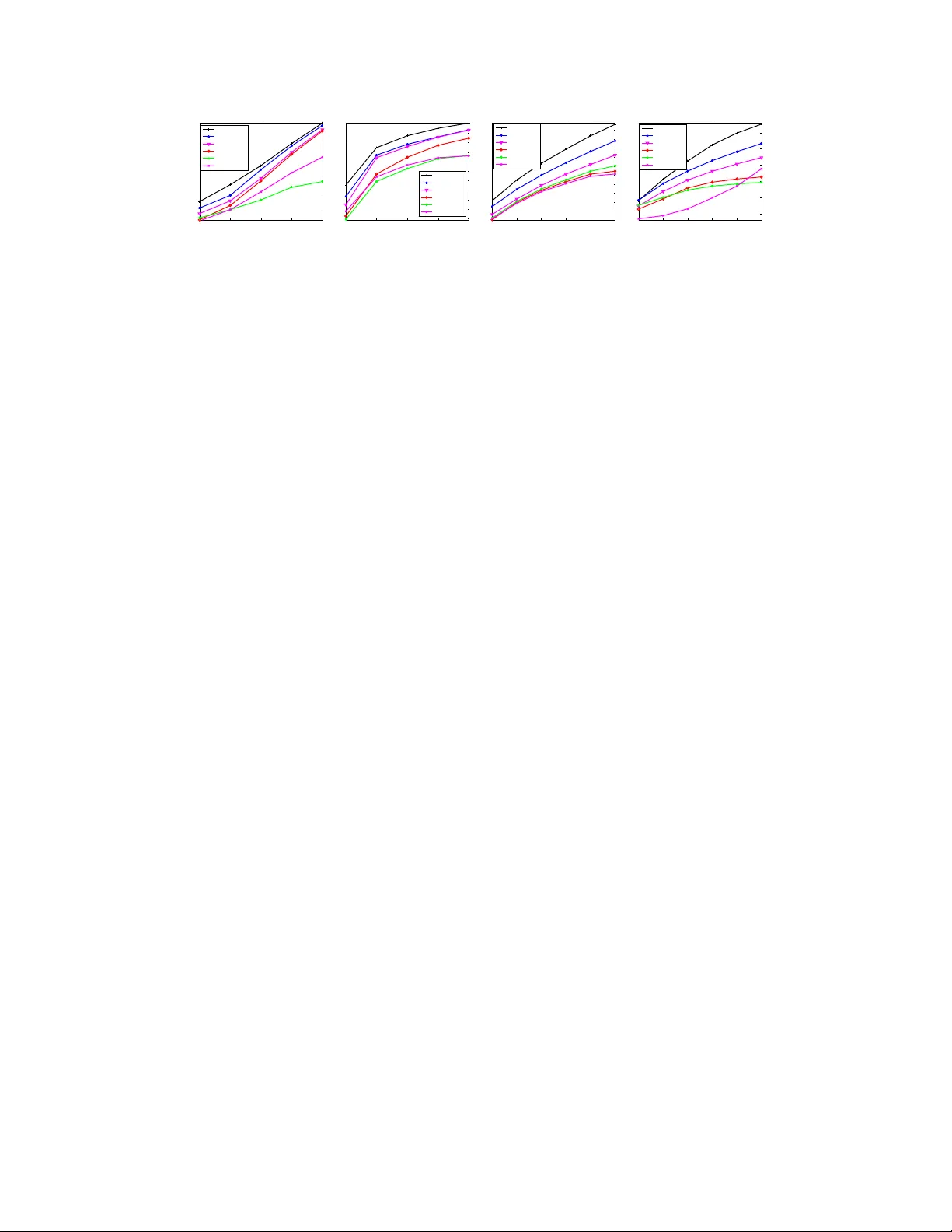
Authors: Hao Wang, Xingjian Shi, Dit-Yan Yeung
Collaborativ e Recurr ent A utoencoder: Recommend while Lear ning to Fill in the Blanks Hao W ang, Xingjian Shi, Dit-Y an Y eung Hong K ong Uni versity of Science and T echnology {hwangaz,xshiab,dyyeung}@cse.ust.hk Abstract Hybrid methods that utilize both content and rating information are commonly used in many recommender systems. Ho wev er , most of them use either handcrafted features or the bag-of-w ords representation as a surrog ate for the content infor - mation but the y are neither ef fectiv e nor natural enough. T o address this problem, we develop a collaborati ve recurrent autoencoder (CRAE) which is a denoising recurrent autoencoder (DRAE) that models the generation of content sequences in the collaborati ve filtering (CF) setting. The model generalizes recent adv ances in recurrent deep learning from i.i.d. input to non-i.i.d. (CF-based) input and pro vides a new denoising scheme along with a nov el learnable pooling scheme for the recur - rent autoencoder . T o do this, we first de velop a hierarchical Bayesian model for the DRAE and then generalize it to the CF setting. The synergy between denoising and CF enables CRAE to mak e accurate recommendations while learning to fill in the blanks in sequences. Experiments on real-world datasets from different domains (CiteULike and Netflix) sho w that, by jointly modeling the order-aware generation of sequences for the content information and performing CF for the ratings, CRAE is able to significantly outperform the state of the art on both the recommendation task based on ratings and the sequence generation task based on content information. 1 Introduction W ith the high pre v alence and ab undance of Internet services, recommender systems are becoming increasingly important to attract users because they can help users make ef fectiv e use of the informa- tion av ailable. Companies like Netflix ha ve been using recommender systems extensi vely to tar get users and promote products. Existing methods for recommender systems can be roughly cate gorized into three classes [ 13 ]: content-based methods that use the user profiles or product descriptions only , collaborativ e filtering (CF) based methods that use t he ratings only , and hybrid methods that make use of both. Hybrid methods using both types of information can get the best of both worlds and, as a result, usually outperform content-based and CF-based methods. Among the hybrid methods, collaborati v e topic regression (CTR) [ 21 ] was proposed to integrate a topic model and probabilistic matrix factorization (PMF) [ 15 ]. CTR is an appealing method in that it produces both promising and interpretable results. Howe v er , CTR uses a bag-of-words representation and ignores the order of words and the local context around each w ord, which can provide v aluable information when learning article representation and word embeddings. Deep learning models like con v olutional neural netw orks (CNN) which use layers of sliding windo ws (kernels) have the potential of capturing the order and local context of words. Ho wev er , the kernel size in a CNN is fixed during training. T o achiev e good enough performance, sometimes an ensemble of multiple CNNs with different kernel sizes has to be used. A more natural and adaptive w ay of modeling te xt sequences would be to use gated recurrent neural network (RNN) models [ 8 , 3 , 19 ]. A gated RNN takes in one 30th Conference on Neural Information Processing Systems (NIPS 2016), Barcelona, Spain. word (or multiple words) at a time and lets the learned gates decide whether to incorporate or to forget the word. Intuiti vely , if we can generalize gated RNNs to the CF setting (non-i.i.d.) to jointly model the generation of sequences and the relationship between items and users (rating matrices), the recommendation performance could be significantly boosted. Ne vertheless, v ery fe w attempts ha ve been made to dev elop feedforward deep learning models for CF , let alone recurrent ones. This is due partially to the fact that deep learning models, like many machine learning models, assume i.i.d. inputs. [ 16 , 6 , 7 ] use restricted Boltzmann machines and RNN instead of the con ventional matrix factorization (MF) formulation to perform CF . Although these methods in volv e both deep learning and CF , the y actually belong to CF-based methods because the y do not incorporate the content information lik e CTR, which is crucial for accurate recommendation. [ 14 ] uses low-rank MF in the last weight layer of a deep network to reduce the number of parameters, b ut it is for classification instead of recommendation tasks. There hav e also been nice e xplorations on music recommendation [ 10 , 26 ] in which a CNN or deep belief network (DBN) is directly used for content-based recommendation. Ho we ver , the models are deterministic and less robust since the noise is not explicitly modeled. Besides, the CNN is directly linked to the ratings making the performance suffer greatly when the ratings are sparse, as will be sho wn later in our experiments. V ery recently , collaborativ e deep learning (CDL) [ 24 ] is proposed as a probabilistic model for joint learning of a probabilistic stacked denoising autoencoder (SD AE) [ 20 ] and collaborati ve filtering. Howe v er , CDL is a feedforward model that uses bag-of-words as input and it does not model the order -aw are generation of sequences. Consequently , the model would hav e inferior r ecommendation performance and is not capable of gener ating sequences at all, which will be shown in our experiments. Besides order-a wareness, another drawback of CDL is its lack of r ob ustness (see Section 3.1 and 3.5 for details). T o address these problems, we propose a hierarchical Bayesian generativ e model called collaborati ve recurrent autoencoder (CRAE) to jointly model the order-a ware generation of sequences (in the content information) and the rating information in a CF setting. Our main contributions are: • By e xploiting recurrent deep learning collaborati vely , CRAE is able to sophisticatedly model the generation of items (sequences) while extracting the implicit relationship between items (and users). W e design a novel pooling scheme for pooling variable-length sequences into fixed-length vectors and also propose a ne w denoising scheme to effecti vely av oid overfitting. Besides for recommendation, CRAE can also be used to generate sequences on the fly . • T o the best of our kno wledge, CRAE is the first model that bridges the gap between RNN and CF , especially with respect to hybrid methods for recommender systems. Besides, the Bayesian nature also enables CRAE to seamlessly incorporate other auxiliary information to further boost the performance. • Extensiv e experiments on real-w orld datasets from different domains sho w that CRAE can substantially improv e on the state of the art. 2 Problem Statement and Notation Similar to [ 21 ], the recommendation task considered in this paper takes implicit feedback [ 9 ] as the training and test data. There are J items (e.g., articles or movies) in the dataset. For item j , there is a corresponding sequence consisting of T j words where the v ector e ( j ) t specifies the t -th w ord using the 1 -of- S representation, i.e., a vector of length S with the v alue 1 in only one element corresponding to the word and 0 in all other elements. Here S is the vocab ulary size of the dataset. W e define an I -by- J binary rating matrix R = [ R ij ] I × J where I denotes the number of users. F or example, in the CiteULike dataset, R ij = 1 if user i has article j in his or her personal library and R ij = 0 otherwise. Giv en some of the ratings in R and the corresponding sequences of words e ( j ) t (e.g., titles of articles or plots of movies), the problem is to predict the other ratings in R . In the follo wing sections, e 0 ( j ) t denotes the noise-corrupted version of e ( j ) t and ( h ( j ) t ; s ( j ) t ) refers to the concatenation of the two K W -dimensional column vectors. All input weights (like Y e and Y i e ) and recurrent weights (like W e and W i e ) are of dimensionality K W -by- K W . The output state h ( j ) t , gate units (e.g., h o t ( j ) ), and cell state s ( j ) t are of dimensionality K W . K is the dimensionality of the final representation γ j , middle-layer units θ j , and latent vectors v j and u i . I K or I K W denotes a K -by- K or K W -by- K W identity matrix. For con venience we use W + to denote the collection of all weights and biases. Similarly h + t is used to denote the collection of h t , h i t , h f t , and h o t . 2 h 1 h 1 h 2 h 2 h 3 h 3 h 4 h 4 h 5 h 5 s 1 s 1 s 2 s 2 s 3 s 3 s 4 s 4 s 5 s 5 e 0 1 e 0 1 e 0 2 e 0 2 e 1 e 1 e 2 e 2 µ µ ° ° v v J I R R u u ¸ u ¸ u ¸ v ¸ v J I E E E 0 E 0 ¸ w ¸ w W + W + v v R R u u ¸ u ¸ u µ µ A $ A B $ ¸ v ¸ v < ? > Figure 1: On the left is the graphical model for an example CRAE where T j = 2 for all j . T o pre vent clutter , the hyperparameters for beta-pooling, all weights, biases, and links between h t and γ are omitted. On the right is the graphical model for the degenerated CRAE. An example recurrent autoencoder with T j = 3 is sho wn. ‘ h ? i ’ is the h wildcard i and ‘$’ marks the end of a sentence. E 0 and E are used in place of [ e 0 ( j ) t ] T j t =1 and [ e ( j ) t ] T j t =1 respectiv ely . 3 Collaborative Recurr ent A utoencoder In this section we will first propose a generalization of the RNN called r obust r ecurr ent networks (RRN), follo wed by the introduction of two k ey concepts, wildcar d denoising and beta-pooling , in our model. After that, the generati ve process of CRAE is provided to show how to generalize the RRN as a hierarchical Bayesian model from an i.i.d. setting to a CF (non-i.i.d.) setting. 3.1 Robust Recurr ent Networks One problem with RNN models like long short-term memory networks (LSTM) is that the computa- tion is deterministic without taking the noise into account, which means it is not robust especially with insufficient training data. T o address this r ob ustness problem, we propose RRN as a type of noisy gated RNN. In RRN, the gates and other latent variables are designed to incorporate noise, making the model more robust. Note that unlike [ 4 , 5 ], the noise in RRN is directly propagated back and forth in the network, without the need for using separate neural networks to approximate the distributions of the latent variables. This is much more efficient and easier to implement. Here we provide the generati ve process of RRN. Using t = 1 . . . T j to index the w ords in the sequence, we hav e (we drop the index j for items for notational simplicity): x t − 1 ∼ N ( W w e t − 1 , λ − 1 s I K W ) , a t − 1 ∼ N ( Yx t − 1 + Wh t − 1 + b , λ − 1 s I K W ) (1) s t ∼ N ( σ ( h f t − 1 ) s t − 1 + σ ( h i t − 1 ) σ ( a t − 1 ) , λ − 1 s I K W ) , (2) where x t is the word embedding of the t -th word, W w is a K W -by- S word embedding matrix, e t is the 1 -of- S representation mentioned abov e, stands for the element-wise product operation between two vectors, σ ( · ) denotes the sigmoid function, s t is the cell state of the t -th word, and b , Y , and W denote the biases, input weights, and recurrent weights respecti vely . The forget gate units h f t and the input gate units h i t in Equation (2) are drawn from Gaussian distributions depending on their corresponding weights and biases Y f , W f , Y i , W i , b f , and b i : h f t ∼ N ( Y f x t + W f h t + b f , λ − 1 s I K W ) , h i t ∼ N ( Y i x t + W i h t + b i , λ − 1 s I K W ) . The output h t depends on the output gate h o t which has its own weights and biases Y o , W o , and b o : h o t ∼ N ( Y o x t + W o h t + b o , λ − 1 s I K W ) , h t ∼ N (tanh( s t ) σ ( h o t − 1 ) , λ − 1 s I K W ) . (3) In the RRN, information of the processed sequence is contained in the cell states s t and the output states h t , both of which are column vectors of length K W . Note that RRN can be seen as a generalized and Bayesian version of LSTM [ 1 ]. Similar to [ 19 , 3 ], two RRNs can be concatenated to form an encoder-decoder architecture. 3.2 Wildcard Denoising Since the input and output are identical here, unlike [ 19 , 3 ] where the input is from the source language and the output is from the tar get language, this naiv e RRN autoencoder can suf fer from serious ov erfitting, e ven after taking noise into account and reversing sequence order (we find that 3 rev ersing sequence order in the decoder [ 19 ] does not impro ve the recommendation performance). One natural way of handling it is to borro w ideas from the denoising autoencoder [ 20 ] by randomly dropping some of the words in the encoder . Unfortunately , directly dropping words may mislead the learning of transition between words. F or example, if we drop the word ‘is’ in the sentence ‘this is a good idea’, the encoder will wrongly learn the subsequence ‘this a’, which nev er appears in a grammatically correct sentence. Here we propose another denoising scheme, called wildcar d denoising , where a special word ‘ h wildcard i ’ is added to the v ocabulary and we randomly select some of the words and replace them with ‘ h wildcard i ’. This way , the encoder RRN will take ‘this h wildcard i a good idea’ as input and successfully a v oid learning wrong subsequences. W e call this denoising r ecurr ent autoencoder (DRAE). Note that the word ‘ h wildcard i ’ also has a corresponding word embedding. Intuitiv ely this wildcard denoising RRN autoencoder learns to fill in the blanks in sentences automatically . W e find this denoising scheme much better than the nai ve one. For example, in dataset CiteULike wildcard denoising can provide a relati v e accuracy boost of about 20% . 3.3 Beta-Pooling The RRN autoencoders would produce a representation vector for each input word. In order to facilitate the f actorization of the rating matrix, we need to pool the sequence of v ectors into one single v ector of fix ed length 2 K W before it is further encoded into a K -dimensional v ector . A natural way is to use a weighted average of the vectors. Unfortunately dif ferent sequences may need weights of differ ent size . F or example, pooling a sequence of 8 vectors needs a weight v ector with 8 entries while pooling a sequence of 50 vectors needs one with 50 entries. In other words, we need a weight vector of variable length for our pooling scheme. T o tackle this problem, we propose to use a beta distribution. If six vectors are to be pooled into one single vector (using weighted average), we can use the area w p in the range ( p − 1 6 , p 6 ) of the x -axis of the probability density function (PDF) for the beta distrib ution Beta ( a, b ) as the pooling weight. Then the resulting pooling weight v ector becomes y = ( w 1 , . . . , w 6 ) T . Since the total area is always 1 and the x -axis is bounded, the beta distribution is perfect for this type of variable-length pooling (hence the name beta-pooling ). If we set the hyperparameters a = b = 1 , it will be equi valent to a verage pooling. If a is set large enough and b > a the PDF will peak slightly to the left of x = 0 . 5 , which means that the last time step of the encoder RRN is directly used as the pooling result. W ith only two parameters, beta-pooling is able to pool vectors fle xibly enough without having the risk of o verfitting the data. 3.4 CRAE as a Hierarchical Bay esian Model Follo wing the notation in Section 2 and using the DRAE in Section 3.2 as a component, we then provide the generati ve process of the CRAE (note that t index es words or time steps, j index es sentences or documents, and T j is the number of words in document j ): Encoding ( t = 1 , 2 , . . . , T j ): Generate x 0 ( j ) t − 1 , a ( j ) t − 1 , and s ( j ) t according to Equation (1)-(2). Compression and decompr ession ( t = T j + 1 ): θ j ∼ N ( W 1 ( h ( j ) T j ; s ( j ) T j ) + b 1 , λ − 1 s I K ) , ( h ( j ) T j +1 ; s ( j ) T j +1 ) ∼ N ( W 2 tanh( θ j ) + b 2 , λ − 1 s I 2 K W ) . (4) Decoding ( t = T j + 2 , T j + 3 , . . . , 2 T j + 1 ): Generate a ( j ) t − 1 , s ( j ) t , and h ( j ) t according to Equa- tion (1)-(3), after which generate: e ( j ) t − T j − 2 ∼ Mult ( softmax ( W g h ( j ) t + b g )) . Beta-pooling and recommendation : γ j ∼ N (tanh( W 1 f a,b ( { ( h ( j ) t ; s ( j ) t ) } t ) + b 1 ) , λ − 1 s I K ) (5) v j ∼ N ( γ j , λ − 1 v I K ) , u i ∼ N ( 0 , λ − 1 u I K ) , R ij ∼ N ( u T i v j , C − 1 ij ) . Note that each column of the weights and biases in W + is drawn from N ( 0 , λ − 1 w I K W ) or N ( 0 , λ − 1 w I K ) . In the generati ve process above, the input gate h i t − 1 ( j ) and the for get gate h f t − 1 ( j ) can be dra wn as described in Section 3.1. e 0 ( j ) t denotes the corrupted word (with the embedding 4 x 0 ( j ) t ) and e ( j ) t denotes the original word (with the embedding x ( j ) t ). λ w , λ u , λ s , and λ v are hy- perparameters and C ij is a confidence parameter ( C ij = α if R ij = 1 and C ij = β otherwise). Note that if λ s goes to infinity , the Gaussian distribution (e.g., in Equation (4)) will become a Dirac delta distribution centered at the mean. The compression and decompression act like a bottleneck between two Bayesian RRNs. The purpose is to reduce overfitting, provide necessary nonlinear transformation, and perform dimensionality reduction to obtain a more compact final representa- tion γ j for CF . The graphical model for an example CRAE where T j = 2 for all j is shown in Figure 1(left). f a,b ( { ( h ( j ) t ; s ( j ) t ) } t ) in Equation (5) is the result of beta-pooling with hyperparameters a and b . If we denote the cumulativ e distribution function of the beta distribution as F ( x ; a, b ) , φ ( j ) t = ( h ( j ) t ; s ( j ) t ) for t = 1 , . . . , T j , and φ ( j ) t = ( h ( j ) t +1 ; s ( j ) t +1 ) for t = T j + 1 , . . . , 2 T j , then we hav e f a,b ( { ( h ( j ) t ; s ( j ) t ) } t ) = P 2 T j t =1 ( F ( t 2 T j , a, b ) − F ( t − 1 2 T j , a, b )) φ t . Please see Section C of the supplementary materials for details (including hyperparameter learning) of beta-pooling. From the generativ e process, we can see that both CRAE and CDL are Bayesian deep learning (BDL) models (as described in [ 25 ]) with a perception component (DRAE in CRAE) and a task-specific component. 3.5 Learning According to the CRAE model above, all parameters like h ( j ) t and v j can be treated as random variables so that a full Bayesian treatment such as methods based on variational approximation can be used. Howe ver , due to the extreme nonlinearity and the CF setting, this kind of treatment is non-trivial. Besides, with CDL [ 24 ] and CTR [ 21 ] as our primary baselines, it would be fairer to use maximum a posteriori (MAP) estimates, which is what CDL and CTR do. End-to-end joint learning : Maximization of the posterior probability is equi v alent to maximizing the joint log-likelihood of { u i } , { v j } , W + , { θ j } , { γ j } , { e ( j ) t } , { e 0 ( j ) t } , { h + t ( j ) } , { s ( j ) t } , and R giv en λ u , λ v , λ w , and λ s : L = log p ( DRAE | λ s , λ w ) − λ u 2 X i k u i k 2 2 − λ v 2 X j k v j − γ j k 2 2 − X i,j C ij 2 ( R ij − u T i v j ) 2 − λ s 2 X j k tanh( W 1 f a,b ( { ( h ( j ) t ; s ( j ) t ) } t ) + b 1 ) − γ j k 2 2 , where log p ( DRAE | λ s , λ w ) corresponds to the prior and likelihood terms for DRAE (including the encoding, compression, decompression, and decoding in Section 3.4) in volving W + , { θ j } , { e ( j ) t } , { e 0 ( j ) t } , { h + t ( j ) } , and { s ( j ) t } . For simplicity and computational efficiency , we can fix the hyperparameters of beta-pooling so that Beta ( a, b ) peaks slightly to the left of x = 0 . 5 (e.g., a = 9 . 8 × 10 7 , b = 1 × 10 8 ), which leads to γ j = tanh( θ j ) (a treatment for the more general case with learnable a or b is provided in the supplementary materials). Further , if λ s approaches infinity , the terms with λ s in log p ( DRAE | λ s , λ w ) will vanish and γ j will become tanh( W 1 ( h ( j ) T j , s ( j ) T j ) + b 1 ) . Figure 1(right) sho ws the graphical model of a degenerated CRAE when λ s approaches positi ve infinity and b > a (with very large a and b ). Learning this degenerated version of CRAE is equi v alent to jointly training a wildcard denoising RRN and an encoding RRN coupled with the rating matrix. If λ v 1 , CRAE will further degenerate to a two-step model where the representation θ j learned by the DRAE is directly used for CF . On the contrary if λ v 1 , the decoder RRN essentially vanishes. Both extreme cases can greatly de grade the predictiv e performance, as sho wn in the experiments. Robust nonlinearity on distributions : Different from [ 24 , 23 ], nonlinear transformation is per- formed after adding the noise with precision λ s (e.g. a ( j ) t in Equation (1)). In this case, the input of the nonlinear transformation is a distribution rather than a deterministic value , making the nonlinearity more robust than in [24, 23] and leading to more ef ficient and direct learning algorithms than CDL. Consider a univ ariate Gaussian distrib ution N ( x | µ, λ − 1 s ) and the sigmoid function σ ( x ) = 1 1+exp( − x ) , the expectation (see Section F of the supplementary materials for details): E ( x ) = Z N ( x | µ, λ − 1 s ) σ ( x ) dx = σ ( κ ( λ s ) µ ) , (6) Equation (9) holds because the conv olution of a sigmoid function with a Gaussian distrib ution can be approximated by another sigmoid function. Similarly , we can approximate σ ( x ) 2 with σ ( ρ 1 ( x + ρ 0 )) , 5 where ρ 1 = 4 − 2 √ 2 and ρ 0 = − log( √ 2 + 1) . Hence the variance D ( x ) ≈ Z N ( x | µ, λ − 1 s ) ◦ Φ( ξ ρ 1 ( x + ρ 0 )) dx − E ( x ) 2 = σ ( ρ 1 ( µ + ρ 0 ) (1 + ξ 2 ρ 2 1 λ − 1 s ) 1 / 2 ) − E ( x ) 2 ≈ λ − 1 s , (7) where we use λ − 1 s to approximate D ( x ) for computational ef ficiency . Using Equation (9) and (10), the Gaussian distribution in Equation (2) can be computed as: N ( σ ( h f t − 1 ) s t − 1 + σ ( h i t − 1 ) σ ( a t − 1 ) , λ − 1 s I K W ) ≈ N ( σ ( κ ( λ s ) h f t − 1 ) s t − 1 + σ ( κ ( λ s ) h i t − 1 ) σ ( κ ( λ s ) a t − 1 ) , λ − 1 s I K W ) , (8) where the superscript ( j ) is dropped. W e use ov erlines (e.g., a t − 1 = Y e x t − 1 + W e h t − 1 + b e ) to denote the mean of the distrib ution from which a hidden variable is drawn. By applying Equation (11) recursiv ely , we can compute s t for any t . Similar approximation is used for tanh( x ) in Equation (3) since tanh( x ) = 2 σ (2 x ) − 1 . This way the feedforward computation of DRAE w ould be seamlessly chained together , leading to more efficient learning algorithms than the layer-wise algorithms in [24, 23] (see Section F of the supplementary materials for more details). Learning parameters : T o learn u i and v j , block coordinate ascent can be used. Gi ven the current W + , we can compute γ as γ = tanh( W 1 f a,b ( { ( h ( j ) t ; s ( j ) t ) } t ) + b 1 ) and get the follo wing update rules: u i ← ( V C i V T + λ u I K ) − 1 V C i R i v j ← ( UC i U T + λ v I K ) − 1 ( UC j R j + λ v tanh( W 1 f a,b ( { ( h ( j ) t ; s ( j ) t ) } t ) + b 1 ) T ) , where U = ( u i ) I i =1 , V = ( v j ) J j =1 , C i = diag ( C i 1 , . . . , C iJ ) is a diagonal matrix, and R i = ( R i 1 , . . . , R iJ ) T is a column vector containing all the ratings of user i . Giv en U and V , W + can be learned using the back-propagation algorithm according to Equation (9)-(11) and the generativ e process in Section 3.4. Alternating the update of U , V , and W + giv es a local optimum of L . After U and V are learned, we can predict the ratings as R ij = u T i v j . 4 Experiments In this section, we report some experiments on real-world datasets from dif ferent domains to ev aluate the capabilities of recommendation and automatic generation of missing sequences. 4.1 Datasets W e use two datasets from different real-w orld domains. CiteULike is from [ 21 ] with 5 , 551 users and 16 , 980 items (articles with text). Netflix consists of 407 , 261 users, 9 , 228 movies, and 15 , 348 , 808 ratings after removing users with less than 3 positiv e ratings (following [ 24 ], ratings larger than 3 are regarded as positi v e ratings). Please see Section G of the supplementary materials for details. 4.2 Evaluation Schemes Recommendation : For the recommendation task, similar to [ 22 , 24 ], P items associated with each user are randomly selected to form the training set and the rest is used as the test set. W e ev aluate the models when the ratings are in different degrees of density ( P ∈ { 1 , 2 , . . . , 5 } ). For each value of P , we repeat the ev aluation fi ve times with dif ferent training sets and report the a verage performance. Follo wing [ 21 , 22 ], we use recall as the performance measure since the ratings are in the form of implicit feedback [ 9 , 12 ]. Specifically , a zero entry may be due to the fact that the user is not interested in the item, or that the user is not a ware of its existence. Thus precision is not a suitable performance measure. W e sort the predicted ratings of the candidate items and recommend the top M items for the target user . The recall@ M for each user is then defined as: recall@ M = # items that the user likes among the top M # items that the user likes . The av erage recall ov er all users is reported. 6 1 2 3 4 5 0.1 0.15 0.2 0.25 0.3 0.35 P Recall CRAE CDL CTR DeepMusic CMF SVDFeature 1 2 3 4 5 0.15 0.2 0.25 0.3 0.35 0.4 0.45 0.5 0.55 0.6 0.65 P Recall CRAE CDL CTR DeepMusic CMF SVDFeature 50 100 150 200 250 300 0.02 0.03 0.04 0.05 0.06 0.07 0.08 0.09 0.1 0.11 0.12 M Recall CRAE CDL CTR DeepMusic CMF SVDFeature 50 100 150 200 250 300 0.05 0.1 0.15 0.2 0.25 0.3 M Recall CRAE CDL CTR DeepMusic CMF SVDFeature Figure 2: Performance comparison of CRAE, CDL, CTR, DeepMusic, CMF , and SVDFeature based on recall@ M for datasets CiteULike and Netflix . P is v aried from 1 to 5 in the first two figures. W e also use another e valuation metric, mean a verage precision (mAP), in the experiments. Exactly the same as [10], the cutoff point is set at 500 for each user . Sequence generation on the fly : For the sequence generation task, we set P = 5 . In terms of content information (e.g., movie plots), we randomly select 80% of the items to include their content in the training set. The trained models are then used to predict (generate) the content sequences for the other 20% items. The BLEU score [ 11 ] is used to ev aluate the quality of generation. T o compute the BLEU score in CiteULike we use the titles as training sentences (sequences). Both the titles and sentences in the abstracts of the articles (items) are used as reference sentences. For Netflix , the first sentences of the plots are used as training sentences. The movie names and sentences in the plots are used as reference sentences. A higher BLEU score indicates higher quality of sequence generation. Since CDL, CTR, and PMF cannot g enerate sequences dir ectly , a nearest neighborhood based approach is used with the resulting v j . Note that this task is e xtremely dif ficult because the sequences of the test set are unknown during both the training and testing phases . F or this reason, this task is impossible for existing machine translation models like [19, 3]. 4.3 Baselines and Experimental Settings The models for comparison are listed as follows: • CMF : Collective Matrix Factorization [ 17 ] is a model incorporating different sources of information by simultaneously factorizing multiple matrices. • SVDFeatur e : SVDFeature [ 2 ] is a model for feature-based collaborative filtering. In this paper we use the bag-of-words as raw features to feed into SVDFeature. • DeepMusic : DeepMusic [ 10 ] is a feedforward model for music recommendation mentioned in Section 1. W e use the best performing variant as our baseline. • CTR : Collaborati ve T opic Regression [ 21 ] is a model performing topic modeling and collaborativ e filtering simultaneously as mentioned in the pre vious section. • CDL : Collaborativ e Deep Learning (CDL) [ 24 ] is proposed as a probabilistic feedforward model for joint learning of a probabilistic SD AE [20] and CF . • CRAE : Collaborati ve Recurrent Autoencoder is our proposed r ecurr ent model. It jointly performs collaborativ e filtering and learns the generation of content (sequences). In the experiments, we use 5-fold cross validation to find the optimal hyperparameters for CRAE and the baselines. For CRAE, we set α = 1 , β = 0 . 01 , K = 50 , K W = 100 . The wildcard denoising rate is set to 0 . 4 . See Section E.1 of the supplementary materials for details. 4.4 Quantitative Comparison Recommendation : The first two plots of Figure 2 show the recall@ M for the two datasets when P is varied from 1 to 5 . As we can see, CTR outperforms the other baselines except for CDL. Note that as previously mentioned, in both datasets DeepMusic suf fers badly from ov erfitting when the rating matrix is extremely sparse ( P = 1 ) and achiev es comparable performance with CTR when the rating matrix is dense ( P = 5 ). CDL as the strongest baseline consistently outperforms other baselines. By jointly learning the order -aware generation of content (sequences) and performing collaborativ e filtering, CRAE is able to outperform all the baselines by a margin of 0 . 7% ∼ 1 . 9% (a relativ e boost of 2 . 0% ∼ 16 . 7% ) in CiteULike and 3 . 5% ∼ 6 . 0% (a relative boost of 5 . 7% ∼ 22 . 5% ) in Netflix . Note that since the standard deviation is minimal ( 3 . 38 × 10 − 5 ∼ 2 . 56 × 10 − 3 ), it is not included in the figures and tables to av oid clutter . The last two plots of Figure 2 show the recall@ M for CiteULike and Netflix when M varies from 50 to 300 and P = 1 . As shown in the plots, the performance of DeepMusic, CMF , and SVDFeature is 7 0 0.5 1 0 50 100 150 200 250 (a) 0 0.5 1 0 5 10 15 20 25 (b) 0 0.5 1 0 2 4 6 8 10 (c) 0 0.5 1 0 0.5 1 1.5 2 (d) 0 0.5 1 0 5 10 15 (e) 0 0.5 1 0 2 4 6 8 10 (f) 0 0.5 1 0 5 10 15 20 25 (g) 0 0.5 1 0 50 100 150 200 250 (h) Figure 3: The shape of the beta distribution for dif ferent a and b (corresponding to T able 5). T able 1: Recall@300 for beta-pooling with different hyperparameters a 31112 311 1 1 0.4 10 400 40000 b 40000 400 10 1 0.4 1 311 31112 Recall 12.17 12.54 10.48 11.62 11.08 10.72 12.71 12.22 T able 2: mAP for two datasets CRAE CDL CTR DeepMusic CMF SVDFeature CiteULike 0.0123 0.0091 0.0071 0.0058 0.0061 0.0056 Netflix 0.0301 0.0275 0.0211 0.0156 0.0144 0.0173 T able 3: BLEU score for two datasets CRAE CDL CTR PMF CiteULike 46.60 21.14 31.47 17.85 Netflix 48.69 6.90 17.17 11.74 similar in this setting. Again CRAE is able to outperform the baselines by a large margin and the margin gets lar ger with the increase of M . As sho wn in Figure 4 and T able 5, we also in vestigate the ef fect of a and b in beta-pooling and find that in DRAE: (1) temporal a verage pooling performs poorly ( a = b = 1 ); (2) most information concentrates near the bottleneck; (3) the right of the bottleneck contains more information than the left. Please see Section D of the supplementary materials for more details. As another ev aluation metric, T able 2 compares dif ferent models based on mAP . As we can see, compared with CDL, CRAE can provide a relative boost of 35% and 10% for CiteULike and Netflix , respecti vely . Besides quantitativ e comparison, qualitative comparison of CRAE and CDL is provided in Section B of the supplementary materials. In terms of time cost, CDL needs 200 epochs ( 40 s/epoch) while CRAE needs about 80 epochs ( 150 s/epoch) for optimal performance. Sequence generation on the fly : T o e valuate the ability of sequence generation, we compute the BLEU score of the sequences (titles for CiteULike and plots for Netflix ) generated by dif ferent models. As mentioned in Section 4.2, this task is impossible for e xisting machine translation models like [ 19 , 3 ] due to the lack of source sequences. As we can see in T able 3, CRAE achiev es a BLEU score of 46 . 60 for CiteULike and 48 . 69 for Netflix , which is much higher than CDL, CTR and PMF . Incorporating the content information when learning user and item latent v ectors, CTR is able to outperform other baselines and CRAE can further boost the BLEU score by sophisticatedly and jointly modeling the generation of sequences and ratings. Note that although CDL is able to outperform other baselines in the recommendation task, it performs poorly when generating sequences on the fly , which demonstrates the importance of modeling each sequence recurrently as a whole rather than as separate words. 5 Conclusions and Future W ork W e dev elop a collaborativ e recurrent autoencoder which can sophisticatedly model the generation of item sequences while extracting the implicit relationship between items (and users). W e design a new pooling scheme for pooling v ariable-length sequences and propose a wildcard denoising scheme to effecti v ely avoid ov erfitting. T o the best of our kno wledge, CRAE is the first model to bridge the gap between RNN and CF . Extensiv e experiments sho w that CRAE can significantly outperform the state-of-the-art methods on both the recommendation and sequence generation tasks. W ith its Bayesian nature, CRAE can easily be generalized to seamlessly incorporate auxiliary information (e.g., the citation network for CiteULike and the co-director network for Netflix ) for further accurac y boost. Moreover , multiple Bayesian recurrent layers may be stacked together to increase its representation power . Besides making recommendations and guessing sequences on the fly , the wildcard denoising recurrent autoencoder also has potential to solve other challenging problems such as recov ering the blurred words in ancient documents. 8 A Learning Beta-P ooling As mentioned in the paper , f a,b ( { ( h ( j ) t ; s ( j ) t ) } t ) is the result of beta-pooling. The cumulati v e distribution function of the beta distribution F ( x ; a, b ) = B ( x ; a,b ) B ( a,b ) = I x ( a, b ) , where B ( x ; a, b ) = R x 0 t a − 1 (1 − t ) b − 1 dt is the incomplete beta function and the denominator B ( a, b ) = Γ( a + b ) Γ( a ) Γ( b ) . Γ( · ) is the gamma function and I x ( a, b ) is also called the re gularized incomplete beta function. If we denote φ ( j ) t = ( h ( j ) t ; s ( j ) t ) for t = 1 , . . . , T j and φ ( j ) t = ( h ( j ) t +1 ; s ( j ) t +1 ) for t = T j + 1 , . . . , 2 T j , we hav e f a,b ( { ( h ( j ) t ; s ( j ) t ) } t ) = 2 T j P t =1 ( I t 2 T j ( a, b ) − I t − 1 2 T j ( a, b )) φ t . Written this way , we can e v aluate the gradient of L with respect to a and b and use gradient-based methods to learn them. T o illustrate it more clearly , if we take λ s to positi ve infinity , fix b = 1 and try to learn the optimal value of a , we can maximize the following joint log-lik elihood: L = − X i,j C ij 2 ( R ij − u T i v j ) 2 − λ v 2 X j k v j − tanh( W 1 2 T j X t =1 [ I t 2 T j ( a, 1) − I t − 1 2 T j ( a, 1)] φ t + b 1 ) k 2 2 + X j 2 T j +1 X t = T j +2 H ( e ( j ) t − T j − 1 , softmax ( W g h ( j ) t + b g )) − λ u 2 X i k u i k 2 2 − λ w 2 g ( W + ) . Note that H ( · , · ) denotes the cross-entropy loss for generating words from Mult ( softmax ( W g h ( j ) t + b g )) . The term − λ w 2 g ( W + ) corresponds to the prior of all weights and biases. Using the property of the regularized incomplete beta function that I x ( a, 1) = x a , the joint log-lik elihood can be simplified to L = − λ v 2 X j k v j − tanh( W 1 2 T j X t =1 [( t 2 T j ) a − ( t − 1 2 T j ) a ] φ t + b 1 ) k 2 2 − λ u 2 X i k u i k 2 2 − X i,j C ij 2 ( R ij − u T i v j ) 2 + X j 2 T j +1 X t = T j +2 H ( e ( j ) t − T j − 1 , softmax ( W g h ( j ) t + b g )) − λ w 2 g ( W + ) , where a only appears in the e xponents of ( t 2 T j ) a and ( t − 1 2 T j ) a , which means we can easily get the gradient of L with respect to a using the chain rule. After each epoch or minibatch, a can be updated based on the gradient with the same learning rate. B Qualitative Comparison In order to gain a better insight into CRAE, we train CRAE and CDL in the sparsest setting ( P = 1 ) with dataset CiteULike and use them to recommend articles for two example users. The corresponding articles for the target users in the training set and the top 10 recommended articles are sho wn in T able 4. Note that in the sparsest setting the recommendation task is extremely challenging since there is only one single article for each user in the training set. As we can see, CRAE successfully identified User I as a researcher working on information retrieval with interest in user modeling using user feedback . Consequently , CRAE achiev es a high precision of 60% by focusing its recommendations on articles about information retriev al, user modeling, and rele vance feedback. On the other hand, the topics of articles recommended by CDL span from visual tracking (Article 4 ) to bioinformatics (Article 3 ) and programming language (Article 8 ). One possible reason is that CDL uses the bag-of-words representation as input and consider each word separately without taking into account the local context of w ords. For example, looking into CDL ’ s recommendations more closely , we can find that Article 3 (on bioinformatics) and Article 4 (on visual tracking) are actually irrele vant to the training article ‘ Bayesian adaptiv e user profiling with explicit and implicit feedback’. CDL probably recommends Article 3 because the w ord ‘ profiles ’ in the title ov erlaps with the article in the training set. The same thing happens for Article 4 with a word ‘ Bayesian ’. W ith the recurrent learning in CRAE, a sequence is modeled as a whole instead of separate words. As a result, with the local context of each word taken into consideration, CRAE can recognize the whole phrase ‘ user pr ofiling ’, rather than ‘user’ or ‘profiling’, as a theme of the article. 9 T able 4: Qualitative comparison between CRAE and CDL the rated article Bayesian adaptiv e user profiling with explicit and implicit feedback User I (CRAE) in user’ s lib? top 10 articles 1. Incorporating user search behavior into relev ance feedback no 2. Query chains: lear ning to rank from implicit feedback yes 3. Implicit feedback for inferring user prefer ence: a bibliograph y yes 4. Modeling user rating profiles for collaborative filtering no 5. Improving retriev al performance by relev ance feedback no 6. Language models for relevance feedback no 7. Context-sensitive information r etrieval using implicit feedback yes 8. Implicit user modeling for personalized search yes 9. Model-based feedback in the language modeling approach to information r etrieval yes 10. User language model for collaborative personalized sear ch yes User I (CDL) in user’ s lib? top 10 articles 1. Implicit feedback for inferring user prefer ence: a bibliograph y yes 2. Seeing stars: Exploiting class relationships for sentiment cate gorization with respect to rating scales no 3. A knowledge-based approach for interpreting genome-wide expression profiles no 4. A tutorial on particle filters for online non-linear/non-gaussian Bayesian tracking no 5. Query chains: lear ning to rank from implicit feedback yes 6. Mapreduce: simplified data processing on lar ge clusters no 7. Correlating user profiles from multiple folksonomies no 8. Evolving object-oriented designs with refactorings no 9. Trapping of neutral sodium atoms with radiation pressure no 10. A scheme for efficient quantum computation with linear optics no the rated article T axonomy of trust: categorizing P2P reputation systems User II (CRAE) in user’ s lib? top 10 articles 1. Effects of positiv e reputation systems no 2. T rust in recommender systems yes 3. trust metrics in recommender systems no 4. The Structure of Collaborative T agging Systems no 5. Effects of energy policies on industry expansion in rene wable ener gy no 6. Limited reputation sharing in P2P systems yes 7. Survey of wireless indoor positioning techniques and systems no 8. Design coordination in distributed environments using virtual reality systems no 9. Propagation of trust and distrust yes 10. Physiological measures of presence in stressful virtual environments no User II (CDL) in user’ s lib? top 10 articles 1. T rust in recommender systems yes 2. Position Paper, T agging, T axonomy , Flickr, Article, T oRead no 3. A taxonomy of workflow management systems for grid computing no 4. Usage patterns of collaborative tagging systems no 5. Semantic blogging and decentralized knowledge management no 6. Flickr tag recommendation based on collective kno wledge no 7. Delivering real-world ubiquitous location systems no 8. Shilling recommender systems for fun and profit no 9. Privac y risks in recommender systems no 10. Probabilistic reasoning in intelligent systems networks of plausible inference no A similar phenomenon is found for User II with the article ‘T axonomy of trust: categorizing P2P reputation systems ’. CDL ’ s recommendations bet on the single word ‘systems’ while CRAE identified the article to be on trust pr opagation from the words ‘trust’ and ‘P2P’. In the end, CRAE achiev es a precision of 30% and CDL ’ s precision is 10% . C Motivation of Beta-P ooling The function f a,b ( { ( h ( j ) t ; s ( j ) t ) } t ) is to pool the output states h ( j ) t and the cell states s ( j ) t of 2 T j steps (a 2 K W -by- 2 T j matrix) into a single vector of length 2 K W . If we denote the cumulati ve distribution function of the beta distrib ution as F ( x ; a, b ) , φ ( j ) t = ( h ( j ) t ; s ( j ) t ) for t = 1 , . . . , T j , and φ ( j ) t = ( h ( j ) t +1 ; s ( j ) t +1 ) for t = T j + 1 , . . . , 2 T j , then we hav e f a,b ( { ( h ( j ) t ; s ( j ) t ) } t ) = 2 T j X t =1 ( F ( t 2 T j , a, b ) − F ( t − 1 2 T j , a, b )) φ t . Note that a and b are hyperparameters here. In a generalized setting, the y can be learned automatically . Essentially the motivation of beta-pooling is to handle the variable length for differ ent sequences using one unified distribution . When a = 2 and b = 3 , the beta-pooling is close to av erage pooling but with lar ger weights to the left of the center (the bottleneck). F ollo wing the generativ e process, the output h ( j ) t and cell states 10 0 0.5 1 0 50 100 150 200 250 (a) 0 0.5 1 0 5 10 15 20 25 (b) 0 0.5 1 0 2 4 6 8 10 (c) 0 0.5 1 0 0.5 1 1.5 2 (d) 0 0.5 1 0 5 10 15 (e) 0 0.5 1 0 2 4 6 8 10 (f) 0 0.5 1 0 5 10 15 20 25 (g) 0 0.5 1 0 50 100 150 200 250 (h) Figure 4: The shape of the beta distribution for dif ferent a and b (corresponding to T able 5). T able 5: Recall@300 for beta-pooling with different hyperparameters a 31112 311 1 1 0.4 10 400 40000 b 40000 400 10 1 0.4 1 311 31112 Recall 12.17 12.54 10.48 11.62 11.08 10.72 12.71 12.22 s ( j ) t of each word are concatenated into ( h ( j ) t ; s ( j ) t ) . For each sequence, ( h ( j ) t ; s ( j ) t ) of all timesteps are beta-pooled into a vector of length 2 K W . The vector is then further encoded into the vector γ j of length K , which is used to guide the CF for the rating matrix. Since the information flo ws in both ways, the rating matrix can, in return, provide useful information when the wildcard denoising recurrent autoencoder tries to learn to fill in the blanks. This two-way interaction enables both tasks (recommendation task and sequence generation task) to benefit from each other and results in more effecti v e representation θ j for each item. Note that the compression layer and the beta-pooling share the same weights and biases. If the hyperparameters of beta-pooling are fixed so that Beta ( a, b ) peaks slightly to the left of x = 0 . 5 , the generation of γ j in the generati ve process is equi valent to directly setting γ j = tanh( θ j ) where θ j is the compressed representation we get from the compression layer . For e xample, Beta ( a, b ) peaks slightly to the left of x = 0 . 5 (near x = 7 16 ) when a = 7778 , b = 10000 , and T j = 4 . The only time step that interacts with the rating matrix is the one when t = 4 , which is encoded into θ j and connected to the item latent vector v j . D Experiments on Beta-Pooling and W ildcard Denoising As mentioned in the paper , beta-pooling is able to pool a sequence of 2 T j vectors into one single vector of the same size. Note that T j here can v ary for different j . Hyperparameters a and b control the behavior of beta-pooling. When a = b = 1 , beta-pooling is equivalent to temporal average pooling that takes the av erage of the 2 T j vectors. In an extreme case, a and b can be set such that the pooling result is equal to one of the 2 T j vectors (e.g., the T j -th vector). Figure 4 shows the shape of the beta distribution for different a and b . T able 5 sho ws the corresponding recall for different beta distributions in CiteULike . As we can see, the a verage pooling in Figure 4(d) and the pooling with an in verted bell curv e in Figure 4(e) perform poorly . On the other hand, distributions in Figure 4(a), (b), (g), and (h) yield the highest accurac y , which means most information concentrates near the bottleneck (middle) of DRAE. Among them, the distributions in Figure 4(b) and (g) outperform those in Figure 4(a) and (h). This shows that simply setting the pooling result to be the middle v ector is not good enough and an aggreg ation of v ectors near the middle would be a better choice. Comparing distributions in Figure 4(b) and (g), it can be seen that the latter slightly outperforms the former , probably because there are no input words in the decoder part of DRAE (as shown in the graphical model of CRAE), which makes the hidden and cell states in the decoder part more representativ e. Similar phenomena happen for Figure 4(a), (c), (f), and (h). Note that since CRAE is a joint model, the information flo ws both w ays through beta-pooling. For example, when a = 400 and b = 311 , the item representations used for recommendation mostly come from the cell and output states near the bottleneck and in return, the rating information affects the learning of DRAE mainly through the cell and output states near the bottleneck. As mentioned in the paper , for the wildcard denoising scheme, we find that in CiteULike , CRAE performs best with a wildcard denoising rate of 0 . 4 , achieving a recall@300 of 12 . 71% while the number for CRAE with conv entional denoising [ 20 ] (dropping words completely) is 10 . 53% (slightly better than CDL). For reference, the recall of CRAE without any denoising is 9 . 14% . Similar phenomena are found in Netflix . 11 10 −3 10 −2 10 −1 10 0 10 1 0.05 0.1 0.15 0.2 0.25 0.3 0.35 λ v Recall M=300 M=200 M=100 Figure 5: The recall@ M for different λ v . Note that DRAE is a much more general model than RNN autoencoders like [ 19 , 18 ]. W e also try rev ersing the order of each sequence in the decoder RNN as in [ 19 , 18 ], but the performance only changes slightly . E Hyperparameters W e provide more details on the hyperparameters in this section. E.1 Hyperparameter Settings The vocab ulary size S (with the word h w ildcar d i included) is 15 , 050 and 17 , 949 for CiteULike and Netflix respecti vely . F or CMF and SVDFeature, optimal regularization hyperparameters are used for dif ferent P . The learning rate is set to 0 . 005 for SVDFeature. For DeepMusic, we find that the best performance is achie v ed using a CNN with two con volutional layers. F or CTR, we find that it can achieve good prediction performance when λ u = 0 . 1 , λ v = 10 , and K = 50 . For CDL, we use similar hyperparameters as mentioned in [ 24 ]. The denoising rate is set to 0 . 3 . Dropout rate, λ u , λ v , and λ n are set using the v alidation sets. For the sequence generation task, we postprocess the generated sequences by deleting consecuti ve repeated words (e.g., the word ‘like’ in the sentence ‘I like like this idea’), as often done in RNN-based sentence generation models. E.2 Hyperparameter Sensitivity Figure 5 shows the recall@ M for CiteULike when λ v is from 0 . 001 to 10 ( P = 5 ). As mentioned in the paper , when λ v 1 CRAE degenerates to a tw o-step model with no joint learning on the content sequences and ratings. If λ v 1 the decoder side of CRAE will essentially vanish. Apparently the performance suffers a lot in both extremes, which sho ws the effecti veness of joint learning in the full CRAE model. F Robust Nonlinearity on Distrib utions Different from [24], nonlinear transformation is performed after adding the noise with precision λ s . In this case, the input of the nonlinear transformation is a distribution rather than a deterministic value , making the nonlinearity more robust than in [ 24 ] and leading to more ef ficient and direct learning algorithms than CDL. Consider a univ ariate Gaussian distrib ution N ( x | µ, λ − 1 s ) and the sigmoid function σ ( x ) = 1 1+exp( − x ) , the expectation: E ( x ) = Z N ( x | µ, λ − 1 s ) σ ( x ) dx ≈ Z N ( x | µ, λ − 1 s )Φ( ξ x ) dx = Φ( ξ κ ( λ s ) µ ) = σ ( κ ( λ s ) µ ) , (9) where the probit function Φ( x ) = R x −∞ N ( θ | 0 , 1) dθ , κ ( λ s ) = (1 + ξ 2 λ − 1 s ) − 1 2 , and Φ( ξ x ) , with ξ 2 = π 8 , is to approximate σ ( x ) by matching the slope at the origin. Equation (9) holds because the 12 con v olution of a probit function with a Gaussian distribution is another probit function. Similarly , we can approximate σ ( x ) 2 with σ ( ρ 1 ( x + ρ 0 )) by matching both the v alue and the slope at the origin, where ρ 1 = 4 − 2 √ 2 and ρ 0 = − log( √ 2 + 1) . Hence the variance D ( x ) ≈ Z N ( x | µ, λ − 1 s ) ◦ Φ( ξ ρ 1 ( x + ρ 0 )) dx − E ( x ) 2 = σ ( ρ 1 ( µ + ρ 0 ) (1 + ξ 2 ρ 2 1 λ − 1 s ) 1 / 2 ) − E ( x ) 2 ≈ λ − 1 s , (10) where we use λ − 1 s to approximate D ( x ) for computational ef ficiency . Using Equation (9) and (10), the Gaussian distribution in for generating s t can be computed as: N ( σ ( h f t − 1 ) s t − 1 + σ ( h i t − 1 ) σ ( a t − 1 ) , λ − 1 s I K W ) ≈ N ( σ ( κ ( λ s ) h f t − 1 ) s t − 1 + σ ( κ ( λ s ) h i t − 1 ) σ ( κ ( λ s ) a t − 1 ) , λ − 1 s I K W ) , (11) where the superscript ( j ) is dropped for clarity . W e use overlines (e.g., a t − 1 = Y e x t − 1 + W e h t − 1 + b e ) to denote the mean of the distribution from which a hidden variable is drawn. By applying Equation (11) recursiv ely , we can compute s t for any t . Similarly , since tanh( x ) = 2 σ (2 x ) − 1 , we hav e: E ( x ) = Z N ( x | µ, λ − 1 s ) tanh( x ) dx ≈ 2 σ ( x (0 . 25 + ξ 2 λ − 1 s ) − 1 2 ) − 1 , (12) which could be used to approximate h ( j ) t ∼ N (tanh( s ( j ) t ) σ ( h o t − 1 ( j ) ) , λ − 1 s I K W ) . This way the feedforward computation of DRAE would be seamlessly c hained together, leading to more ef ficient learning algorithms than the layer-wise algorithms in [24]. G Datasets W e use two datasets from dif ferent real-world domains, one from CiteULike 1 and the other from Netflix. The first dataset, CiteULike , is from [ 21 ] with 5 , 551 users and 16 , 980 items (articles). The titles of the articles are used as content information (sequences of words) in our model. The second dataset, Netflix , consists of both movie ratings from the users and the plots (content information) for the movies. After removing users with less than 3 positiv e ratings (following [ 24 ], ratings larger than 3 are reg arded as positi ve ratings) and movies without plots, we get 407 , 261 users, 9 , 228 movies, and 15 , 348 , 808 ratings in the final dataset. References [1] Y . Bengio, I. J. Goodfellow , and A. Courville. Deep learning. Book in preparation for MIT Press, 2015. [2] T . Chen, W . Zhang, Q. Lu, K. Chen, Z. Zheng, and Y . Y u. SVDFeature: a toolkit for feature-based collaborativ e filtering. JMLR , 13:3619–3622, 2012. [3] K. Cho, B. van Merrienboer, C. Gulcehre, D. Bahdanau, F . Bougares, H. Schwenk, and Y . Bengio. Learning phrase representations using RNN encoder-decoder for statistical machine translation. In EMNLP , 2014. [4] J. Chung, K. Kastner , L. Dinh, K. Goel, A. C. Courville, and Y . Bengio. A recurrent latent variable model for sequential data. In NIPS , 2015. [5] O. Fabius and J. R. van Amersfoort. V ariational recurrent auto-encoders. arXiv pr eprint arXiv:1412.6581 , 2014. [6] K. Georgiev and P . Nak ov . A non-iid framework for collaborati ve filtering with restricted Boltzmann machines. In ICML , 2013. [7] B. Hidasi, A. Karatzoglou, L. Baltrunas, and D. T ikk. Session-based recommendations with recurrent neural networks. arXiv preprint , 2015. [8] S. Hochreiter and J. Schmidhuber . Long short-term memory . Neural Computation , 9(8):1735–1780, 1997. 1 CiteULike allo ws users to create their own collections of articles. There are abstract, title, and tags for each article. More details about the CiteULik e data can be found at http://www.citeulike.org . 13 [9] Y . Hu, Y . K oren, and C. V olinsky . Collaborativ e filtering for implicit feedback datasets. In ICDM , 2008. [10] A. V . D. Oord, S. Dieleman, and B. Schrauwen. Deep content-based music recommendation. In NIPS , 2013. [11] K. Papineni, S. Roukos, T . W ard, and W .-J. Zhu. BLEU: a method for automatic e v aluation of machine translation. In ACL , 2002. [12] S. Rendle, C. Freudenthaler , Z. Gantner , and L. Schmidt-Thieme. BPR: Bayesian personalized ranking from implicit feedback. In UAI , 2009. [13] F . Ricci, L. Rokach, and B. Shapira. Intr oduction to Recommender Systems Handbook . Springer , 2011. [14] T . N. Sainath, B. Kingsbury , V . Sindhwani, E. Arisoy , and B. Ramabhadran. Lo w-rank matrix factorization for deep neural network training with high-dimensional output tar gets. In ICASSP , 2013. [15] R. Salakhutdinov and A. Mnih. Probabilistic matrix factorization. In NIPS , 2007. [16] R. Salakhutdinov , A. Mnih, and G. E. Hinton. Restricted Boltzmann machines for collaborativ e filtering. In ICML , 2007. [17] A. P . Singh and G. J. Gordon. Relational learning via collective matrix f actorization. In KDD , 2008. [18] N. Sriv asta va, E. Mansimo v , and R. Salakhutdino v . Unsupervised learning of video representations using lstms. In ICML , 2015. [19] I. Sutskever , O. V inyals, and Q. V . Le. Sequence to sequence learning with neural networks. In NIPS , 2014. [20] P . V incent, H. Larochelle, I. Lajoie, Y . Bengio, and P .-A. Manzagol. Stacked denoising autoencoders: Learning useful representations in a deep network with a local denoising criterion. JMLR , 11:3371–3408, 2010. [21] C. W ang and D. M. Blei. Collaborativ e topic modeling for recommending scientific articles. In KDD , 2011. [22] H. W ang, B. Chen, and W .-J. Li. Collaborative topic re gression with social regularization for tag recom- mendation. In IJCAI , 2013. [23] H. W ang, X. Shi, and D. Y eung. Relational stacked denoising autoencoder for tag recommendation. In AAAI , 2015. [24] H. W ang, N. W ang, and D. Y eung. Collaborative deep learning for recommender systems. In KDD , 2015. [25] H. W ang and D. Y eung. T o wards Bayesian deep learning: A framew ork and some e xisting methods. TKDE , 2016, to appear . [26] X. W ang and Y . W ang. Improving content-based and hybrid music recommendation using deep learning. In A CM MM , 2014. 14
Original Paper
Loading high-quality paper...
Comments & Academic Discussion
Loading comments...
Leave a Comment