Training Input-Output Recurrent Neural Networks through Spectral Methods

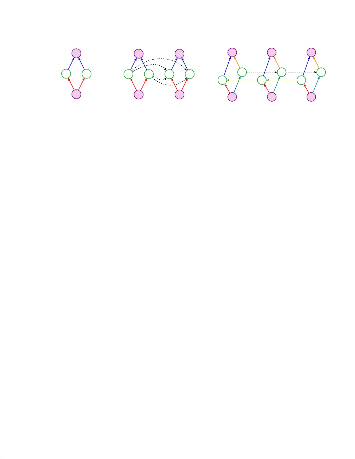
T raining Input-Output Recurren t Neural Net w orks through Sp ectral Metho ds Hanie Sedghi ∗ Anima Anandkumar † No v em b er 1, 2016 Abstract W e consider th e problem of training inp ut-output recurrent neural netw orks (RNN) for sequence labeling tasks. W e prop ose a no vel spectral approach for learning the netw ork parameters. It is based on decomposition of th e cross-momen t tensor betw een the output and a n on-linear transformatio n of the input, based on score functions. W e guara ntee consisten t learning with polyn omial sample and computational complexity un der transparen t conditions such as non-degeneracy of model parameters, p olynomial activ ations for the neurons, and a Marko vian evolution o f th e input sequence. W e also extend our results to Bidirectional RNN which uses b oth prev ious and future information to outp ut the label at each time p oin t, and is employ ed in man y NLP tasks such as POS tagging. Keyw ords: Recurrent ne ur al netw or ks, sequence labe ling , spectral metho ds , s c ore function. 1 In tro duction Learning with sequential data is widely encountered in domains such as na tural langua ge pro cessing, ge- nomics, speech recognition, video pro cessing, ﬁnancia l time series analysis, and so on. Recurrent neural net works (RNN) are a ﬂexible class of sequential mo dels whic h can memo rize past information, and se le c- tively pass it on acros s sequence steps o n m ultiple sca le s. How ever, training RNNs is challenging in practice, and backpropagation suﬀers from explo ding a nd v anishing gr adien ts as the length of the tra ining sequence grows. T o overcome this, either RNNs are trained o ver sho rt sequence s or incor por a te more complex archi- tectures s uc h as long s hort-term memories (LSTM). F or a detailed o verview of RNNs, see [20]. Figure 1 contrasts the RNN with a feedforward neural net work which has no memory . On the theoretica l front, understanding of RNNs is at best rudimentary . With the current tec hniques, it is not tractable to analyze the highly non-linea r state evolution in RNNs. Analysis of backpropagation is also intractable due to non-conv ex ity of the loss function, and in general, r eac hing the glo bal optim um is hard. Her e, w e take the ﬁr st steps tow ards addressing these challenging issue s . W e design nov el spectr a l metho ds fo r tra ining IO-RNN and B RNN mo dels. W e consider the class of input-output RNN or IO- RNN mo dels, where each input in the se quence x t has a n output lab el y t . These are useful for sequence lab eling tasks, which ha s many applica tions such as parts of sp eech (POS) tagging and named-entit y re cognition (NER) in NLP [21], motif ﬁnding in protein analysis [9], action reco gnition in videos [16], and so on. In addition, we a lso consider an extens io n of IO-RNN, viz., the bi-directional RNN or BRNN, ﬁr s t prop osed b y Sch uster and P aliwal [22]. This includes t wo classes of hidden neurons: the ﬁrst class r eceiv es recurrent co nnection from previous states, and the s econd class receives it from next steps. See Figure 1(c). BRNN is useful in NLP tas ks such a s POS ta gging, where both previous a nd next w ords in a sen tence have an eﬀect on lab eling the curr en t w ord. ∗ Allen institute F or Ar tiﬁcial In telligence. Email: han i es@al lenai.org † Unive r sit y of C al ifornia, Irvine. Em ail: a.anandkumar@uci.edu 1 Input Output Hidden Layer any t (a) NN Input Output Hidden Layer t = 2 t = 1 (b) IO-R NN Input Output Hidden Lay er x t x t − 1 x t +1 y t y t − 1 y t +1 z t − 1 (c) BRNN Figure 1: Graphical rep resen tation of a Neural Netw ork (NN) versus an Input -Output Recurren t Neu ral Net work (IO-RN N) and a Bidirectional R ecurren t Neu ral Netw ork (BRNN ) In this pap er, we dev elop novel sp ectral metho ds for training IO-RNN a nd BRNN mo de ls . Sp ectral metho ds have pr eviously b een emplo yed for unsuper vised lear ning of a ra ng e of laten t v aria ble mo dels such as hidden Markov models (HMM), topic mo dels, netw or k communit y mo dels, and so on [4]. The idea is to deco mpose moment matrices and tensors using computationa lly eﬃcie nt a lgorithms. The recovered comp onen ts of the tensor decompo sition y ield cons isten t estimates o f the model parameter s. Ho wev er, a direct application o f these techniques is ruled out due to non-linearity o f the activ atio ns in the RNN. Recently , Janzamin et a l. [15] derived a new fra mew ork for tra ining input-output mo dels in the sup ervised framework. It is bas e d on sp ectral decomp osition of moment tenso rs, obtained after certain non-linear trans - formations of the input. These no n- linear tra nsformations take the form of s c or e functions , whic h depend on generative mo dels of the input. This provides a new approach for transfer ring generative information, obtained through unsuper vised lea rning, into discriminative training on lab e le d samples. Based on the afore- men tioned appro ac h, Janzamin et al. [1 4] provided gua ranteed r isk b ounds for training t wo-lay er feedforward neural netw ork models w ith p olynomial sample a nd computational b ounds. The conditions for obtaining the r isk b ounds are mild: a s mall appr o ximatio n er ror for the targ et function under the given clas s of neural net works, a generative input mo del with a contin uous distr ibution, and general s igmoidal activ a tions at the neurons. W e pr opos e new spectral approaches for training IO-RNNs in b oth cla ssiﬁcation and r egression settings. The previous score function appro ac h for training feedfor w ar d net works (as describ ed ab ov e) do es not im- mediately extend, and there a re some non-trivial challenges: (i) Non-linear it y in a RNN is propa gated along m ultiple steps in the sequence, while in the tw o -lay er feedfor w ard netw o r k, non-linearity is applied only o nce to the input. It is not immediately clear on how to “ un tangle” a ll these non-linear ities and obtain g uaranteed estimates of the netw or k weight s. (ii) Learning bidirectional RNN s is even mor e challenging since recursive non-linearities are applied in both the directions, and (iii) Assumption of i.i.d. input a nd output training samples is no longer applicable, and analyzing concentration b ounds for samples genera ted from a RNN with non-linear state ev olution is challenging. W e addr ess a ll these c halle ng es concretely in this pap er. 1.1 Summary of Results Our main contributions are: (i) nov el approaches for training input-output RNN and bidirectional RNN mo dels using tenso r decompo sition metho ds, (ii) guar an teed recov er y of net work parameter s with po lynomial computational and sample complexity , and (iii) transpa ren t conditions for successful recovery based o n non- degeneracy of mo del parameters and b ounded ev olutio n of hidden states. Score function transformations: T raining input-output neural net works under arbitrary input is computationally hard. On the other hand, we show that training be c omes tractable thro ugh sp ectral metho ds when the input is gener ated fr om a proba bilistic mo del on a con tinuous state spa c e . This pap er can be considered as study of what it takes to uncov er the nonlinea r dynamics in the system. Since lea r ning 2 under arbitrar y input is extremely challenging, we seek to discover under what functions/infor mation of the input the problem b ecomes tr a ctable. Although this diﬀers from usual a pproach in training IO-RNNs, this is a promising ﬁrst s tep towards dem ystifying these widely-used models . W e show that with some knowledge of the input distribution, we can so lve the extremely hard pro ble m of training nonlinea r IO- RNNs. W e assume knowledge of scor e function forms, whic h corresp ond to nor malized deriv atives of the input probabilit y density function (p.d.f ). F or instance, if the input is standard Ga ussian, score functions are given b y the Hermite p olynomials. T he r e are man y unsup ervised appr o aches for estimating the scor e function eﬃciently , see App endix E.1. T o estima te the score function, one do es not need to estimate the density , and this distinction is especially crucia l for mo de ls wher e the normalizing constant or the p artition function is intractable to c ompute. Guarantees hav e b een derived for estimating s core functions of man y ﬂexible model classes suc h as inﬁnite dimensional exp onential families [26]. In addition, in many settings, we hav e con trol o ver designing the input distr ibution a nd our metho d is directly applicable. W e assume a Ma rk ovian mo del for the input sequence { x 1 , . . . , x n } on a con tinuous state space. F or a Marko via n mo del, the score function only dep ends o n the Markov kernel, a nd has a co mpact r e pr esen tatio n, as seen in Section 3.2. The metho d readily lea ds to higher order Marko v c hains. In the main pap er we discuss the ﬁr s t order Markov chain for notation simplicit y and dis c uss the extension in Appendix D.3. T ensor decomp osi tion: W e form cross-mo men ts betw een the output label a nd score functions of the input. F or a vector input, the ﬁrst order sc ore function is a v ecto r , second order is a matrix, and higher orders co rresp onds to tensors . Hence, the e mpir ical moments are tenso rs, and we p erform a CP tensor decomp osition to obtain the rank-1 comp onen ts. Eﬃcient algorithms for tenso r decompo s ition hav e been prop osed befor e , based on simple iterative up dates such as tensor p ow er method [4]. After so me simple manipulations on the components, we provide estimates of the netw or k par ameters of RNN mo dels. The ov erall algorithm in volv es simple linear a nd multilinear steps, is em barra ssingly par allel, and is practical to implemen t [29]. Reco very guaran tees: W e gua rant ee co nsisten t recov er y under (a low order ) p olynomial a nd co mputa- tional co mplex it y . W e consider the realizable s e tting when sa mples ar e gener ated by a IO-RNN or a BRNN under the following transpa ren t co nditio ns: (i) one hidden la yer of neurons with a polyno mia l activ a tion function, (ii) Ma rk ovian input sequence, (iii) full rank weigh t matr ices on input, hidden and output layers, and (iv) spectral norm bounds on the weight ma trices to ensure bounded state ev o lutio n. Currently , the q uestion of approximation bounds by a RNN with a ﬁxed num ber of neuro ns is not satisfactorily resolved [11] and it is v a lid to ﬁrst consider the realizea ble setting for this complex pr oblem. The p olynomial activ ations ar e a depa rture from the usual sigmoidal units, but they can also capture non- linear signal ev olution, and hav e been employ ed in diﬀeren t applications, e.g., [10], [30]. The Mar k ovian assumption on the input limits the extent of dep endence and allows us to derive concen tra tio n bounds for our e mpir ical moments. The full rank conditions on the weigh t matrices imply no n-degeneracy in the neura l representation: the weigh ts for any t wo neurons cannot linear ly combine to generate the weigh t of ano ther neuron. Suc h conditions hav e previously been der iv ed for sp ectral learning of HMMs and other laten t v a riable mo dels [4]. Moreover, it can b e easily relax ed b y cons idering higher or der momen t tens o rs, and is relev ant when we w a nt to have mor e neurons than the input dimension in our netw ork. The rank assumption on the o utput w eig h t ma tr ix implies a vector output of suﬃcien t dimensio ns, i.e., suﬃcient n umber of output classes. This can be relaxed to a scala r o utput, the details are given in Appendix E.2. The spectr al norm condition on the w eig ht matrices arises in the analys is o f c o ncen tra tio n b ounds for the empirical moments. Since w e as s ume p olynomial state evolution, it is important to ensure b ounded v alues of the hidden states, and this entails a b ound on the sp ectral norm of the w eig h t matr ic es. W e employ concentration bo unds for functions of Markovian input from [19, 18] and combine it with matrix Azuma’s inequa lit y [28] to o btain concentration of empiric al moment tensors. This implies lear ning RNNs with polynomia l sample complexity . Related w ork: The following works ar e dire ctly relev ant to this pape r . (a) Sp ectral approac hes for sequence learning: P r evious guara n teed appro ac hes for sequence learning mostly fo cus on the class of hidden Marko v mo dels (HMM). Anandkumar et al. [4] provide a tensor decomp osition metho d for learning the parameter s under non-deg eneracy co nditions, s imilar to ours. This framework is extended to more 3 general HMMs in [12]. While in a HMM, the rela tionship b etw een the hidden a nd observed v ariables can be mo deled as a linear one, in a RNN it is no n- linear. How e ver, in a IO-RNN, w e have both inputs and outputs, and that is helpful in handling the non-linear ities. (b) Input-output s equence mo de l s: A rich set of models based on RNNs ha ve b een employ ed in practice in a wide range of applications. Lipton et al. [20] provides a nice overview of these v ario us mo dels. Balduzzi a nd Ghifar i [8] recently apply physics based principles to design RNNs for sta bilizing gradients and getting b etter tra ining error. How ever, a rigorous analysis of these techniques is lacking. 2 Preliminaries Let [ n ] := { 1 , 2 , . . . , n } , and h u, v i denote the inner pro duct of v ector s u and v . F or sequence of n vectors z 1 , . . . , z n , we use the notation z [ n ] to denote the whole sequence. F or vector v , v ∗ m refers to element wise m th power of v . F or matrix C ∈ R d × k , the j -th co lumn is referred by C j or c j , j ∈ [ k ], the j th row is referred by C ( j ) or c ( j ) , j ∈ [ d ]. T hr oughout this paper, ∇ ( m ) x denotes the m th order deriv ative oper ator w.r.t. v ariable x . T ensor: A real m th or der tensor T ∈ N m R d is a member of the outer product of Euclidean spa ces R d . The diﬀeren t dimensions of the tensor are referred to as mo des . T ensor Reshaping: T 2 = Reshap e( T 1 , v 1 , . . . , v l ) means that T 2 is a tensor of order l that is made b y reshaping tensor T 1 such that the ﬁrst mode of T 2 includes modes of T 1 that are sho wn in v 1 , the second mo de of T 2 includes mo des of T 1 that ar e shown in v 2 and so o n. F or ex ample if T 1 is a tensor of order 5, T 2 = Reshape( T 1 , [1 2] , 3 , [4 5]) is a third order tensor, where its ﬁrst mo de is made b y c oncatenation of mo des 1 , 2 of T 1 and so on. T ensor rank: A 3rd order tenso r T ∈ R d × d × d is said to be rank-1 if it ca n b e written in the fo rm T = w · a ⊗ b ⊗ c ⇔ T ( i, j, l ) = w · a ( i ) · b ( j ) · c ( l ) , wher e ⊗ represents the outer pr o duct , and a, b, c ∈ R d are unit v ecto rs. A tensor T ∈ R d × d × d is s aid to hav e a CP (Candeco mp/ P ar afac) r ank k if it can b e (minimally) written as the sum of k rank-1 tensors T = P i ∈ [ k ] w i a i ⊗ b i ⊗ c i , w i ∈ R , a i , b i , c i ∈ R d . No te tha t v ⊗ p = v ⊗ v ⊗ v · · · ⊗ v , where v is rep eated p times . Deﬁnition 1 (Row-wise Krone ck er pro duct) F or matric es A, B ∈ R d × k , the Row-wise Kronecker pro d- uct ∈ R d × k 2 is deﬁne d as f ol lows. L et a ( i ) , b ( i ) b e r ows of A, B r esp e ctively. R ows of A ⊙ B ar e of t he form a ( i ) ⊗ b ( i ) . Note that our deﬁnition is diﬀer ent fr om usual deﬁnition of Kha tri-Rao pr o duct which is a c olumn-wise Kr one cker pr o duct . Deriv ativ e: F or function g ( x ) : R d → R with v ecto r input x ∈ R d , the m -th o rder der iv ative w.r.t. v ar iable x is denoted by ∇ ( m ) x g ( x ) ∈ N m R d (whic h is a m -th order tensor) suc h that h ∇ ( m ) x g ( x ) i i 1 ,...,i m := ∂ g ( x ) ∂ x i 1 ∂ x i 2 · · · ∂ x i m , i 1 , . . . , i m ∈ [ d ] . T ensor as m ulti linear fo rm: W e v iew a tenso r T ∈ R d × d × d as a m ultilinear form. Consider matrices M l ∈ R d × d l , l ∈ { 1 , 2 , 3 } . Then tensor T ( M 1 , M 2 , M 3 ) ∈ R d 1 ⊗ R d 2 ⊗ R d 3 is deﬁned as T ( M 1 , M 2 , M 3 ) i 1 ,i 2 ,i 3 := X j 1 ,j 2 ,j 3 ∈ [ d ] T j 1 ,j 2 ,j 3 · M 1 ( j 1 , i 1 ) · M 2 ( j 2 , i 2 ) · M 3 ( j 3 , i 3 ) . In particular, for vectors u, v , w ∈ R d , we ha ve 1 T ( I , v , w ) = X j,l ∈ [ d ] v j w l T (: , j, l ) ∈ R d , 1 Compare with the matri x case where for M ∈ R d × d , we hav e M ( I , u ) = M u := P j ∈ [ d ] u j M (: , j ) ∈ R d . 4 which is a multilinear combination of the tensor mo de-1 ﬁb ers. Similarly T ( u, v , w ) ∈ R is a m ultilinear combination of the tenso r entries, and T ( I , I , w ) ∈ R d × d is a linear combination of the tensor slices. 2.1 Problem F orm ulation W e consider a t wo-la yer input-output RNN, that includes b oth regres sion a nd cla ssiﬁcation settings : E [ y t | h t ] = A ⊤ 2 h t , h t = poly l ( A 1 x t + U h t − 1 ) , where p oly l ( · ) deno tes an element-wise polynomia l of order l , The input sequence x consists o f the vectors x t ∈ R d x .h t ∈ R d h , y t ∈ R d y and hence A 1 ∈ R d h × d x , U ∈ R d h × d h and A 2 ∈ R d h × d y . W e can learn the parameters of the mo del using our method. Our a lgorithm is called GLOREE (Gua rant eed Learning Of Recurrent nEura l nEtw o rks) and is sho wn in Algorithm 1. Throughout the pap e r, we ass ume that the p.d.f. o f the input sequence v anishes in the boundary (i.e., when a n y co ordinate of the input g o es to inﬁnity). This is also the assumption in [15]. W e consider the ca s e where input is a geometrically er godic Markov c hain. Then in order to hav e mixing and assure er go dic ity for the output, we need to impose additional constraints o n the mo del. 2.2 Review of Score functions As mentioned in the introductio n, our method builds on the metho d introduced by Janzamin et al. [1 5] called FEAST (F eature ExtrAction using Sco re function T ensors ). The go al of FEAST is to extrac t discriminative directions using the cross -momen t betw een the la bel and score function o f input. Sco re function is the normalized (higher order) deriv ative of p.d.f. of the input. Let p ( x ) denote the join t probability densit y function of ra ndom vector x ∈ R d . Janzamin et a l. [15] denote S m ( x ) as the m th order score function, given by S m ( x ) = ( − 1) m ∇ ( m ) x p ( x ) p ( x ) , (1) where ∇ ( m ) x denotes the m th order der iv ative op erator w.r.t. v ar iable x . It can also b e der iv ed using the recursive form S 1 ( x ) = −∇ x log p ( x ) , (2) S m ( x ) = −S m − 1 ( x ) ⊗ ∇ x log p ( x ) − ∇ x S m − 1 ( x ) . The impo rtance of scor e function is that it provides a der iv ative o pera tor. J anzamin et al. [1 5] prov ed that the cross-mo men t b etw e en the la bel and the sco re function of the input yields the infor mation reg arding deriv a tiv e of the lab el w.r.t. the input. Theorem 1 (Yie l ding di ﬀ eren tial op erators [15]) L et x ∈ R d x b e a r andom ve ctor with joint density function p ( x ) . Supp ose the m th or der sc or e function S m ( x ) deﬁne d in (1 ) ex ist s. Consider any or der m c on- tinuously diﬀer ent iable tensor fun ction G ( x ) : R d x → N r R d y . Then, un der some m ild re gularity c onditions 2 , we have E [ G ( x ) ⊗ S m ( x )] = E h ∇ ( m ) x G ( x ) i . 2 Consider an y contin uously diﬀeren tiable tensor function G ( x ) : R d x → N r R d y satisfying the regularity condition such that all the entries of ∇ ( i ) x G ( x ) ⊗ S m − i − 1 ( x ) ⊗ p ( x ), i ∈ { 0 , 1 , . . . , m − 1 } , go to zero on the b oundaries of support of p ( x ). 5 3 Extension of score function to inp ut s equences 3.1 Score function form for RNN W e now extend the notion of sco r e function to handle sequence data with non i.i.d. samples. W e denote the score function at eac h time step t in the sequence as S m ( z [ n ] , t ), where z [ n ] := z 1 , z 2 , . . . , z n , and it is deﬁned below. Theorem 1 can b e readily mo diﬁed to Lemma 2 (Score function form for input sequence) F or ve ctor se quenc e z [ n ] = { z 1 , z 2 , . . . , z n } , let p ( z 1 , z 2 , · · · , z n ) and S m ( z [ n ] , [ n ]) re sp e ctively denote the joint density fun ct ion and the c orr esp onding m th or- der sc or e function. Then, under some mild r e gularity c onditions, for al l c ontinuou s ly diﬀe r ent iable functions G ( z 1 , z 2 , . . . , z n ) , we ha ve E [ G ( z 1 , z 2 , . . . , z n ) ⊗ S m ( z [ n ] , t )] = E h ∇ ( m ) z t G ( z 1 , z 2 , . . . , z n ) i , wher e ∇ ( m ) z t denotes the m th or der d erivative op er ator w.r.t. z t , S m ( z [ n ] , t ) = ( − 1) m ∇ ( m ) z t p ( z 1 , z 2 , . . . , z n ) p ( z 1 , z 2 , . . . , z n ) . (3) 3.2 Score function form for Mark ov c hains W e ass ume a Marko vian mo del for the input seq ue nc e , and deriv e compact score function for ms for (3). Note that this form can be readily expanded to higher-or der Ma rko v chains. Lemma 3 (Score funct i on for ﬁrst-order Mark o v Chains) L et the input s e quen c e { x i } i ∈ [ n ] b e a ﬁrst- or der Marko v chain. The sc or e function in (3) simpli ﬁes as S m ( x [ n ] , i ) = ( − 1) m ∇ ( m ) x i [ p ( x i +1 | x i ) p ( x i | x i − 1 )] p ( x i +1 | x i ) p ( x i | x i − 1 ) . (4) The pro of follows the deﬁnition of ﬁr st-order Mar kov chain and Equatio n (3). 4 Algorithm and G uaran tees In this pap er, we hav e functions which map input sequence x 1 , . . . x n to an output sequence y 1 , . . . , y n . By assuming a structure d fo rm of function mapping in ter ms of IO-RNN, we can hop e to recov er the function parameters eﬃciently . W e exploit the score function forms de r iv ed a bov e to compute partial deriv atives of the output seq uence.W e ﬁrst start with some simple intuitions. 4.1 Preliminary insigh ts Generalized linear mo del : Before considering the RNN, co nsider a simple gene r alized linear mo del with i.i.d. samples: E [ y | x ] = A ⊤ 2 σ ( A 1 x ), where A 1 is the weight matrix and σ ( · ) is element -wis e activ ation. Here, the partial der iv ative of E [ y | x ] w.r .t. x has a linear relatio nship with the w eight matrices A 1 and A 2 , i.e., E [ ∇ x E [ y | x ]] = E [ A ⊤ 2 ∇ x σ ( A 1 x )] = A ⊤ 2 E [ σ ′ ( A 1 x )] A 1 . (5a) E [ y ⊗ S 2 ( x )] = E [ ∇ 2 x E [ y | x ]] = X i ∈ d h µ i A ( i ) 2 ⊗ A ( i ) 1 ⊗ A ( i ) 1 . (5b) The ﬁrst partial deriv ative is obtained by forming the cross moment E [ y ⊗ S 1 ( x )], as given by Theor em 1. The form in (5a) yields A 1 and A 2 up to a linea r transformation. But, by computing seco nd o rder deriv atives, we 6 can recover A 1 and A 2 , up to sca ling of their rows. The second order der iv ative ha s the form in (5b). The tensor decomp osition in [4 ] uniq ue ly recov ers A 1 , A 2 up to sc a ling o f r o ws, under full ro w ra nk as s umptions. Reco vering input-output w ei g h t matrices in IO-RNN: The ab ov e in tuition for GL M r eadily carr ies ov er to IO-RNN. Recall that the IO-RNN has the form E [ y t | h t ] = A ⊤ 2 h t , h t = poly l ( A 1 x t + U h t − 1 ) , where poly l denotes an y poly no mial function of degree a t mo s t l . Suppo se we hav e access to partia l deriv atives E [ ∇ x t E [ y t | h t ]] a nd E [ ∇ 2 x t E [ y t | h t ]], then they have the same forms as (5a) and (5b). 3 This is because h t do es not dep end on x t − 1 given x t , h t − 1 . Th us, the weight matrices A 1 and A 2 can be eas ily recovered b y forming E [ y t ⊗ S 2 ( x [ n ] , t )], a s g iv en b y (3), and it has a compact form for Mar k ovian input in (4). Note that this intuition holds for any non-linear elemen t-wise activ atio n function, and w e do no t requir e it to be a p olynomia l at this s tage. Reco vering hi d de n state transition matrix in IO-RNN: Recov ering the transitio n matrix U is m uch more challenging as we do not ha ve access to hidden state sequence h [ n ]. Thus, we cannot readily form partial deriv atives of the form ∇ m h t − 1 E [ y t | h t ]. Also, the no n- linearities ge t r e cursively pro pagated along the chain. Here, we provide an algor ithm that works for any p olynomial activ atio n function o f ﬁxed degr e e l . The main idea is that we attempt to recov er U b y considering pa rtial der iv atives ∇ m x t − 1 E [ y t | h t ], i.e., ho w the previous input x t − 1 aﬀects current output y t . At ﬁrst g lance, this a ppears complicated and indeed, the v ar ious ter ms are hig hly coupled and w e do not ha ve a nice CP tensor deco mpositio n form. How ever, w e can prov e that when the deriv ative order m is suﬃciently large, a nice CP tensor fo rm emer g es out, and this m depends on the deg ree l of the poly nomial ac tiv ation. F or simplicit y , w e provide in tuitions for the quadratic activ ation function ( l = 2). Now, y t is a degree- 4 po lynomial function of x t − 1 , since the activ ation function is applied twice. By consider ing four th order deriv a tiv e ∇ 4 x t − 1 E [ y t | h t ], many coupled ter ms v anish sinc e they corres pond to po lynomial functions of degree less than 4. The surviving ter m has a nice CP tensor form, a nd we can recov er U eﬃcien tly fro m it. Note that this fourth order pa rtial deriv ative ca n b e computed eﬃciently using fourth order score function and forming the cr oss-moment E [ y t ⊗ S 4 ( x [ n ] , t − 1)]. The precise alg orithm is given in Algorithm 1. 4.2 T raining IO-RNNs W e now provide our a lgorithm for training IO-RNNs. In this pap er we consider v ector output a nd po lynomial activ atio n fun ctio ns of an y or der l ≥ 2. F o r s implicity of notation, we ﬁrst discuss the case for quadra tic activ atio n function. O ur algorithm is ca lled GLOREE (Guaranteed Learning Of Recur ren t nEura l nEt works) and is shown in Alg orithm 1 for quadratic activ ation function. The gener al a lgorithm and analy s is for l ≥ 2 is s ho wn in App endix C.1. F o r completeness, w e handle the linear case in Appendix E .3. W e also cover the case where o utput y is a scalar (e.g. a binary label) in App endix E.2. Now, we consider an RNN with quadratic activ ation function a nd vector o utput. Let E [ y t | h t ] = A ⊤ 2 h t , h t = poly 2 ( A 1 x t + U h t − 1 ) , (6) where x t ∈ R d x , h t ∈ R d h , y t ∈ R d y and A 1 ∈ R d h × d x , U ∈ R d h × d h , A 2 ∈ R d h × d y . W e ca n lea rn the parameters of the mo del using GLOREE . Let n be the windo w size for RNN. Theorem 4 (Learning parameters of RNN for quadratic ac tiv ation function) L et R b e the mo del describing the IO-RN N as in (6) . Assuming t hat A 1 , A 2 , U ar e ful l c olumn r ank, we c an r e c over t he p ar am- eters of R using Algo rithm 1 (GLOREE). 3 Note that h t is a (pol ynomial ) function of x t so E [ y t | h t ] = pol y ( x t , h t − 1 ). A lso the expectation is w.r.t. all v ariables x 1 , . . . , x t , and thus, the dependence to h t − 1 is also av eraged out since it is a function of x 1 , . . . , x t − 1 . 7 Algorithm 1 GLOREE (Guara n teed Learning Of Recurrent nEura l nEtw orks) for v ector input and quadratic function (General cas e shown in Algorithm 3 in Appendix C.1 ). input L a beled samples { ( x i , y i ) : i ∈ [ n ] } from IO-RNN mo del in Figur e 1. 1: Co mpute 2nd- o rder sco re function S 2 ( x [ n ] , i ) of the input sequence a s in Equation (4). 2: Co mpute b T := b E [ y i ⊗ S 2 ( x [ n ] , i )]. The empirical a verage is ov er a single sequence. 3: { ˆ w, ˆ R 1 , ˆ R 2 , ˆ R 3 } = tensor decompo sition( b T ); see Appendix F. 4: ˆ A 2 = ˆ R 1 , ˆ A 1 =  ˆ R 2 + ˆ R 3  / 2. 5: Co mpute 4th-o rder sco re function S 4 ( x [ n ] , i ) of the input sequence a s in Equation (4). 6: Co mpute b T 2 := ˆ E [ y t ⊗ Reshap e (( S 4 ( x [ n ] , t − 1) , [1 2] , [3 4])]. 7: { ˆ w, ˆ R 1 , ˆ R 2 , ˆ R 3 } = tensor decompo sition( b T 2 ); see App endix F. 8: ˆ U = ˜ R h ˆ A 1 ⊙ ˆ A 1 i † , ˜ R =  ˆ R 2 + ˆ R 3  / 2. ⊙ is row-wise Kroneck er pro duct as in Deﬁnition 1. 9: return ˆ A 1 , ˆ A 2 , ˆ U . Pro of Sketc h: W e hav e the following prop erties for an IO-RNN: E [ y t ⊗ S 2 ( x [ n ] , t )] = 2 X i ∈ d h A ( i ) 2 ⊗ A ( i ) 1 ⊗ A ( i ) 1 . (7) Hence, w e can r eco ver A 1 , A 2 via tensor deco mpositio n, assuming that they ar e full row ra nk. In o rder to learn U w e form the tensor E [ y t ⊗ S 4 ( x t − 1 )], and under quadra tic a ctiv ations, w e hav e E [ y t ⊗ Reshap e( S 4 ( x [ n ] , t − 1) , [1 2] , [3 4])] = X i ∈ d h A ( i ) 2 ⊗ [ U ( A 1 ⊙ A 1 )] ( i ) ⊗ [ U ( A 1 ⊙ A 1 )] ( i ) . Hence, w e ca n recov er U ( A 1 ⊙ A 1 ) via tensor decomp osition. Since A 1 is previously r ecov ered using (7), and ( A 1 ⊙ A 1 ) † exists due to full rank a ssumption, we ca n r ecov er U . Th us, Algorithm 1 (GLORE E) consistently recov ers the para meters of IO-RNN under quadra tic activ ations. F or pro o f, see Appendix B.1. 4.3 T raining Bidirectional RN Ns Bidirectional Recurr en t Neur al netw ork was ﬁr st prop osed by Sch uster a nd Paliwal [22]. Here there are t wo groups of hidden neurons.The ﬁrst group receives recurrent connections from previo us time steps while the other from the next time steps. The follo wing equations describe a B RNN E [ y t | h t , z t ] = A ⊤ 2  h t z t  , h t = f ( A 1 x t + U h t − 1 ) , z t = g ( B 1 x t + V z t +1 ) , (8) where h t and z t denote the neurons that rece ive forward and ba c kward connections, resp ectively . Note that BRNNs canno t b e used in online settings as they require knowledge of the future steps. How ever, in v ar ious na tural language pro cessing applications suc h as part o f s peech BRNNs are eﬀectiv e mo dels since they consider b oth past and future words in a s en tence. W e can learn the parameters of bidir ectional RNN by mo difying our earlier algor ithm. F or no ta tion sim- plicit y , Algorithm 2 sho ws the case for quadra tic activ ation functions f ( · ) and g ( · ). The general p olynomial function is c onsidered in Algorithm 4 in App e ndix C.2. Let us provide s ome in tuitions. If we only had forward or backw ar d connections , we would directly apply our previo us metho d in GLOREE . F or backw ar d connections , the only diﬀerence would be to use der iv atives of E [ y t | h t , z t ] w.r .t. x t +1 to learn the tr a nsition ma tr ix V . Now tha t we have b oth hidden neurons mixing to yield the output vector y t , the cross- momen t tensor T = E [ y i ⊗ S 2 ( x [ n ] , i )] has a CP dec ompositio n where the factor matrix for the ﬁr st mode is A 2 , i.e., the tensor has a sp eciﬁc form: T = A ⊤ 2  T h T z  , where T h 8 Algorithm 2 GLOREE-B (Guaranteed Lea rning Of Recurrent nEural nE t works-Bidirection case) for quadratic activ ation function (general cas e is shown in Algorithm 4 ). input L a beled samples { ( x i , y i ) : i ∈ [ n ] } from (8). input 2 nd-order s core function S 2 ( x [ n ] , [ n ]) o f the input x ; see E q uation (1) for the deﬁnition. 1: Co mpute b T := ˆ E [ y i ⊗ S 2 ( x [ n ] , i )]. The empirical av erage is ov er a single sequence. 2: { ( ˆ w , ˆ R 1 , ˆ R 2 , ˆ R 3 } = tensor decompo sition( b T ); see Appendix F. 3: ˆ A 2 = ˆ R 1 . 4: Co mpute ˜ T = b T ((( ˆ A 2 ) ⊤ ) − 1 , I , I ). F or deﬁnition of multilinear form see Section 2. 5: { ( ˆ w , ˆ R 1 , ˆ R 2 , ˆ R 3 } = tensor decompo sition( ˜ T ); 6: ˆ C = ( ˆ R 2 + ˆ R 3 ) / 2. 7: ˆ C =  ˆ A 1 ˆ B 1  . 8: Co mpute 4th-o rder sco re function S 4 ( x [ n ] , t − 1) of the input s equence as in Equation (4). 9: Co mpute b T = ˆ E [ y t ⊗ Reshap e (( S 4 ( x [ n ] , t − 1) , [1 2] , [3 4])]. 10: { ˆ w, ˆ R 1 , ˆ R 2 , ˆ R 3 } = tensor decompo sition( b T ); see Appendix F. 11: ˆ U = ˜ R h ˆ A 1 ⊙ ˆ A 1 i † , ˜ R =  ˆ R 2 + ˆ R 3  / 2. ⊙ is row-wise Kroneck er pro duct as in Deﬁnition 1. 12: Repea t lines (8)-(1 1) with S 4 ( x [ n ] , t + 1) instead of S 4 ( x [ n ] , t − 1) to recover ˆ V . 13: return ˆ A 1 , ˆ A 2 , ˆ B 1 , ˆ U , ˆ V . corres p onds to the tenso r incorp orating columns of A 1 and T z incorp orates columns of B 1 . Hence, under full rank ass umption, as b efore, we can recov er A 2 . Next, we can inv ert A 2 to rec over T h and T z . W e decomp ose them to r ecov e r A 1 and B 1 . The s teps for recovering U a nd V remains the same a s b efore in GLOREE . The only diﬀerence is to use deriv atives of E [ y t | h t , z t ] w.r.t. x t +1 to learn V . Theorem 5 (T raining BRN N) L et B b e the BRNN mo del in (8) . A ssuming that A 1 , A 2 , B 1 , U, V ar e ful l c olumn r ank, we c an r e c over the p ar ameters of B using Algo rithm 2. F o r pro of, see Appendix B.2. 4.4 Analysis of GLOREE Sample Complexit y: In order to ana ly ze the sample complexit y , we ﬁrst need to pr ove concentration b ound for the cr oss-moment tensor, then we use analysis of the tensor decompositio n to show the that sample complexit y is a low o r der po lynomial o f co rresp onding parameters . Assumptions : 1. Bounded hidde n v ariables : since w e assume a polynomia l activ ation function, the hidden state h t can grow in an un b ounded manner. T o av oid this we need the follo wing: (a) Without los s of gene r alit y , w e assume that the input seq uence is b ounded by 1 with high proba - bilit y , k x i k < 1 ∀ i ∈ [ n ] (b) Ass ume tha t k A 1 k + k U k ≤ 1. (c) k A 2 k is b ounded. 2. Concen tration of mom en t tensor: Deriving concen tra tion b ound for the cross-moment tensor is a bit more inv olved since w e ha ve a non-i.i.d. sequence. (a) The input sequence is a geometrica lly ergo dic Mar k ov chain. (b) If the activ atio n function is a p olynomial of order l , w e need k U k ≤ 1 /l . (c) kS 2 ( x [ n ] , t ) k is a b ounded v alue. 9 (d) T he input sequence is a ﬁrst order Marko v chain. (e) k∇ x i S 2 ( x [ n ] , t ) k , i ∈ { t − 1 , t, t + 1 } is bounded by some v alue γ . 4 3. Uniqueness in tensor decomp osition: (a) weight ma trices A 1 , U, A 2 are full co lumn rank, i.e., neurons are not redundant. Let G b e the geometric ergo dicit y and θ is the co ncen tratio n co eﬃcient of the input Mark ov c hain (see Appendix D for deﬁnition). W e hav e that: Theorem 6 (Sampl e Compl exit y for GLOREE) Assu me the c onditions ab ove ar e met. Supp ose the sample c omplexity n is ˜ O ( d x , d y , d h , G, ǫ − 2 , 1 1 − θ , σ − 1 min ( A 1 ) , σ − 1 min ( A 2 ) , σ − 1 min ( U )) , then for e ach wei ght matrix c olumn A ( i ) 1 , U ( i ) , A ( i ) 2 , i ∈ [ d h ] , we have that k b A ( i ) 1 − A ( i ) 1 k ≤ ǫ, i ∈ [ d h ] , k b U ( i ) − U ( i ) k ≤ ǫ, i ∈ [ d h ] , k b A ( i ) 2 − A ( i ) 2 k ≤ ǫ, i ∈ [ d h ] . Pro of Sketc h: The pro of has t wo main parts. First, we need to prove a concentration bound for the moment tensor. Second, w e can readily use the analys is of tensor deco mpositio n from earlier w o r ks such a s [4, 14] to compute the sample co mplexit y for this moment tenso r. Since the ﬁrs t part is the co n tribution of this paper , here w e focus on that. In order to pr o ve the concen tra tion b ound for the momen t tensor, note that our input sequence x [ n ] is a geometrically ergo dic Markov chain. W e can think of the empirical moment ˆ E [ y t ⊗ S m ( x [ n ] , t )] a s functions ov er the s amples x [ n ] of the Ma rk ov chain. Note that this ass umes h [ n ] and y [ n ] as deterministic functions of x [ n ], and our analysis c a n b e extended when there is a dditional randomnes s. Ko ntorovic h and W eiss [18] provide the result fo r scalar functions and this is an extensio n of that result to matr ix-v alued functions. W e use Assumptions 1(a)-(c) to ensure a bounded hidden v ariable. Next, b y leveraging Assumptions 2(a)-2(e) we prov e that the cross-mo men t tenso r satisﬁes Lipsc hitz prop ert y , which pa ves the w ay for proving the concentration b ound. F o r details, see Appendix D. Computational Complexity : The co mputational complexit y of o ur method is related to the complexity of the tensor deco mposition metho ds. See [4, 14] for a detailed discussio n. It is po pular to p erform the tensor decompo sition in a sto c hastic manner by splitting the data into mini-batches and reducing computational complexity . Sta r ting with the ﬁrst mini-batc h, we p erform a small n umber of tensor p ow er iterations, and then use the result as initialization for the next mini-batch, and so on. W e assume that score function is given to us in an eﬃcient form. Note that if we can write the cross -momen t tensor in terms of summation o f r ank-1 components, we do not need to for m the whole tensor explicitly . As an example, if input follows Gaussian distribution, the score function has a simple p olynomial form, and the computational complexity of tensor decompo sition is O ( nd h d x R ), wher e n is the n umber of samples a nd R is the n umber of initializations for the tensor decomp osition. Similar argument follows when the input is mixture of Gauss ian distributions. 4 W e need mil der assumptions than 2(d)-2(e). F or details see App endix D.3. 10 5 Conclusion This w ork is a ﬁrst step tow ards answ ering c halleng ing questions in sequenc e mo deling. W e prop ose the ﬁrst metho d that can recover para meters of IO-RNN as w ell as BRNN with guarantees. Many of the assumptions can b e rela xed, e.g., here we assumed IO - RNNs with alig ned inputs and o utputs. W e can r elax this assumption to obtain more general RNNs. This pap er o pens up a new hor izon for future research, such as extending this framework to HMMs and general settings and analysis under non-sta tionary inputsW e ha ve assumed the realiza ble setting where samples are g enerated from a RNN. The question of approximation b o unds b y a RNN with a ﬁxed num b er of neurons is an in teresting problem. Ac knowled gmen t The authors thank Ma jid Janza min for discussions on s a mple complexity and constructive comments on the draft. W e thank Ashish Sabha rw a l for editorial comments o n the dr aft. This work w a s done during the time H. Sedghi w as a visiting researcher a t Universit y of California, Irvine and w as s upported b y NSF Car eer aw ard F G158 90. A. Anandkumar is suppor ted in part b y Microso ft F aculty F ellowship, NSF Career a ward CCF-1254 106, ONR aw ard N00014- 14-1-06 65, AR O YIP aw a r d W911NF-13 -1-0084 , and AF O SR YIP aw ar d F A95 50-15-1 -0221. References [1] Guilla ume Alain and Y oshua Bengio. What regularized auto-e nc o ders learn from the data generating distribution. arXiv pr eprint arXiv :1211.424 6 , 20 12. [2] A. Anandk uma r, R. Ge, D. Hsu, S. M. K ak ade, and M. T elg a rsky . T ensor decomp ositions for learning latent v ar ia ble mo dels. J. of Mach ine L e arning Rese ar ch , 15:277 3–2832 , 2 014. [3] Anima Anandkumar, Yi-k ai Liu, Daniel J Hsu, Dean P F oster, a nd Sham M Kak a de. A sp ectral algorithm for laten t dirichlet allo cation. In A dvanc es in Neur al Information Pr o c essing Systems , pa ges 917–9 25, 20 12. [4] Anima Anandkumar, Rong Ge, Daniel Hsu, Sham M. Ka k ade, and Matus T elgar sky . T ens or decom- po sitions for learning la tent v aria ble mo dels. Journal of Machine L e arning R ese ar ch , 15:277 3 –2832, 2014. [5] Anima Anandkumar , Rong Ge, and Ma jid Janzamin. Sample Complexity Analys is for Learning Over- complete Latent V aria ble Mo dels thro ugh T ensor Metho ds. arXiv pr eprint arXiv: 1408.0553 , Aug. 2014. [6] Anima Anandkumar, Ro ng Ge, and Ma jid J anzamin. Guara n teed No n-Orthogonal T ensor Deco mposi- tion v ia Alternating Rank- 1 Upda tes. arXiv pr eprint a rXiv:1402.518 0 , F eb. 2014. [7] K am yar Azizzadenesheli, Alessa ndro Lazar ic, and Anima Anandkumar . Reinforc emen t learning o f po mdp’s us ing sp ectral methods. arXiv pr eprint arXiv:16 02.07764 , 2016. [8] David Balduzzi and Muhammad Ghifari. Strongly-typed recurr en t neural net works. arXiv pr eprint arXiv:160 2.02218 , 2016. [9] Asa Ben-Hur and Douglas Brutlag. Sequence motifs: highly predictive featur e s of pro tein function. In F e ature Ext r action , pages 6 25–645. Springer , 200 6. [10] D. Chen and C. Manning. A fast and accura te dep endency parser using neura l netw or ks. In EMNLP , pages 740–750, 201 4 . 11 [11] Barbar a Hammer. On the approximation c a pabilit y of recurrent neura l net works. Neu r o c omput ing , 3 1 (1):107–1 23, 20 00. [12] Qingqing Huang, Rong Ge, Sham Kak ade, a nd Mun ther Dahleh. Minimal r ealization problem for hidden marko v models. In Communic ation, Contr ol, and Comp u t ing (A l lerton), 2014 52nd Annual Al lerton Confer enc e on , pages 4–11 . IE EE, 2014. [13] Aap o Hyv¨ arinen. Estimation of no n- normalized statistical mode ls by score matc hing. In Journal of Machine L e arning R ese ar ch , pages 6 95–709 , 2005. [14] M. Janzamin, H. Sedghi, and A. Anandkumar. Beating the Perils of Non-Conv ex ity: Guar an teed T ra ining of Neural Net works using T enso r Metho ds. Pr eprint availa ble on arXiv:1506. 08473 , June 2015. [15] Ma jid Janzamin, Hanie Sedghi, and Anima Anandkumar. Score F unctio n F eatures for Discriminative Learning: Matrix and T ensor F rameworks. arXiv pr eprint arXiv: 1412.2863 , Dec. 201 4. [16] Andrej K arpathy , George T o derici, Sanketh Shetty , Thoma s Leung, Rahul Sukthank a r, and Li F ei- F ei. La rge-scale video c lassiﬁcation with conv olutiona l neural netw orks . In Pr o c e e dings of the IEEE c onfer enc e on Comp u t er Vision and Pattern R e c o gnition , pages 17 25–1732 , 2014. [17] George Konidaris and Finale Doshi-V elez. Hidden parameter markov decision pro cesses: An emerging paradigm for mo deling families of r elated tasks. In 2014 AA AI F al l Symp osium Series , 2014 . [18] Aryeh K on tor ovich and Roi W eiss. Unifor m c herno ﬀ and dvoretzky-kiefer -w olfowitz-type inequalities for marko v chains and related process es. Journal of Applie d Pr ob ability , 51(4):11 00–1113 , 2 014. [19] Leonid Aryeh Ko n torovich, Kavita Ramana n, et al. Concentration inequalities for dep endent random v ar iables via the martingale metho d. The Annals of Pr ob ability , 36(6):21 26–215 8, 2008. [20] Zachary C Lipton, John Ber k owitz, and Charles Elk an. A c r itical review of r e c urrent neural netw or ks for sequence lea rning. arXiv pr eprint arXiv: 1506.0001 9 , 2015. [21] C. Manning and H. Sch¨ utze. F oundations of statistic al natur al language pr o c essing , v olume 9 99. MIT Press, 1999. [22] Mike Sch uster a nd Kuldip K Paliwal. Bidirec tio nal recurr en t neur al netw or ks. Signa l Pr o c essing, IEEE T ra nsactions on , 45 (11):2673– 2681, 1997. [23] Hanie Sedghi and Anima Anandkumar. P rov a ble metho ds for training neural netw orks with sparse connectivity . NIPS workshop on De ep L e arning and R epr esentation L e arning , Dec. 2014. [24] L. Song, A. Anandkumar, B. Dai, and B. Xie. Nonpar ametric es timation of m ulti-view latent v ariable mo dels. arXiv pr eprint arXiv:1311.3 287 , Nov. 201 3 . [25] D. Spielman, H. W a ng , and J. W r igh t. Exact recovery of spar sely-used dictionaries. In Confer enc e on L e arning Th e ory , 201 2 . [26] Bharath Srip erum budur, K enji F ukumizu, Rev ant Kumar, Arthur Gretton, and Aap o Hyv¨ arinen. Den- sity estimation in inﬁnite dimensional exp onential families. arXiv p r eprint arXiv: 1312.3516 , 2 0 13. [27] Kevin Swersky , David Buchm a n, Nando D F reitas, Benjamin M Marlin, et a l. On auto enco ders and score matching for energ y base d mo dels. In Pr o c e e dings of the 28th International Confer enc e on Machine L e arning (ICM L-11) , pag es 1201 –1208, 2011 . [28] J. T r opp. User-frie ndly ta il b ounds for sums of random ma trices. F oundations of Computational Math- ematics , 12(4):389–4 3 4, 201 2. 12 [29] Yining W a ng, Hsiao-Y u T ung, Alexander Smola, a nd Anima Anandkumar. F as t a nd guaranteed tensor decomp osition v ia sketchin g . In Pr o c. of NIPS , 2015. [30] Qizhe Xie, Kai Sun, Su Zh u, Lu Chen, and Kai Y u. Recurre nt p olynomial net work for dialo gue state tracking with misma tched semantic pars e r s. In 16th A nn ual Me eting of the Sp e cial Inter est Gr oup on Disc ourse and Dialo gue , page 295, 20 15. A Notation F or completeness, all the notation required in the pap er and Appendices are g athered he r e as well. Let [ n ] := { 1 , 2 , . . . , n } , a nd k u k denote the ℓ 2 or Euclidean norm of vector u , a nd h u, v i denote the inner pro duct of v ectors u and v . F or sequence of n vectors z 1 , . . . , z n , w e use the notation z [ n ] to denote the whole sequence. F o r v ector v , v ∗ m refers to element wise m th power of v . F or matrix C ∈ R d × k , the j -th column is referred by C j or c j , j ∈ [ k ], the j th row is referr ed b y C ( j ) or c ( j ) , j ∈ [ d ] and k C k deno tes the sp ectral norm of matrix C . Throughout this pap er, ∇ ( m ) x denotes the m th order der iv ative op erator w.r.t. v ar iable x . T ensor: A real m th or der tensor T ∈ N m R d is a mem b er of the outer product of Euclidean spaces R d . The diﬀeren t dimensions of the tensor are referr ed to a s mo des . F o r instance, for a matrix, the ﬁr s t mo de refers to co lumns and the second mo de refers to rows. T ensor matricization: F or a third order tensor T ∈ R d × d × d , the matricized v ersio n alo ng ﬁrst mo de denoted b y M ∈ R d × d 2 is deﬁned suc h that T ( i, j, l ) = M ( i, l + ( j − 1) d ) , i, j, l ∈ [ d ] , (9) and w e use Ma t to show matricizatio n, i.e., M = ( M at )( T ) T ensor Reshaping: T 2 = Reshap e( T 1 , v 1 , . . . , v l ) means tha t T 2 is a tensor of order l that is made b y reshaping tensor T 1 such that the ﬁrst mode of T 2 includes modes of T 1 that are sho wn in v 1 , the second mo de of T 2 includes mo des of T 1 that ar e shown in v 2 and so o n. F or ex ample if T 1 is a tensor of order 5, T 2 = Reshape( T 1 , [1 2] , 3 , [4 5]) is a third order tensor, where its ﬁrst mo de is made b y c oncatenation of mo des 1 , 2 of T 1 and so on. T ensor rank: A 3rd or der tenso r T ∈ R d × d × d is said to b e r ank-1 if it can b e written in the form T = w · a ⊗ b ⊗ c ⇔ T ( i , j, l ) = w · a ( i ) · b ( j ) · c ( l ) , (10) where ⊗ r epresents the outer pr o duct , and a, b, c ∈ R d are unit v ectors . A tenso r T ∈ R d × d × d is said to ha ve a CP (Candecomp/ P ar afac) ra nk k if it can be (minimally) written as the sum of k rank-1 tensor s T = X i ∈ [ k ] w i a i ⊗ b i ⊗ c i , w i ∈ R , a i , b i , c i ∈ R d . (11) Note that v ⊗ p = v ⊗ v ⊗ v · · · ⊗ v , where v is repea ted p times. Deﬁnition 2 (Row-wise Krone ck er pro duct) F or matric es A, B ∈ R d × k , the Row-wise Kronecker pro d- uct ∈ R d × k 2 is deﬁne d b elow      a (1) a (2) . . . a ( k )      ⊙      b (1) b (2) . . . b ( k )      =      a (1) ⊗ b (1) a (2) ⊗ b (2) . . . a ( k ) ⊗ b ( k )      , 13 wher e a ( i ) , b ( i ) ar e r ows of A, B r esp e ctively. N ote that our deﬁnition is diﬀer ent fr om usual deﬁnition of Khatri-R ao pr o duct whic h is a c olumn - wise Kr one cker p r o duct (is p erforme d on c olumns of matric es). T ensor as m ulti linear form: W e view a tenso r T ∈ R d × d × d as a m ultilinear for m. Consider matrices M l ∈ R d × d l , l ∈ { 1 , 2 , 3 } . Then tensor T ( M 1 , M 2 , M 3 ) ∈ R d 1 ⊗ R d 2 ⊗ R d 3 is deﬁned as T ( M 1 , M 2 , M 3 ) i 1 ,i 2 ,i 3 := X j 1 ,j 2 ,j 3 ∈ [ d ] T j 1 ,j 2 ,j 3 · M 1 ( j 1 , i 1 ) · M 2 ( j 2 , i 2 ) · M 3 ( j 3 , i 3 ) . (12) In particular, for vectors u, v , w ∈ R d , we ha ve 5 T ( I , v , w ) = X j,l ∈ [ d ] v j w l T (: , j, l ) ∈ R d , (13) which is a multilinear combination of the tensor mo de-1 ﬁb ers. Similarly T ( u, v , w ) ∈ R is a multilinear combination of the tenso r entries, and T ( I , I , w ) ∈ R d × d is a linear combination of the tensor slices. Deriv ativ e: F or function g ( x ) : R d → R with vector input x ∈ R d , the m -th order deriv ative w.r.t. v ar iable x is deno ted by ∇ ( m ) x g ( x ) ∈ N m R d (whic h is a m -th order tensor) such tha t h ∇ ( m ) x g ( x ) i i 1 ,...,i m := ∂ g ( x ) ∂ x i 1 ∂ x i 2 · · · ∂ x i m , i 1 , . . . , i m ∈ [ d ] . (14) When it is clear from the context, we dr op the subscript x a nd wr ite the deriv a tive a s ∇ ( m ) g ( x ). Deriv ativ e of pro duct of t wo functions W e frequently use the following g radient r ule. Lemma 7 (Pro duct rule for gradien t [15]) F or tensor-value d functions F ( x ) : R n → N p 1 R n , G ( x ) : R n → N p 2 R n , we ha ve ∇ x ( F ( x ) ⊗ G ( x )) = ( ∇ x F ( x ) ⊗ G ( x )) h π i + F ⊗ ∇ x G ( x ) , wher e the notation h π i denotes p ermutation of mo des of the t ensor for p ermutation ve ctor π = [1 , 2 , . . . , p 1 , p 1 + 2 , p 1 + 3 , . . . , p 1 + p 2 + 1 , p 1 + 1] . This me ans t hat the ( p 1 + 1) th mo de is move d to the last mo de. B Pro of of Theorems 4, 5 B.1 Pro of Theorem 4 The underlying idea b ehind the pro of comes from Theo rem 1. By Theorem 1 we have that E [ y t ⊗ S 2 ( x t )] = E  ∇ 2 x t E [ y t | x t ]  . 5 Compare with the matri x case where for M ∈ R d × d , we hav e M ( I , u ) = M u := P j ∈ [ d ] u j M (: , j ) ∈ R d . 14 In order to show the deriv ative fo rm mor e eas ily , let us lo ok a t deriv ative of eac h entry i ∈ [ d y ] of the v ector y t . E [( y t ) i | x t ] = h ( A 2 ) ( i ) , ( A 1 x t + U h t − 1 ) ∗ 2 i = X j ∈ d h ( A 2 ) j i  h A ( j ) 1 , x t i + h U ( j ) , h t − 1 i  2 , E [ ∇ 2 x t E [( y t ) i | x t ]] = E   ∇ 2 x t   X j ∈ d h ( A 2 ) j i  h A ( j ) 1 , x t i + h U ( j ) , h t − 1 i  2     = E   2 X j ∈ d h ( A 2 ) j i ∇ x t  h A ( j ) 1 , x t i + h U ( j ) , h t − 1 i  A ( j ) 1   = 2 X j ∈ d h ( A 2 ) j i A ( j ) 1 ⊗ A ( j ) 1 , E [ ∇ 2 x t E [ y t | x t ]] = 2 X j ∈ d h A ( j ) 2 ⊗ A ( j ) 1 ⊗ A ( j ) 1 , and hence the form follo ws. By Theorem 1 we ha ve that E [ y t ⊗ S 4 ( x t − 1 )] = E h ∇ 4 x t − 1 E [ y t | x t − 1 ] i In order to show the deriv ative for m more easily , let us loo k at each entry i ∈ [ d y ] of the vector y t . ( h t ) k =   h A ( k ) 1 , x t i + X l ∈ [ d h ] U kl  h A ( l ) 1 , x t − 1 i + h U ( l ) , h t − 2 i  2   2 E [( y t ) i | x t − 1 ] = E    X k ∈ [ d h ] ( A 2 ) ki   h A ( k ) 1 , x t i + X l ∈ [ d h ] U kl  h A ( l ) 1 , x t − 1 i + h U ( l ) , h t − 2 i  2   2    . The form follows directly using the deriv ative rule as in Lemma 7. T = E h ∇ 4 x t − 1 E [ y t | x t − 1 ] i = 2 X j ∈ d h A ( j ) 2 ⊗ X k ∈ d h U j k A ( k ) 1 ⊗ A ( k ) 1 ⊗ X m ∈ d h U j m A ( m ) 1 ⊗ A ( m ) 1 , Now when we r eshape the ab ov e tensor T to Res hape( E [ ∇ 4 x t − 1 E [ y t | x t − 1 ] , [1 2 ] , [3 4 ]]) we hav e the form P j ∈ d h A ( j ) 2 ⊗ [ U ( A 1 ⊙ A 1 )] ( j ) ⊗ [ U ( A 1 ⊙ A 1 )] ( j ) . Remark: Di ﬀerence from I ID case: Note that Lemma 2 is diﬀerent fro m Theorem 1 . Lemma 2 is sp eciﬁc to RNNs while Theorem 1 is from [Ja nzamin et al 2014] for IID samples . The score function in the t wo results are diﬀerent; Note that in Lemma 2 scor e function S m ( x [ n ] , t ) in Equa tion (3) is deﬁned as partial deriv ative (o f order m ) of join t p df p ( x 1 , . . . , x t ) w.r.t. x t which is a m-th order tensor. When this form is utilized in Steins form in Lemma 2, w e obta in par tial deriv atives of y t w.r.t. x t which is a function o f x 1 , . . . , x t in exp ectation. No te that the expectation is w.r.t. a ll v ariable s x 1 , . . . , x t , and th us, the dep endence to h t − 1 is also a veraged out sinc e it is a function of x 1 , . . . , x t − 1 . T o pro vide mo r e steps: let G ( x 1 , . . . , x t ) := E [ y t | x 1 , . . . , x t ]. Using law of total expectation and T heo rem 1 , we have E [ y t ⊗ S m ( x [ n ] , t )] = E [ ∇ ( m ) x t G ( x 1 , . . . , x t )] . Since G ( x 1 , . . . , x t ) = A T 2 pol y ( A 1 x t + U h t − 1 ) where h t − 1 is only a function of x 1 , . . . , x t − 1 , the r esult follows. Again note that the pa rtial der iv ative o n the RHS is only w.r.t. x t , while the exp e c tation is for all x 1 , . . . , x t . The crucial p oint is G is a function of x 1 , . . . , x t and not just x t . It is the use o f partial deriv atives that allows us to carr y out this op eration. This is also a nov el contribution of this pa per a nd does not follow directly from score function result in [Ja nzamin et al 2014]. 15 B.2 Pro of of Theorem 5 E [ y t | h t , z t ] = A ⊤ 2  h t z t .  Hence, T = E  ∇ 2 x t E [ y t | h t , z t ]  = E  A ⊤ 2  ∇ 2 x t h t ∇ 2 x t z t .  = A ⊤ 2  P i ∈ d h e i ⊗ ( A 1 ) ( i ) ⊗ ( A 1 ) ( i ) P i ∈ d h e i ⊗ ( B 1 ) ( i ) ⊗ ( B 1 ) ( i ) .  The second E q uation is direct result of Lemma 4. Ther efore, if we decomp ose the above tenso r, the ﬁrst mo de yields the matrix A 2 . Next we r e mo ve the eﬀect of A 2 by multiplying its in verse to the ﬁr st mo de of the momen t tensor T . By the abov e Equations, we rea dily see that T (( A 2 ) − 1 , I , I ) =  P i ∈ d h e i ⊗ ( A 1 ) ( i ) ⊗ ( A 1 ) ( i ) P i ∈ d h e i ⊗ ( B 1 ) ( i ) ⊗ ( B 1 ) ( i ) .  This means T (( A 2 ) − 1 , I , I ) = P i ∈ d h e i ⊗ c i ⊗ c i , where c i =  ( A 1 ) ( i ) ( B 1 ) ( i )  . Hence, Algo r ithm 2 correctly recov ers A 2 , A 1 , B 1 . Recov er y of U, V directly follows Lemma 8. C GLOREE for G eneral P olynomial Activ ation F un ctions C.1 GLOREE for IO-RNN with polynomial activ ation functions Here, w e consider a n RNN with polynomial activ a tio n function of order l ≥ 2, i.e., E [ y t | h t ] = A ⊤ 2 h t , h t = poly l ( A 1 x t + U h t − 1 ) . (15) W e hav e the following pr oper ties . Theorem 8 (Learning parameters of RNN for ge neral pol ynomial activ ation function) The fol- lowing is t rue: E [ y t ⊗ S 2 ( x [ n ] , t )] = X i ∈ d h µ i A ( i ) 2 ⊗ A ( i ) 1 ⊗ A ( i ) 1 . (16) Henc e, we c an r e c over A 1 , A 2 via tensor de c omp osition assuming that they ar e fu l l r ow r ank. In or der to le arn U we form the tensor E [ y t ⊗ S l 2 ( x t − 1 )] . Then we have E  y t ⊗ R eshap e ( S l 2 ( x [ n ] , t − 1) , 1 , [1 . . . l ] , . . . , [ l 2 − l + 1 . . . l 2 ]  = X i ∈ d h A ( i ) 2 ⊗ h  U ( A ⊙ l 1 )  ( i ) i ⊗ l . (17) Henc e, we c an r e c over U ( A ⊙ l 1 ) via t ensor de c omp osition under ful l r ow r ank assumption. Sinc e A 1 is pr evi- ously r e c over e d, U c an b e re c over e d. Th us , Algori thm 3(GLOREE) c onsistently r e c overs the p ar ameters of IO-RNN with p olynomial activ ations. Remark on form o f the cross-m omen t tensor: The cros s-momen t tenso r in Equation (17), is a tensor of order l + 1 , where mo des 2 , . . . , l + 1 are similar, i.e., they all corresp ond to rows of the ma trix U ( A ⊙ l 1 ) = U ( A 1 ⊙ A 1 . . . ⊙ A 1 ), w he r e A 1 has gone throug h ro w-wis e Kr oneck er pr oduct l times 6 . This is a direct extension of the form in Theorem 4 from l = 2 to an y l ≥ 2. 6 Since row-wise Kroneck er pr oduct (as deﬁned in notations) does not change the nu mber of r o ws, this matrix multiplication is v alid. 16 Remark on co eﬃ cien ts µ i : F or the cross-moment tenso r in (8), the co eﬃcients µ i are the expected v alues of deriv a tiv es o f activ a tion function. Mo re concretely , if activ a tion is a polynomial of degree l , w e hav e that µ i = E h po ly l − 2  h A ( i ) 1 , x t i + h U ( i ) , h t − 1 i i , where p oly l − 2 denotes a p olynomial o f degr ee l − 2. Similarly , the co eﬃcients of the tenso r decomp osition in (17) corresp ond to expecta tions ov er deriv atives of (recursive) activ ation functions. W e ass ume that these co eﬃcients a re non-zero in order to recov er the weigh t ma trices. Remark on tensor decomp os ition via sk etching: Consider line 10 in Algorithm 3 and line 7 in Algorithm 4. Here w e a re decomp osing a tensor o f order l + 1 . In or der to p erform this with eﬃcien t computational complexit y , we can use tenso r sketc hing propos ed by W ang et al. [29]. They do no t form the moment tensor explicitly and directly co mpute tensor sketc hes f r om data. This a voids the exp onential blowup in computation, i.e., it reduces the computational complexity fro m m l +1 to ( m + m log m ) n , whe r e m is the sketc h leng th and n denotes the num b er of samples. As expected, ther e is a tr ade oﬀ b etw een the sketc h length and the error in recov er ing the tensor comp onents. F or details, see [2 9]. Pro of: By Theorem 1, we hav e that E [ y t ⊗ S 2 ( x [ n ] , t )] = E  ∇ 2 x t E [ y t | x t ]  , E  y t ⊗ Reshap e( S l 2 ( x [ n ] , t − 1) , [1 . . . l ] , . . . , [ l 2 − l + 1 . . . l 2 ])  = E h Reshap e( ∇ l 2 x t y t , 1 , [2 . . . l + 1] , . . . , [ l 2 . . . l 2 + 1]) i . The form follows directly using the deriv ative rule as in Lemma 7.  Thu s, we provide an eﬃcient framework for recovering all the w eig h t matrices of an input-output r ecurrent neural net work using tensor decompos ition metho ds. C.2 GLOREE-B for BRNN with general p olynomial act iv ation function In Algorithm 4, we show the complete algorithm for training BRNN when the activ ation functions are po lynomials of order l . The analy s is directly follows from analy s is of BRNNs with quadratic activ ation functions and the extension to l ≥ 2 is similar to extension o f IO -RNNs with quadratic activ ation functions to g eneral polynomia ls of order l ≥ 2. D Sample complexit y analysis Pro ofs In this Section, we provide the pro ofs co r resp onding to sample complexity analysis of Section 4.4 in the pap er. W e also elabor ate on the Assumptions 2(d) and 2(e) and discuss that in fact we need weak er a ssumptions. W e now ana ly ze the sa mple complexity for GLOREE. W e ﬁrst start with the concent r a tion b ound for the moment tensor a nd then use analysis of tensor decomp osition to show that our metho d has a sample complexity that is a p olynomial of the mo del parameters. Concen tration b ounds for functions o ver Mark o v chains: Our input sequence x [ n ] is a geometri- cally er go dic Marko v chain. W e can think of the empirical moment ˆ E [ y t ⊗ S m ( x [ n ] , t )] a s functions ov er the samples x [ n ] of the Mar k ov c hain. Note that this ass umes h [ n ] and y [ n ] as deterministic functions of x [ n ], and our analysis can b e extended when there is additional ra ndomness. Kontorovic h a nd W eiss [18] provide the result for scalar functions and this is an extens io n of that result to matrix -v alued functions. W e now recap concentration bounds for general functions on Mar k ov chains. F or a n y ergo dic Markov chain with the stationary distribution ω , denote f 1 → t ( x t | x 1 ) as state dis tribution given initial s tate x 1 . The inv e rse mixing time is deﬁned as follows ρ mix ( t ) = sup x 1 k f 1 → t ( x t | x 1 ) − ω k . 17 Kontorovic h and W e is s [18] show that ρ mix ( t ) ≤ Gθ t − 1 , where 1 ≤ G < ∞ is geometr ic erg odicity and 0 ≤ θ < 1 is the contraction co eﬃcient of the Marko v chain. In the IO-RNN (and BRNN) mo del, the output is a nonlinea r function of the input. Hence, the next step is to deal with this no n- linearity . Kontorovic h and W eiss [1 8] a nalyze the mixing o f a (scala r) nonlinear function thro ugh its Lipsc hitz pro perty . In o rder to analyze how the empirical moment tensor concent r a tes, we deﬁne the Lips chitz constant for matrix v alued functions. Deﬁnition 3 (Lipschitz constan t for a matrix-v al u e d function of a sequence) A matrix - value d function Φ : R nd x → R d 1 × d 2 is c -Lipschitz wi t h r esp e ct to the sp e ctr al norm if sup x [ n ] , ˜ x [ n ] k Φ( x [ n ]) − Φ( ˜ x [ n ]) k k x [ n ] − ˜ x [ n ] k 2 ≤ c, wher e x [ n ] , ˜ x [ n ] ar e any two p ossible se quenc es of observations. Her e k · k denotes the sp e ctr al norm and R nd x is the st ate sp ac e for a se qu enc e of n observa tions x [ n ] . Concen tration o f em pirical moments of IO-R NN and B R NN: In order to ensure that the empirical moment tenso r has a bounded Lipsc hitz consta n t, we need Assumptions 1(a)-1(b) and 2(a)-2(e). T he n, we hav e that Lemma 9 (Lipschitz prop ert y for the Empirical Mo m en t T ensor) F or the IO-RNN discusse d in (15) , if t he Assu mptions 1(a)-1(b), 2(a)-2(e) ho ld, the matricize d tensor Mat  ˆ E [ y t ⊗ S 2 ( x [ n ] , t )]  is a function of the input se quenc e with Lipsch itz c onst ant c ≤ 1 n k A 2 k  k A 1 k 1 − l k U k kS 2 ( x [ n ] , t ) k + 3 γ  (18) F or pro of, see App endix D.1. Given this Lipsc hitz constant, we can now apply the following concentration bound. Now that w e hav e pr o ved the Lipschitz pro perty for the cross-moment tensor, w e can prov e the co ncen- tration bound for the IO -RNN. Theorem 10 (Concentr ation bo und for R NN) F or the IO-RNN discusse d in (15) , let z [ n ] b e the se qu en c e of m atricize d empiric al moment tensors Mat  ˆ E [ y i ⊗ S 2 ( x [ n ] , i )]  for i ∈ [ n ] . Then, k z − E ( z ) k ≤ G 1 + 1 √ 8 cn 1 . 5 1 − θ s 8 c 2 n log  d y + d 2 x δ  , with pr ob ability at le ast 1 − δ , wher e E ( z ) is exp e ctation over samples of Markov chain when the initial distribution is the stationary distribution a nd c is sp e ciﬁe d in Equation (18) . F or pro of, see App endix D.2. D.1 Pro of of lemma 9: Lipsc hitz prop ert y for the E mpirical Momen t T ensor In or der to prove le mma 9, w e ﬁrst need to show that the ma tr icized cros s-moment tensor is a Lipschitz function of the input sequence and ﬁnd the Lipschitz constant. W e ﬁrst show that the output function is a Lipschit z function of the input sequence and ﬁnd the Lipschitz constant. In order to prov e this, w e need the above assumptions to ensure a b ounded hidden state and a bo unded o utput sequenc e . Then, we ha ve that 18 Lemma 11 (Lips c hitz prop erty for the Output of IO-RNN) F or t he IO-RNN discusse d in (15) , if the ab ove assumptions hol d, then the output is a Lipschi tz f u n ction of the input se quenc e with Lipschitz c onstant 1 n k A 2 kk A 1 k 1 − l k U k w.r.t. ℓ 2 metric. Pro of: This follows directly from the deﬁnition. In order to ﬁnd the Lipschitz constant , w e need to sum ov er all possible c hang es in the input sequence [19]. Therefore, w e bound de r iv ative of the function w.r.t. each input entry and then take the av erag e the results to provide an upper bound on the Lips chitz c o nstan t. With the ab ov e assumptions, it is straightforw a r d to show that k∇ x i y t k ≤ l t − i +1 k A 2 kk A 1 kk U k t − i . T ak ing the a verage of this geometr ic series for t ∈ [ n ] and larg e sample sequence, w e g et 1 n k A 2 kk A 1 k 1 − l k U k as the Lipsc hitz constant.  Next we wan t to ﬁnd the Lipschitz constant for the matr ic ized tensor T = E [ y t ⊗ S 2 ( x [ n ] , t )] which is a function of the input sequence. W e use the Assumptions 1(a )-1(c) and 2(a)-2 (e) from Section 4.4. Considering the r ule for deriv ative of pro duct o f tw o functions a s in Lemma 7 w e ha ve that ∇ x i [ y t ⊗ S 2 ( x [ n ] , t )] = S 2 ( x [ n ] , t ) ⊗ ∇ x i y t + y t ⊗ ∇ x i S 2 ( x [ n ] , t ) Hence, k∇ x i [ y t ⊗ S 2 ( x [ n ] , t )] k = kS 2 ( x [ n ] , t ) ⊗ ∇ x i y t + y t ⊗ ∇ x i S 2 ( x [ n ] , t ) k ≤ kS 2 ( x [ n ] , t ) kk∇ x i y t k + k A 2 kk∇ x i S 2 ( x [ n ] , t ) k , we hav e that 1 n X i ∈ [ n ] k∇ x i [ y t ⊗ S 2 ( x [ n ] , t )] ≤ 1 n k A 2 kk A 1 kkS 2 ( x [ n ] , t ) k 1 − l k U k + 1 n k A 2 k  k∇ x t − 1 S 2 ( x [ n ] , t ) k + k∇ x t S 2 ( x [ n ] , t ) k + k∇ x t +1 S 2 ( x [ n ] , t ) k  ≤ 1 n k A 2 kk A 1 kkS 2 ( x [ n ] , t ) k 1 − l k U k + 1 n k A 2 k 3 γ the last inequa lit y follows from deﬁnition of ﬁrst or der Mar k ov chain. and assuming that kS 2 ( x [ n ] , i ) k is b ounded and the each of the a b ov e deriv atives is b ounded by some v alue γ . and w e conclude that Mat ( E [ y i ⊗ S 2 ( x [ n ] , i )]) is Lipschitz with Lipschitz co nstan t c = 1 n k A 2 k  k A 1 k 1 − l k U k kS 2 ( x [ n ] , it ) k + 3 γ  Now that w e hav e pr o ved the Lipschitz pro perty for the cross-moment tensor, w e can prov e the co ncen- tration bound for the IO -RNN. D.2 Pro of of Theorem 10 In order to get the complete concentration bound in Theorem 10, we need Lemma 9 in a dditio n to the following Theore m. Theorem 12 (Conc entr ation b ound for a matrix-value d function of a Markov cha in] Consider a Markov chain with observation samples x [ n ] = ( x 1 , . . . , x n ) ∈ S n , ge ometric er go dicity G , c ontr action c o eﬃcient θ and an arbitr ary initial distribution. F or any c -Lipschitz matrix-value d function Φ( · ) : S n → R d 1 × d 2 , we have k Φ − E [Φ] k ≤ G 1 + 1 √ 8 cn 1 . 5 1 − θ s 8 c 2 n log  d 1 + d 2 δ  , 19 with pr ob ability at le ast 1 − δ , wher e E (Φ) is exp e ctation over samples of Markov chain when the initial distribution is the stationary distribution. Pro of: The pro of follo ws result of [19], [17], and Matrix Azuma theorem (which can be prov ed us ing the analysis of [28] for sum of random matrices). The upp er b ound can b e decoupled into t wo parts, (1) k Φ − E [Φ] k where the exp ectation is over the same initial distribution as us e d for Φ and (2) the diﬀerence betw een E [Φ] for the c a se wher e the initial distribution is the sa me initial distr ibution as used for Φ and the initial distribution b eing equal to the stationa ry distribution. It is direct fro m analysis o f [18] that the latter is upper b ounded by P i Gθ − ( i − 1) ≤ G 1 − θ . The former can b e bounded by Theorem 13 b elow and hence Theorem 12 follows.  Theorem 13 (Matrix Azuma [7]) Consider Hidden Markov Mo del with ﬁnite se quenc e of n samples S i as observations given arbitr ary initial states distribution and c- Lipsch itz matrix val u e d function Φ : S n 1 → R d 1 × d 2 , then k Φ − E [Φ] k ≤ 1 1 − θ s 8 c 2 n log  d 1 + d 2 δ  , with pr ob ability at le ast 1 − δ . The E [Φ] is given the same initia l distribution of samples. Pro of: This pro of is from [7] and is rep eated here for completeness. Theor em 7.1 [28] provides the upper conﬁdence b ound for summatio n of matrix r a ndom v ariables. Co nsider a ﬁnite sequence o f matrices Ψ i ∈ R d 1 × d 2 . The v ariance parameter σ 2 is the upp er bound for P i [Ψ i − E i − 1 [Ψ i ]] , ∀ i and we hav e that k X i [Ψ i − E i − 1 [Ψ i ]] k ≤ r 8 σ 2 log d 1 + d 2 δ , with pr obabilit y a t lea st 1 − δ . F or function Φ, we deﬁne the martinga le diﬀerence of function Φ a s the input random v ariable with a rbitrary initia l distribution ov er s tates. MD i (Φ; S i 1 ) = E [Φ | S i 1 ] − E [Φ | S i − 1 1 ] , where S j i is the subset of sa mples from i-th po sition in sequence to j-th o ne. Hence, the summation ov er these set o f random v ar iables gives E [Φ | S n 1 ] − E [Φ] = Φ( S n 1 ) − E [Φ], E [Φ] is the expectation with the same initial state distr ibutio n. Then it remains to ﬁnd σ which is the upp er bo und for k MD i (Φ; S i 1 ) k for all possible sequences . Deﬁne MD i (Φ) = max S i 1 MD i (Φ; S i 1 ). By [18], MD i (Φ) is a c-Lipschitz function and is upp er bounded by Gθ ( n − i ) .  Considering the ana lysis of tensor decomp osition analysis in [1 4], Theor em 10 implies po lynomial sample complexity for GLOREE. The sample complexity is a polynomial of ( d x , d y , d h , G, 1 1 − θ , σ − 1 min ( A 1 ) , σ − 1 min ( A 2 ) , σ − 1 min ( U )) . Detailed pr oo f is similar to a nalysis in [14], [7]. Note that with similar analysis we can pro ve p olynomial sample complexit y for GLOREE-B. D.3 Remark on Assumptions 2(d), 2(e) As y ou s a w in the proo f of lemma 9, in order to prove the Lipschitz prop erty for momen t tensor, we need the follo wing: 1 n X i ∈ [ n ] k∇ x i [ y t ⊗ S 2 ( x [ n ] , t )] = 1 n X i ∈ [ n ] {kS 2 ( x [ n ] , i ) ∇ x i y t + y t ⊗ ∇ x i S 2 ( x [ n ] , t ) k} = O ( 1 n ) By result of lemma 11, in order to prove the O (1 / n ) for the ﬁrs t term we need kS 2 ( x [ n ] , i ) k to be a bo unded v alue. As we show ed in App endix D.1, Assumptions 2(d), 2(e) suﬃce to pro ve the b o und for the second term to o. How ever, that is not a necessa r y assumption. W e provide a n example here. 20 Example: Assumptions (2d)-(2e) can be replaced b y the follo wing : (2d*) ∇ x i S 2 ( x [ n ] , t ) , i ∈ [ n ] is nonzero o nly for α terms a nd is zero o therwise, i.e., Let Ω = { i ∈ [ n ] , ∇ x i S 2 ( x [ n ] , t ) 6 = 0 } , we a ssume | Ω | ≤ α . F or exa mple, if input sequence is a ﬁrst order Mark ov chain a s in (4) , w e have α = 3, i.e., the term is nonzer o o nly for i = t − 1 , t, t + 1. In general, this holds for Ma rko v c hains of higher o rder p such that p << n . (2e*) F or those v alues of i suc h tha t ∇ x i S 2 ( x [ n ] , t ) , i ∈ [ n ] is no nzero, it is b ounded b y some c o nstan t γ which is sp eciﬁed b y pdf of the input. It can be readily seen fr o m the pr o of in Appendix D.1 that if we replace Assumptions 2(d), 2(e), we c a n still prov e the result. In this ca se, the 3 γ in b ound for c will b e repla ced by αγ . Note that ﬁrs t order Mar k ov chain is a s pecial case of this example. E Discussion E.1 Score F unction E stimation According to [15], there are v arious eﬃcien t methods for estimating the score function. The framework of score matching is p opular fo r parameter estimation in pr o babilistic mo dels [13 , 27], where the criterion is to ﬁt pa r ameters ba s ed on matching the data score function. Swersky et al. [27] analyze the sco r e matc hing for latent energ y -based mo dels. In de e p le a rning, the framework o f a uto-enco ders attempts to ﬁnd enc o ding and deco ding functions which minimize the reco nstruction error under added noise; the so-called Deno ising Auto- Enco ders (DAE). This is a n unsup ervised framework inv olving only unlabeled samples. Alain and Bengio [1] ar gue that the DAE approximately learns the ﬁr st order sc ore function of the input, as the nois e v ar iance go es to zero. Sr ip erumbudur et al. [26] prop ose no n-parametric score matc hing metho ds that provides the non-para metr ic scor e function form for inﬁnite dimensional expo nen tial fa milies with guar an teed convergence rates. Therefore, w e can use any of thes e metho ds for estimating S 1 ( x [ n ] , [ n ]) a nd use the recursive form [15]. S m ( x [ n ] , [ n ]) = −S m − 1 ( x [ n ] , [ n ]) ⊗ ∇ x [ n ] log p ( x [ n ]) − ∇ x [ n ] S m − 1 ( x [ n ] , [ n ]) to e stimate higher or der score functions. E.2 T raining IO-RNN and BRNN w ith scalar output In the main text, we discussed training IO-RNNs and BRNNs with vector outputs. Here we expand the results to training IO-RNNs and BRNNs with scalar o utputs. Note that in order to r eco ver the parameters uniquely , w e need the cross- momen t to be a tens or of orde r at leas t 3. This is due to the fact that in gener al matrix de c ompositio n do es not provide unique decomp osition for non-or thogonal comp onen ts. In order to obtain a cros s-moment tensor of o rder at least 3 , since the output is sca la r, we needs its deriv ative tensors of order at least 3. In order to have a no n-v anishing gr adien t, the activ ation function needs to b e a p olynomial of order l ≥ 3. Hence, our metho d can also be use d for training IO-RNN and BRNN with sca lar output if the activ ation function is a p olynomial of or der l ≥ 3, i.e., Le t y t be the output of E [ y t | h t ] = h a 2 , h t i , h t = p oly l ( A 1 x t + U h t − 1 ) , where x t ∈ R d x , h t ∈ R d h , y t ∈ R and henc e A 1 ∈ R d h × d x , U ∈ R d h × d h , a 2 ∈ R d h . W e can le a rn the parameters of the mo del using GLOREE with guarantees. W e hav e 21 Lemma 14 (Learning parameters of RNN for g e neral activ ation function, scalar output) E [ y t ⊗ S 3 ( x t )] = X i ∈ d h µ i a 2 i A ( i ) 1 ⊗ A ( i ) 1 ⊗ A ( i ) 1 , µ i = E   h A ( i ) 1 , x t i + h U i , h t − 1 i  ∗ ( l − 3)  In or der to le arn U , we form the tensor ˆ E  y t ⊗ R eshap e ( S l 2 ( x t − 1 ) , 1 , [1 . . . l ] , . . . , [ l 2 − l + 1 . . . l 2 ]  . Then we have E  y t ⊗ R eshap e ( S l 2 ( x t − 1 ) , 1 , [1 . . . l ] , . . . , [ l 2 − l + 1 . . . l 2 ]  = X i ∈ d h ( a 2 ) i ⊗ h  U ( A ⊙ l 1 )  ( i ) i ⊗ l , wher e ⊙ is the r ow-wise Kr one cker pr o duct deﬁne d in 1. Henc e, sinc e we know A 1 , we c an r e c over U via tensor de c omp osition. W e can pr ove that we can learn the par ameters of a BRNN with scalar output and po lynomial activ ation functions of or der l ≥ 3 using the same trend as fo r Lemma 5. E.3 T raining Linear I O-RNN In the pap er we discussed the problem of training IO-RNNs with poly nomial activ ation function o f order l ≥ 2. Here we pro pose a method fo r tra ining IO -RNNs with linear activ ation functions. Althoug h our prop osed methods for t wo cases diﬀer in nature, we include b oth of them for completeness a nd c overing all cases. Sedghi and Anandkumar [2 3] provide a metho d to train ﬁrs t layer of feed-for w ard neural net works using the ﬁrst-o rder score function of the input. F or a NN with vector output, their formed cross-mo men t is a matrix of the form E [ y ⊗ S 1 ( x )] = B A 1 , where A 1 is the weight matrix for the ﬁrst lay er and B is a ma trix that includes the re s t of the deriv ative matrix. Then they a r gie that if A 1 is s parse, the pro ble m of recov er ing A 1 is a sparse dictionary lea rning pro blem that can be solved eﬃcient ly using Sparse Dictionar y Learning Algorithm [25]. Here w e s how that for IO-RNN with linear activ ation function, we can expand the result of Sedghi and Anandkumar [23] to the non-i.i.d. input seq ue nc e . Let y t = A ⊤ 2 h t , h t = A 1 x t + U h t − 1 , where x t ∈ R d x , h t ∈ R d h , y t ∈ R d y , A ⊤ 2 ∈ R d h × d y and hence A 1 ∈ R d y × d x , U ∈ R d y × d h . Let ˜ y [ n ] = [ y 1 , y 2 , . . . , y n ] , ˜ x [ n ] = [ x 1 , x 2 , . . . , x n ]. Similar to our ea rlier ana lysis, we have E [ ˜ y [ n ] ⊗ S ( ˜ x [ n ] , [ n ]) = ∇ ˜ x [ n ] ˜ y [ n ] F or o ur linear mo del the deriv ative has a T o eplitz form. Assuming that A 1 is sparse, w e can use this structure and Sparse Dictionar y Lea rning Algorithm [25] to r ecov er the model para meters. Below we wr ite the cro ss-moment T op elitz form for n = 4 for simplicit y . E [ ˜ y [ n ] ⊗ S ( ˜ x [ n ] , [ n ]) =     A ⊤ 2 A 1 0 0 0 A ⊤ 2 U A 1 A ⊤ 2 A 1 0 0 A ⊤ 2 U 2 A 1 A ⊤ 2 U A 1 A ⊤ 2 A 1 0 A ⊤ 2 U 3 A 1 A ⊤ 2 U 2 A 1 A ⊤ 2 U A 1 A ⊤ 2 A 1     22 If we recov er the T o eplitz structure, we ha ve access to the following matrices : A 2 A 1 , A 2 U A 1 , . . . , A 2 U n A 1 . Next, w e put these matrices in a new matrix C as below. C =      A 2 A 1 A 2 U A 1 . . . A 2 U n A 1      It is easy to see that C = B A 1 for matrix B as shown b elo w B =      A 2 A 1 A 2 U A 1 . . . A 2 U n A 1      Now assuming that A 1 is spar se and B is full column-rank, we can r e co ver A 1 using Spar se Dictionary Learning Algorithm [25]. Let U = V Λ V ⊤ be the singula r -v alue decompo sition o f U , wher e Λ = Diag ( λ i ). It is eas y to show that, to ensure that B is full column-rank, we need the singular-v a lues of U to s atisfy λ i ∼ 1 √ d h . Once w e re c over A 1 , we ca n r ecov er A 2 = A 2 A 1 A − 1 1 and U = A − 1 2 A 2 U A 1 A − 1 1 . F Sp ectral Decomp osition Algorithm As part of GLO REE, we ne e d a sp ectral/ tens or metho d to decomp ose the cross-mo men t tensor to its rank-1 comp onen ts. Refer to notatio n for deﬁnition of tensor rank and its rank - 1 c o mponents. As depicted in notation, we are considering CP dec ompositio n. Note that CP tensor decomp osition for v ar ious scenar ios is extensively analy z e d in the literature [24], [2], [5], [6], [15], [1 4]. W e follow the method in [14]. The only diﬀerence b etw een our tensor decompo sition setting and that of [1 4] is that they hav e a symmet- ric tenso r (i.e., ˆ T = P i ∈ [ r ] c i ⊗ c i ⊗ c i ) whereas in GLOREE, we have tw o asymmetric tens or decomp osition pro cedures in the form o f ˆ T = P i ∈ [ r ] b i ⊗ c i ⊗ c i . Therefor e, 1 W e ﬁrst make a symmetric version of our tenso r. F or our sp eciﬁc case, this includes m ultiplying the ﬁrst mo de o f the tensor with a matrix D , such that ˆ T ( D , I , I ) ≃ P i ∈ [ r ] c i ⊗ c i ⊗ c i . W e us e the rule presented in [3] to form the symmetrization tensor. F or example for ˆ T = E [ y i ⊗ S 2 ( x [ n ] , i )], we use ˆ D = [ E [ y i ⊗ S 1 ( x [ n ] , i )]] − 1 . 2 Nex t, we r un the tenso r decomp osition pr o cedure as in [14] to r ecov er estima tes o f ˆ c i , i ∈ [ r ]. The s teps are s ho wn in Figure 2. F or more details, see [14]. 3 T he last step includes re v ersing the eﬀect of symmetrizatio n ma tr ix D to recov er estimate of ˆ b i , i ∈ [ r ]. F or more discussion o n symmetrization, see [3]. Our overall algor ithm is shown in Algorithm 5. Remark on tensor decomp os ition via sk etching: Consider line 10 in Algorithm 3 and line 7 in Algorithm 4. Here we are decomp osing a tensor of o rder l + 1. The tensor deco mpositio n algorithm for third order tensor r eadily g eneralizes to higher or der tenso r s. In o rder to per form this with eﬃcient computational complexity , we can use tenso r sketching prop osed b y W ang et al. [29]. They do not form the moment tensor explicitly a nd directly compute tensor sketc hes from data . This av oids the exp onential blowup in computation, i.e., it reduces the computational c o mplexit y from m l +1 to ( m + m log m ) n , where m is the sketc h length and n denotes the n umber of samples. As expected, there is a trade oﬀ b etw een the sketc h length and the erro r in recov ering the tensor components. F o r details, see [29]. 23 Input: T ensor T = P i ∈ [ k ] λ i u ⊗ 3 i Whitening pro cedure SVD-based In itiali zation T en sor Po wer Meth od Output: { u i } i ∈ [ k ] Figure 2: Overview of tensor decomposition algorithm for a symmetric third order t ensor [14]. Algorithm 3 GLOREE (Guar an teed Learning O f Recurrent nEur al nEtw o r ks) for vector input input (a ) Labeled samples { ( x i , y i ) : i ∈ [ n ] } from IO-RNN mo del in Figure 1(b), po lynomial order l for activ atio n function. 1: Co mpute 2nd- o rder sco re function S 2 ( x [ n ] , i ) of the input sequence a s in Equation (4). 2: Co mpute b T := b E [ y i ⊗ S 2 ( x [ n ] , i )].The empirical a verage is ov er a single sequence. 3: { ˆ w, ˆ R 1 , ˆ R 2 , ˆ R 3 } = tensor decompo sition( b T ); see Appendix F. 4: ˆ A 2 = ˆ R 1 , ˆ R 1 =  ˆ R 2 + ˆ R 3  / 2. 5: Co mpute l 2 th-order score function S l 2 ( x [ n ] , i ) of the input sequence as in Equation (4). 6: Co mpute b T = ˆ E  y t ⊗ Reshap e( S l 2 ( x [ n ] , t − 1) , [1 . . . l ] , . . . , [ l 2 − l + 1 . . . l 2 ]  . 7: { ˆ w, ˆ R 1 , ˆ R 2 , ˆ R 3 } = tensor decompo sition( b T ); using sk etching [29]. 8: ˜ R =  ˆ R 2 + ˆ R 3  / 2. 9: ˆ U = ˜ R h ˆ A 1 ⊙ ˆ A 1 i † , r o w-wis e Kronecker pro duct ⊙ is deﬁned in Deﬁnition 2. 10: return ˆ A 1 , ˆ A 2 , ˆ U . 24 Algorithm 4 GLOREE-B (Guaranteed Lear ning Of Recurren t nEural nE t works-Bidirection case) for gen- eral activ ation function input L a beled samples { ( x i , y i ) : i ∈ [ n ] } , p olynomial order l h for activ ation function in the for w ar d direction, polyno mia l orde r l z for activ ation function in the backw ard direction. input 2 nd-order s core function S 2 ( x [ n ] , [ n ]) o f the input x ; see E q uation (1) for the deﬁnition. 1: Co mpute b T := ˆ E [ y i ⊗ S 2 ( x [ n ] , i )]. 2: { ( ˆ w , ˆ R 1 , ˆ R 2 , ˆ R 3 } = tensor decompo sition( b T ); see Appendix F. 3: ˆ A 2 = ˆ R 1 . 4: Co mpute ˜ T = b T ((( ˆ A 2 ) ⊤ ) − 1 , I , I ). F or deﬁnition of multilinear form see Section A. 5: { ( ˆ w , ˆ R 1 , ˆ R 2 , ˆ R 3 } = tensor decompo sition( ˜ T ); 6: ˆ C = ( ˆ R 2 + ˆ R 3 ) / 2. 7: ˆ C =  ˆ A 1 ˆ B 1  . 8: Co mpute l 2 th-order score function S l 2 ( x [ n ] , t − 1) of the input sequence as in Equation (4). 9: Co mpute b T = ˆ E  y t ⊗ Reshap e( S l 2 ( x [ n ] , t − 1) , 1 , [1 . . . l ] , . . . , [ l 2 − l + 1 . . . l 2 ]  . 10: { ˆ w, ˆ R 1 , ˆ R 2 , ˆ R 3 } = tensor decompo sition( b T ); using sk etching [29]. 11: ˜ R =  ˆ R 2 + ˆ R 3  / 2. 12: ˆ U = ˜ R h ˆ A 1 ⊙ ˆ A 1 i † , r o w-wis e Kronecker pro duct ⊙ is deﬁned in Deﬁnition 2. 13: Repea t lines (8)-(1 1) with S 4 ( x [ n ] , t + 1) instead of S 4 ( x [ n ] , t − 1) to recover ˆ V . 14: return ˆ A 1 , ˆ A 2 , ˆ B 1 , ˆ U , ˆ V . Algorithm 5 T ensor Decompos ition Algor ithm Setup input Asy mmetric tensor T , symmetrizatio n matrix D . 1: Symmetriz e the tensor : T = T ( D, I , I ). 2: ( A 1 ) j = T e ns orDecomp osition( T ) as in Figur e 2. F or details, s ee [14]. 3: A 2 = D − 1 A 1 4: return A 2 , A 1 , A 1 . 25

Training Input-Output Recurrent Neural Networks through Spectral Methods

Original Paper

Comments & Academic Discussion

Leave a Comment

Original Paper

Related Papers

Comments & Academic Discussion

Leave a Comment